Modeling the Molecular Evolution of Protein Domains and Networks.

(1)

ABSTRACT

MCFERRIN, LISA GAIL. Modeling the Molecular Evolution of Protein Domains and Networks. (Under the direction of William R. Atchley and Eric Stone.)

Protein sequences are subject to a mosaic of constraints. Such constraints often manifest in patterns of conservation and can reveal important structural or functional features among homologous sequences.

Regions of constraint on the tertiary structure of a protein result in loose segmentation of its primary structure into stretches of slowly- and rapidly-evolving amino acids. We demonstrate that the regional nature of structural and functional constraints asserts a positive autocorrelation on the evolutionary rates of neighboring sites. Using a simple dispersion statistic that quantifies the degree of non-synonymous clustering for genome-wide interspecific comparisons of orthologous protein pairs, we show non-synonymous clustering intensifies with increasing purifying selection, revealing a strong log-linear relationship between the degree of clustering and the intensity of constraint. This relationship is also preserved in yeast, even after accounting for other selection correlates such as protein abundance and dispensability. While we do not claim that the dispersion ratio is an optimal statistic, we propose that it may help uncover conflicting signals of constraint that would otherwise be lost in a historical switch in selective regime. In general, the correlation between clustering and evolutionary rate supports the use of de novo annotation methods that have implicitly assumed these selective constraints.

(2)

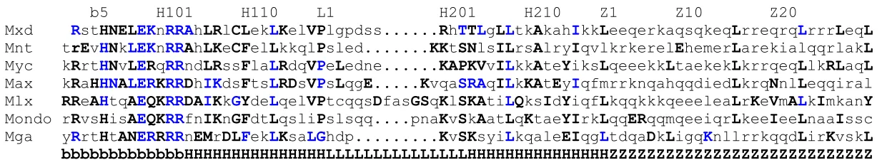
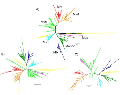
in nematodes formed a Mxd-like (MDL-1), a Myc and Mondo-like (MML-1), a Mlx-like (Mxl-2), and two Max-like (Mxl-1, Mxl-2) proteins. Phylogenetic reconstruction of the bHHZ domain shows distinct conservation among orthologous proteins, while multivariate discriminant analysis reveals particular residues that classify proteins, families, and network configurations. Such differences likely affect the recognition of gene target sequences, and hence alter the function of these transcription factors.

(3)

Modeling the Molecular Evolution of Protein Domains and Networks

by

Lisa Gail McFerrin

A dissertation submitted to the Graduate Faculty of North Carolina State University

in partial fulfillment of the requirements for the Degree of

Doctor of Philosophy

Bioinformatics

Raleigh, North Carolina

2010

APPROVED BY:

_______________________ _______________________

Eric Stone William Atchley

Co-chair Co-chair

_______________________ _______________________

(4)

Dedication

To my family and friends. Without you, nothing would be possible.

Rachel and Ashley, you have been there for me even when you didn’t know it. Thank you for being my rock and keeping me optimistically honest.

My Hokies, you are my spirit. Thank you for keeping my passion for life strong and never letting me take myself too seriously.

My friends both new and old, you always know how to make me smile. Thank you for filling my memories with laughter.

My family, you continually give me strength. Thank you for teaching and encouraging me to be the best I can be.

(5)

Biography

(6)

Acknowledgements

Thank you to my advisors Bill Atchley and Eric Stone. You have been there for me as both friend and mentor. I will never forget our trips to New York, China, and Applebees. I couldn’t have asked for better people to share in this learning endeavor.

Thank you to my committee members Jeff Thorne, Spencer Muse, and Ignazio Carbone for your time, comments, and contribution.

Thank you to the faculty and staff of the Bioinformatics Program and Department of Genetics at the North Carolina State University for your friendliness and unabated willingness to help.

(7)

List of Tables!

Chapter 2: The Non-Random Clustering of Non-Synonymous Substitutions and its Relationship to Evolutionary Rate

Table 1. Genome-wide relationships between log(!) and log(") for eight pairwise

comparisons ... 66!

Table 2. Correlation and partial correlation between log(!) and various protein attributes... 67

Chapter 3: Evolution of the Max and Mlx Networks in Animals Table 1. Max and Mlx Network Members ... 108

Table 2. Sampled Genomes ... 109

Table 3: Phylogenetic Reconstructions ... 110!

Table 4: Discriminant Analysis of Max and Mlx Network Proteins ... 111!

Chapter 4: A Bioinformatics approach towards annotating the glucose response of MondoA and ChREBP Table 1: Proline and Glutamine Rich Region... 162!

(11)

List of Figures!

Chapter 1: Introduction and Background

Figure 1: Probabilistic Models of Evolution ... 6!

Figure 2: Known Max and Mlx Network Configurations ... 15!

Figure 3: Myc:Max and Mxd:Max bHLHZ Structures ... 16!

Figure 4: Max and Mlx Network Member Domains ... 18!

Chapter 2: The Non-Random Clustering of Non-Synonymous Substitutions and its Relationship to Evolutionary Rate Figure 1: Illustration of simple de novo annotation... 62!

Figure 2: Construction of the Dispersion Ratio... 63!

Figure 3: Phylogeny of the eight species considered in pairwise comparisons... 63!

Figure 4: Relationship between measures of selection and dispersion... 64!

Figure 5: Deviation of genes under recent positive selection in humans ... 65!

Chapter 3: Evolution of the Max and Mlx Networks in Animals Figure 1: Max and Mlx Network Protein Distribution ... 101!

Figure 2: Mxd, Myc and Mondo Synteny ... 102!

Figure 3: bHHZ Entropy for Max and Mlx Network members... 103!

Figure 4: HMMER Sequence of bHLHZ domain ... 104!

Figure 5: Phylogeny of bHHZ domain ... 105!

Figure 6: bHHZ PhyML Rooted Tree ... 106!

Figure 7: Nematode bHLHZ Structure ... 107!

Chapter 4: A Bioinformatics approach towards annotating the glucose response of MondoA and ChREBP Figure 1: Phosphorylation Model depicting ChREBP response to glucose ... 152!

Figure 2: Mondo Sequence and Structure Conservation ... 153!

Figure 3: Mondo Conserved Regions ... 154!

Figure 4: Nuclear Receptor Box Conservation... 155

Figure 5: MCRII Helical Wheel ... 155!

Figure 6: Mondo and Mlx DCD Alignment ... 156!

Figure 7: DCD/WMC Entropy ... 157!

Figure 8: DCD/WMC Structure... 158!

Figure 9: G6P Binding Region ... 159!

Figure 10: MondoA N-terminus structure ... 160!

(12)

Appendix A: Statistical Methods for analyzing High Dimensional Molecular Data (HDMD)

(13)

Forward

(14)

Chapter 1 Introduction and Background

A protein is a linear chain of amino acids connected by peptide bonds that can fold into a three-dimensional tertiary structure. Amino acid physicochemical properties such as hydrophobicity, polarity, volume, Van der Waals forces, and hydrogen bonds confer physicochemical constraints that affect protein structure and function (Kidera, Konishi et al. 2009). Often amino acids with similar, overlapping traits can function interchangeably within the protein context, e.g. leucine to isoleucine, while other replacements would likely abrogate protein function, e.g. leucine to proline (Majewski and Ott 2003). One method of inferring the extent of these constraints is to compare orthologous proteins that originate from a common ancestor yet retain similar functions in independently evolving species. Sites with particular amino acid restrictions are expected to be conserved over large evolutionary times while sites exhibiting variability are likely to indicate random or adaptive changes. In general, buried residues and active sites are highly conserved while surface residues are more variable in a folded protein (Ma, Elkayam et al. 2003; Tuncbag, Gursoy et al. 2009). Herein we focus on the development and application of methods to accurately quantify and distinguish factors constraining protein variation in the pursuit of understanding protein function and evolution.

Multiple Sequence Alignments

According to the NCBI website, 564 Eukaryotic and 1956 Prokaryotic genomes have been or are being sequenced as of October 2010 (Sayers, Barrett et al. 2010). One can query such a genome database to find significantly conserved sequences from several diverse species and infer their evolutionary relationship or functional similarities.

(15)

Gumbel Extreme Value Distribution, which depends on the query sequence length, database sequence length, substitution matrix, gap penalties, sequence composition, and the number of sequences in the database. The expected value (E-value) of a particular BLAST alignment score S is the expected number of sequences that would score at least as high as S by chance within the database. Alignments with extremely low E-values may indicate a common function or origin between sequences, although it is important to note that similarity does not necessarily imply homology. Since many genomes are not fully annotated, these genomic resources are useful for identifying and annotating potential orthologs in diverse organisms and supplying a comprehensive sample for comparative analysis.

Analyses of sequence evolution rely heavily upon adequate sampling of sequence variability as well as quality of the sequence alignment. Correct alignment is crucial for testing the magnitude and direction of evolutionary pressure on a site. Unfortunately, aligning multiple orthologous sequences is not a trivial task (Carrillo and Lipman 1988; Wang and Jiang 1994). Dynamic programming methods like the Needleman-Wunsch global alignment and Smith-Waterman local alignment algorithms provide optimal solutions, but require too much computational time and memory to be feasible for many sequences (Feng and Doolittle 1987; Taylor 1988; Lipman, Altschul et al. 1989; Elias 2006; Kumar and Filipski 2007). Ultimately, the trade-off in alignment algorithms is speed versus accuracy, with the former generally prevailing. Hence visual inspection of the aligned sequences is necessary to ensure alignment columns accurately represent homologous sites.

(16)

errors and to sequences of different lengths (Fitch and Smith 1983; Thompson, Plewniak et al. 1999; Pollard, Bergman et al. 2004; Kumar and Filipski 2007).

The global Muscle (Edgar 2004) and local Dialign (Subramanian, Kaufmann et al. 2008) iterative methods avoid initial alignment traps by realigning subsets of sequences and show mild improvements for some alignments. Other methods include the likelihood and optimization algorithms used in Hidden Markov Models (HMMs), simulated annealing, and genetic algorithms, although they are used less commonly due to setbacks in speed and parameter requirements (Kim and Pramanik 1994; Notredame and Higgins 1996; Lassmann and Sonnhammer 2005; Song, Liu et al. 2010). Mafft, which uses a fast Fourier transform to identify homologous regions, has been shown to outperform most of these methods in both speed and accuracy (Katoh, Misawa et al. 2002).

A good operational scheme for attaining accurate alignments is to use an algorithm such as Altavist (Morgenstern, Goel et al. 2003), which computes both a local (Dialign) and global alignment on the data and allows for alignment comparison. Regions where the two algorithms agree are accepted as "correct", while regions where the two algorithms differ can be manually adjusted. Once an alignment is established, evolutionary constraints can be inferred through several methods including selection, phylogenetic and covariance models.

Models of Selection

Protein constraint is the limitation in (physicochemical, structural, binding, etc.) properties a functional polypeptide can tolerate within a certain environment. From sequence alignments, protein constraint can be observed by the non-stochastic pattern of changes in nucleotides, codons, or amino acids.

(17)

especially for large populations (Fisher 1930). A more recent theory of “near neutrality” looks for a balance between these concepts and considers the interaction and importance of drift and selection at various levels, e.g. silent and amino acid altering substitutions and sequence turnover of regulatory elements (Ohta 2002). Consequently, the lack of a definitive evolutionary model lead many to agree with the well-known statistician George Box, “All models are wrong, but some are useful” (E. P. Box and Richard Draper 1987).

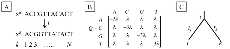
Still, models of evolution can determine the relative intensity and direction of selection among orthologous proteins by comparing the number and type of observed changes. The expected number of changes per site, or evolutionary distance, between orthologs provides a measure of sequence conservation via a specified model of substitution (Jukes and Cantor 1969; Tavaré 1986). Let qij be the instantaneous rate of a site changing from state i to j and Q be the matrix of all possible transitions between states. For DNA models, states consist of the four nucleotides, i, j ={A, C, G, T}, while protein models have 20 amino acid states and codon models have 61 states of nucleotide triplets (excluding stop codons). To retain the probabilistic framework, each site is required to be within a defined state and each row of Q must sum to zero. The probability a site in state i will change to state

j after time t is defined as

!

P(t)=eQt. Assuming site independence in a pairwise sequence comparison, the likelihood of observing the alignment of sites k=1...N is thus

!

L= "_x kaP xk

d _|_x k a_,Qt

(

)

k

#

where ! represents the state stationary frequency for ancestral

sequence xa and descendant sequence xd separated by time t (Figure 1a). The goal is to optimize the estimated substitution rate parameters associated with Q that maximize the probability of observed data.

Note that rate and time cannot be disentangled, but must be jointly estimated. The expected number of changes between sequences after time t is empirically estimated as

distance

!

ˆ

d =t "_jq ˆ _ij i#j

$

where substitution rate

!

ˆ

q _ij_{is estimated from the data. This distance}

(18)

The simplest model of sequence evolution is the Jukes Cantor (JC69) model of nucleotide substitution (Jukes and Cantor 1969). The JC69 model assumes every nucleotide changes at the same rate ", so qij =! when i"j and qij=-3! otherwise (Figure 1b). Thus, after

time t, a site has probability

!

p_r(t)=1_{4 1}

(

+3e"4d 3

)

of remaining in the same state and

probability

!

p_r(t)=1₄

(

1"e"4d 3

)

of being in a different state where distance d=3!t. The

estimated distance between two aligned sequences is then

!

ˆ

d ="3_{4 ln 1}

₍

"4 ˆ p 3

₎

_{, where}

!

ˆ p is the

observed proportion of nucleotide changes. Other increasingly complex models account for different substitution rates among transitions and transversions (Kimura 1980), unequal base compositions (Felsenstein 1981; Tamura and Nei 1993), and combinations thereof (Hasegawa, Kishino et al. 1985).

Figure 1: Probabilistic Models of Evolution

A) Ancestral and Descendant Sequences. The likelihood of observing an alignment of ancestral xa_{and descendant x}d_{sequences separated by time t depends on the probability of states for each} of the N sites. B) JC69 Substitution Matrix Q. C) A Simple Tree. Ancestral sequences are inferred at node i using descendant sequences at children nodes j and k connected by branch lengths tj and tk, respectively.

Codon models further incorporate the effects of non-synonymous (amino acid altering) and synonymous (silent) changes on protein structure and function. The non-synonymous/synonymous substitution rate ratio (!) is predominantly used to assess the

selective pressure for a protein, where !>1 and !<1 indicate diversifying (positive) and

purifying (negative) selection, respectively. A neutral rate of codon evolution occurs when non-synonymous changes accumulate at an equal rate as synonymous changes, or !=1.

Methods using counting techniques estimate ! for individual sites and optionally incorporate

variation in the transition/transversion ratio (Li, Wu et al. 1985; Nei and Gojobori 1986;

! Q= A C G T

A C G T

"3# # # # # "3# # # # # "3# # # # # "3# $ % & & & & ' ( ) ) ) ) i k j t_k t_j

xa_ACCGTTACACT

xd_ACGGTTATACT

t

k= 1 2 3 ….. N

(19)

methods conservatively estimate ! by assuming site independence and averaging ! over the

entire sequence. Alternatively, sophisticated likelihood methods can be coupled with probabilistic models of phylogenetic relationships to incorporate the evolutionary history of a protein. Numerous codon models exist with variable specifications on substitution rates, including MG94 (Muse and Gaut 1994) and GY94 (Goldman and Yang 1994), which allow for position specific nucleotide substitution rates within the codon.

Several recent studies have found that the synonymous substitution rate is not neutral and can be influenced by factors such as exonic splicing enhancers, codon usage bias, isochores, translational rate or mRNA structure (reviewed in Chamary, Parmley et al. 2006). Kosakovsky Pond and Muse (2005) found that allowing separate non-synonymous and synonymous rates for each site more accurately represented their datasets 9 of 10 times. In a similar manner, Mayrose et al. (2007) allow for separate non-synonymous and synonymous rates and propose the instantaneous rate of changing from codon i to codon j be defined by:

!

Q_ij =

"_s#$#% _j iand j differ by one synonymous transition "s#% j iand j differ by one synonymous transversion "_a #$#% _j iand j differ by one non&synonymous transition "a #% j iand j differ by one non&synonymous transversion

0 otherwise

'

( ) ) )

* ) ) )

where !j is the target codon frequency calculated using the F3x4 model (Yang, Nielsen et al.

2000), " is the transition/transversion ratio, and #s and #a are the synonymous and

non-synonymous substitution rates. Substitution rate parameters can be optimized to maximize the likelihood of observed data and estimate the evolutionary distance between sequences.

Models can also allow for heterogeneous substitution rates among sites, which can be estimated from given a distribution, e.g. Poisson, Beta, Normal, or Gamma. While rate heterogeneity approximates a more biologically realistic model (Yang, Nielsen et al. 2000), it is computationally intensive and often requires discretization of a continuous distribution. Due to the pliability of the gamma distribution based on the shape ($ >0) and scale (% >0)

(20)

the likelihood. To circumvent this issue, a discrete gamma model can be approximated by K

rate categories, each weighted by their probability of occurrence and represented by substitution rate rk, a summary statistic for rate category k (Yang 1994; Stern and Pupko 2006). When $ < 1 the gamma distribution becomes skewed and has an L-shape, $ & 1

creates a '-shape, while $() reduces the model to a single rate across all sites. By

estimating parameters $ and %, the mean $/% and variance $/%2 of the gamma distribution

can be used to describe the distribution of synonymous #s and non-synonymous #a

substitution rates. For example, when

!

ˆ

"_s=#ˆ _s the synonymous substitution rate

!

"_s~#( ˆ $_s, ˆ $_s)

will be neutrally evolving with mean 1 and variance

!

1 ˆ " _s while a non-synonymous

substitution rate

!

"_a ~#( ˆ $_a, ˆ %_a) will have a variable level of selection (Mayrose, Doron-Faigenboim et al. 2007). After maximizing the likelihood, rigorous statistical methods can test for significant trends in selection by comparing the estimated non-synonymous and synonymous substitution rates.

For large evolutionary distances, the use of nucleotide or codon sequence alignments may not be appropriate due to the possible saturation of substitutions. Instead heuristic amino acid models better reflect the probability of changes affecting protein structure and function (Halpern and Bruno 1998). Originally Dayhoff et al. empirically estimated the substitution rates among amino acids using observed changes in an alignment of orthologous proteins with at least 85% identity (Dayhoff, Schwartz et al. 1978). The symmetric 20x20 matrix was then standardized to create PAM1, which has one accepted point mutation per 100 amino acids. Assuming changes occur independently, repeatedly multiplying PAM1 creates matrices that reflect more divergent sequences such as PAM250 with an average of 2.5 changes per residue. Since only a few protein families were available during the initial calculation, a similar method has since been reapplied to create the updated JTT matrix based on a large set of protein databases (Jones, Taylor et al. 1992).

(21)

log-odds scores comparing the log ratio of likelihoods for residues in a biological alignment against those paired by random chance. The BLOSUM80 matrix was calculated by comparing sequences with at least 80% identity while BLOSUM45 used sequences with at least 45% identity. Hence lower valued BLOSUM matrices are more appropriate for estimating relationships for more divergent sequences.

Phylogenetics

The rate of sequence evolution varies extensively among genes and DNA segments. Representing the estimated evolutionary relationships of homologous sequences in a phylogenetic tree provides a useful tool for visualizing the patterns and processes of evolution (Felsenstein 1981). For example, cladogenesis can indicate speciation or duplication events, while branch lengths can signify the extent of divergence. However, a matrix of pairwise distance estimates does not necessarily form an exact or unique bifurcating tree due to violations of the triangle inequality (Beyer, Stein et al. 1974) and inaccuracies arising from the summarization of the phylogenetic information into a single distinct value. Exhaustively comparing all possible trees is infeasible since an alignment of

just m=10 sequences will have

!

2m"3

( )!!=₍2m"3₎! 2m"2₍m"2₎!=34,459,425 possible bifurcating,

rooted trees (Felsenstein 1978). Stepwise algorithms and heuristic search methods are often applied to reduce computational cost at the expense of rigor. Hence determining proper tree reconstruction and inference methods is not straightforward because of the statistical and biological assumptions used to circumvent these issues.

(22)

uses total tree length as the criterion for tree selection, and may poorly estimate large distances or trees based on alignments containing numerous gaps. A related method called BIONJ addresses this shortcoming in NJ trees by incorporating the approximate variance and covariance of distance estimates (Gascuel 1997). Likewise, WEIGHNJ uses an approximate likelihood criterion for joining nodes to make the method more robust and produce trees similar to the maximum likelihood method described below (Bruno, Socci et al. 2000).

Parsimony, Maximum Likelihood (ML) and Bayesian methods are all character based tree estimation procedures. These methods search the tree space using an objective function, fit each observed character (nucleotide, codon, or amino acid) at every site to a tree, and measure the fit of data to that tree. This procedure is very laborious and time consuming for a large number of sequences, as each iteration through the tree space requires a measure of fit calculation (Felsenstein 2004). Nonetheless, rich, statistical theory has been established to allow for comparison of estimates and likelihoods among trees.

ML and Bayesian methods easily incorporate complex models with realistic biological assumptions to provide a powerful and flexible framework for phylogenetic inference and hypothesis testing. The ML method fits data from a given alignment (D) to a tree topology (T) using a particular model of evolution by maximizing the likelihood function L=P(D|",T), where " is the set of model parameters to be estimated. These parameters

include the frequency of character states, branch lengths, substitution rates, and rate heterogeneity among sites (Durbin, Eddy et al. 1998). Assuming a general time reversible model where the rate of substitution from state xi to xj is the same as xj to xi and

!

"_iQ_ij="_jQ_ji, we can apply Felsenstein's pruning algorithm to quickly calculate the likelihood at each site (Felsenstein 1981). For node i with children nodes j and k connected by branch lengths tj and

tk respectively (Figure 1c), define

!

Li( )xi = px_ix_j(tj)Lj(xj) " xj

#

px_ix_k(tk)Lk(xk) xk

#

as the

probability of observing the data at node i and its descendants, given its character is in state

xi. The total likelihood for site s is then L(s)= "xiL0(xi) xi

#

where L0 is the likelihood at the root

(23)

likelihood of the tree is simply the product of site likelihoods. Since this value is typically small and difficult to store computationally, the log likelihood is calculated instead where

!

!=log(L)= log

s

"

( )

L(s) _{. A deficiency with the ML algorithm is that the common and}

biologically more realistic case of intercorrelated or dependent sites complicates the likelihood model (Yang 1995; Felsenstein and Churchill 1996; Mayrose, Doron-Faigenboim et al. 2007; Fernandes and Atchley 2008). This condition exponentially increases the size for substitution matrix Q and is rarely implemented due to the extremely cumbersome computation.

The Bayesian method of phylogenetic reconstruction similarly uses an explicit model of evolution to optimize a likelihood function. This procedure optimizes the posterior probability P("|D) using Bayes Theorem,

!

P₍" |D₎=P D( |")P( )" _{P D}

( )=

P D₍ |"₎P_{( )}"

P(D|")P(")d"

#

where T is incorporated in the set of model parameters ", D is as described above, P(D|") is

the likelihood, P(D) is the marginal probability of the data given a tree, and P(") is the prior

distribution describing the tree parameters. A prior distribution allows for the incorporation of additional biological information during estimation and defines a confidence interval for the model parameters rather than a point estimate as in ML. When no information is available a priori, a noninformative prior is assumed and a uniform distribution is used. Arguably, a uniform distribution does not imply an uninformed prior and there is significant disagreement over the use and interpretation of prior distributions (Syversveen 1998). To complicate matters further, the marginal probability of the data in the denominator is difficult if not impossible to calculate. The Markov Chain Monte Carlo (MCMC) algorithm circumvents this issue by optimizing the posterior distribution (Metropolis, Rosenbluth et al. 1953; Hastings 1970).

In a non-periodic Markov Chain, each state represents a set of " values with a

stationary distribution of P(_"|D), assuming each state can reach any other state within a finite

(24)

large number of " values from P("|D) under the expectation that " values with a high

posterior probability are more likely to be sampled than those with a low posterior probability. Thus running the Markov Chain for a sufficient period of time can approximate

P("|D) by the probability of being at a particular state. Starting at time t=0 with parameter

values "(t),the algorithm steps through the Markov Chain and randomly proposes a new set

of parameter values "*. The Hastings algorithm accepts these new "* values with probability

min(1, r), where

!

r=P(D|"

*₎_P₍_"*₎_J₍_"(t)_|_"*₎

P(D|")P(")J("*|"(t)) and

!

J("(t)|"*) is the probability of "jumping"

from "(t)to "* (Hastings 1970). Current limitations to the MCMC Bayesian method arise

from difficulties in assessing independence from initial parameter specifications, correlations in consecutive parameter values, and ensuring the process does not get trapped in local maxima. In spite of these difficulties, the MCMC Bayesian method provides a straightforward interpretation of probabilities and easily lends itself to biological models (Marjoram and Tavaré 2006).

Likelihoods produced by Bayesian and ML methods quantify the fit of data for a given tree and model of evolution. Statistical methods can then compare multiple likelihoods

to identify the model of better fit. The likelihood ratio statistic,

!

LRT="2 L1

L₂ # $

% &

'

(, compares

likelihoods for two nested models to test if the likelihood of a model with more parameters, L2, is significantly better than that with one or more fixed parameters, L1 (Casella and Berger 2002). The Chi-squared distribution can then be used with df1-df2 degrees of freedom to compare the fit of models. However, by definition L2 # L1 and the increase in parameters may cause overfitting. The Akaike information criterion (AIC) and Bayes information criterion (BIC) measure the goodness of fit for model selection while penalizing overparameterization (Akaike 1974; Schwarz 1978). Lower AIC or BIC values indicate the preferred model. In general,

!

AIC=2k"2 ln(L) with k estimated parameters and maximized likelihood L for the given model. BIC imposes a stricter penalty than AIC for including

additional parameters and is defined by BIC="2 ln

₍

p(x|k)

₎

="2 ln(L)+kln(n), where data x

(25)

Bayes, MEGA, Phylip, PhyML, BioNJ, Weighbor) for constructing and testing phylogenies is available in Chapter 3.

High Dimensional Molecular Data

Some methods of identifying selection focus on statistically quantifying protein property variability. Many such tests require extensive replication for sufficient power to determine significance, and most exploratory techniques like genome sequencing and microarrays inundate biologists with massive amounts of high dimensional molecular data (HDMD). These huge data sets lead to major statistical issues since HDMD typically have many more variables than observations. This condition, often called "the curse of dimensionality" (Bellman 1961), causes various multivariate statistical analyses to fail, become intractable, or produce misleading results (Donoho 2000; Ransohoff 2005; Clarke, Ressom et al. 2008). Further, there are serious problems with procedures used to effectively reduce the dimensionality of HDMD while retaining relevant biological information. Widely used multivariate techniques like cluster analysis (MacQueen 1966; Overbeek, Fonstein et al. 1999; Tan, Steinbach et al. 2006), principal component analysis (PCA) (Jolliffe 2002; Johnson and Wichern 2007), factor analysis (FA) (L. Gorsuch 1983), and discriminant analysis (DA) (J. Huberty 1994) have underlying assumptions that are often not properly addressed.

In Chapter 3 we employ FA and DA to identify variability due to selection in the DNA binding and dimerization domain of Max and Mlx proteins. While that chapter includes a brief summary and purpose in using these methods, we provide Appendix A to further discuss a number of problems pertaining to HDMD and the relative merits of these and various multivariate statistical procedures.

Max and Mlx Networks

(26)

The Max network of interacting transcription factors regulates cell cycle progression via coordinated activation or repression of genes involved in ribosome biogenesis, growth, proliferation, differentiation, and apoptosis (reviewed in Lüscher 2001). Antagonistic dimerization of Myc and Mxd/Mnt to obligate partner Max governs transcriptional activation and cell proliferation or transcriptional repression and cell differentiation, respectively. Similarly, repressors Mxd/Mnt and transcriptional activator Mondo competitively and antagonistically dimerize with Max-like protein Mlx in the parallel Mlx network, which is implicated in cellular proliferation, growth, energy homeostasis, and metabolism (Billin and Ayer 2006).

Implications in Disease

Deregulation of the Max and Mlx networks leads to improper cell growth, unbalanced energy homeostasis, and possibly death (Lüscher 2001; Billin and Ayer 2006). Myc family member c-Myc has long been known as a potent proto-oncogene that is necessary for cell growth in mammals, yet often deregulated in actively growing tumors (Eilers and Eisenman 2008). Although not properly identified as a tumor suppressor protein, Mnt antagonizes c-Myc function and can also promote tumor growth when conditionally deleted (Hooker and Hurlin 2006). Since Mnt, c-Myc and Max have complex function and are essential for mammalian viability, using them as drug targets in cancer treatments has proved challenging (Freie and Eisenman 2008). Similarly, MondoB is implicated in cell growth and particularly in glucose metabolism (Yamashita, Takenoshita et al. 2001). As a major factor in de novo

(27)

Known Max and Mlx Network Configurations

Less complex organisms can often act as adequate surrogates for annotating proteins as well as protein networks. To date, three main Max and Mlx network configurations have been documented in vertebrates, flies, and nematodes (Figure 2).

Figure 2: Known Max and Mlx Network Configurations

A) Drosophila melanogaster, B) Caenorhabditis elegans, C) Mus musculus. Red trapezoids represent repressor proteins, green rectangles activating proteins, and blue ovals central interaction partners. Solid lines indicate known bHLHZ interactions, while dotted lines have not been firmly established.

The vertebrate network has paralogous families for Myc (c-, L-, and N-Myc), Mxd (Mxd1-4, formerly Mad1, Mxi1, Mad3, and Mad4) and Mondo (MondoA and MondoB), along with single copies of Max, Mlx, Mnt, and Mga genes. In addition, rodents have experienced lineage specific duplications to create S-Myc and b-Myc, while the human network contains a separate duplication denoted L-Myc2 (Lüscher 2001). For the purposes of this discussion, b-Myc in rodents is not included within the Max network since it lacks a bHLHZ domain (Burton, Mattila et al. 2006). Mediated by the highly conserved bHLHZ domain, Max can homodimerize with itself and heterodimerize with Mnt, Mga, and members of the Myc and Mxd families (Hurlin and Huang 2006). The Mlx bHLHZ domain exhibits a more restrictive binding pattern and interacts with only Mxd1 and Mxd4 of the Mxd family in addition to itself, MondoA, and MondoB (Billin and Ayer 2006).

Drosophila melanogaster contains a simpler network with single genes coding for dMyc, dMax, dMlx, dMnt, and dMondo (Gallant 2006). Vertebrate c-Myc is considered a direct ortholog of dMyc due to their similar cellular expression and reciprocal ability to rescue dMyc-/- Drosophila mutants and c-Myc null murine embryo fibroblasts (MEFs) (Gallant, Shiio et al. 1996; Delacova and Johnston 2006). As before, dMax can dimerize

MLX MAX MONDO MYC MNT MXL1 MML1 MDL-1 MXL2

MXL3 MLX MAX MONDOB cMYC MXD1 MXD4 MONDOA NMYC LMYC MXD2 MXD3 MNT

MGA _SMYC

A

B

(28)

with dMax, dMyc and dMnt, while dMlx binds to dMondo. Interestingly, the loss of Mxd in flies makes dMnt the only repressor within this network.

Caenorhabditis elegans has a markedly different yet clearly orthologous network, presumably due to massive gene reduction and rearrangement in nematodes (Witherspoon and Robertson 2003; Denver, Morris et al. 2004; Coghlan 2005). Notably, C. elegans lacks both Mnt and Myc orthologs. Instead, Myc and Mondo-like protein MML-1 and Mad-like ortholog MDL-1 alone comprise the activator and repressor components of the network, respectively, while two Max orthologs (Mxl-1 and Mxl-3) and a single Mlx ortholog (Mxl-2) act as central dimerization partners (Yuan, Tirabassi et al. 1998). Mxl-2 dimerizes to transcriptional activator MML-1, while MDL-1 dimerizes with either Mxl-1 or Mxl-3 to repress transcription. Surprisingly, Mxl-1 cannot homodimerize and does not interact with mouse c-Myc.

As the defining factor for Max and Mlx network members, the bHLHZ domain is integral for their protein-protein and protein-DNA interactions (Nair and Burley 2006; Maerkl and Quake 2009). Dimerization of obligate partners through the bHLHZ domain creates a four helix amphipathic bundle for which several structures have been determined and are available in the protein databank (PDB): Max:Max heterodimer (1R05), Max:Max heterodimer recognizing DNA (1AN2, 1HLO), Max:Mxd1 heterodimer recognizing DNA (1NLW), Max:Myc heterodimer/heterotetramer recognizing DNA (1NKP), and Max:c-Myc leucine zipper (1A93, 2A93) (Ferré-D'Amaré, Prendergast et al. 1993; Brownlie, Ceska et al. 1997; Lavigne, Crump et al. 1998; Nair and Burley 2003; Sauvé, Tremblay et al. 2004).

Figure 3: Myc:Max and Mxd:Max bHLHZ Structures

(29)

Max network proteins are known to bind to the E-box motif 5’-CACGTG-3’ (Blackwood and Eisenman 1991; Blackwell, Huang et al. 1993), while MondoA, MondoB, and Mlx bind a ChORE motif characterized by two E-boxes separated by exactly five nucleotides, CAYGNGN5CNCRTG (Ma, Robinson et al. 2006). Due to the importance of the bHLHZ domain in these essential and potentially proto-oncogenic proteins, we examined the sequence conservation and functional characteristics of the bHLHZ domain among network members, and present our results in Chapter 3.

Sequence variability in regions surrounding the conserved bHLHZ domain and presence of other functionally disparate domains suggests these proteins arose through ancient domain shuffling events, Figure 4 (Morgenstern and Atchley 1999; Jones 2004). The N-terminus of activators Myc, Mondo, and MML-1 contain a transactivation domain (TAD), while repressors Mnt, Mxd, and MDL-1 have a Sin3 interaction domain (SID) (Lüscher 2001; Hurlin and Huang 2006). Myc's TAD associates with coactivator complex TRRAP/GCN5 and the subsequent Myc/Max/TRRAP/GCN5 active complex binds to the DNA E-box motif, acetylates surrounding histones, and permits transcriptional activation of gene targets. In contrast, Mnt, Mxd, and MDL-1 recruit the Sin3/HDAC/N-Cor/Ski/Sno complex to its SID, which in turn deacetylates histones and represses transcription. Max and Mlx lack any other known functional domain and therefore simply serve as necessary coactivators.

(30)

Figure 4: Max and Mlx Network Member Domains

Modified from (Lüscher 2001). TAD: transactivation domain, bHLHZ: basic-Helix-Loop-Helix-Leucine Zipper domain, Transrepression Domain: region involved in repression, SID: mSin3-interaction domain, T-Domain: T-box DNA binding domain, DCD: dimerization and cytoplasmic localization domain.

Myc and Mxd affect Cell Cycle Progression

The cell cycle is responsible for cell duplication and division and is defined by the resting phase (G0), two gap or growth phases (G1, G2), a DNA synthesis phase (S), and mitosis (M). Quiescent or differentiated cells are in resting (G0) phase of the cell cycle, while proliferating cells cycle through G1, S, G2, and M.

In normal cells, mitogen-induced expression by c-Myc is sufficient to initiate cell cycle entry in otherwise quiescent or differentiated cells endogenously expressing Mxd1, Mxd2, and Mxd4 (Eilers, Schirm et al. 1991; Walker, Zhou et al. 2005). c-Myc accumulates quickly during G1 phase and displaces Mnt as the primary Max dimer to activate key mitosis checkpoint proteins like cdk4, CycD, CycE, and Rbf (Hooker and Hurlin 2006). Ubiquitin-mediated proteolysis degrades existing c-Myc rapidly, while a negative feedback loop prevents further protein production. This subsequent degradation of c-Myc is important to protect against tumorigenesis and increased sensitivity to apoptosis as high levels of c-Myc during S phase are linked to an increased susceptibility to mutation (Felsher and Bishop

(31)

1999). c-Myc levels return to a low, steady state by S phase, whereby Mxd3 accumulates, peaks and diminishes again.

The coordinated oscillation of c-Myc and Mxd expression during cell cycle transitions of proliferative/quiescent states and G1/S phases suggests these proteins act as an on/off switch governing transcriptional activation or repression of genes specific to cell cycle progression. Such transitioning between Max heterodimerization partners depends on the relative expression levels, complex stability, subcellular location, and protein degradation of Myc, Mxd, and Mnt proteins. Max levels are in excess compared to its binding partners and competition may only occur during peak phases of expression for its interacting proteins (Lüscher 2001).

The following addresses the individual and coordinated functions for Max network components, with regard to their role in cell cycle regulation and transformation.

Max is a central dimerization partner

Max is a small essential protein with ubiquitous and cell autonomous expression and is maintained at constant, stable levels with a half-life of >24hours (Blackwood et al, 1992). An 'RKKLR' motif located near the bHLHZ domain serves as a nuclear localization signal (NLS) that transports Max to the nucleoplasm where it is uniformly distributed (Grinberg, Hu et al. 2004). In the absence of other interacting proteins, Max readily forms Max:Max homodimers that bind to E-box motifs and weakly decrease transcription by $2-fold (Billin, Eilers et al. 1999; Mcduff, Naud et al. 2009). The function of DNA-bound Max:Max is unknown, since Max has no discernable phenotype and contains no other known domain. Instead Max may mark genes poised for transcriptional regulation, possibly binding to DNA as a monomer prior to dimerization. As such, Max function depends on the conditional expression, cellular location, and relative binding affinity of the Myc, Mnt, Mxd, and Mga interacting proteins described below.

Myc is a potent proto-oncogene

(32)

Myc abundance is tightly regulated due to its essential role in growth and is typically expressed only at low levels in proliferating cells (Hooker and Hurlin 2006). That said, Myc deregulation is associated with most if not all cancers, attributing to around 70,000 deaths a year (myccancergene.org). Translocation and amplification, activation of growth signals, and increased protein stability contribute to its deregulation (Spencer and Groudine 1991). The transformation behavior stems from Myc's ability to induce proliferation through cell cycle entry, block cell cycle exit, and sensitize cells to apoptosis in a manner dependent upon cell type and physiological status (Grandori, Cowley et al. 2000; Nasi, Ciarapica et al. 2001). Although aberrant overexpression of Myc does not accelerate cell division, it can prevent cell cycle exit with a correspondingly marked increase in cell and consequently body size (Johnston, Prober et al. 1999).

In a normal cell, overabundance of Myc triggers a Myc induced apoptotic pathway in both a p53-dependent and -independent fashion as a failsafe mechanism to limit excessive growth and control tumor progression (Hoffman and Liebermann 2008). Frequently, cells with overexpressed Myc have mutations that disrupt this pathway, allowing survival, exacerbating proliferation, and further promoting transformation (Grandori, Cowley et al. 2000; Hooker and Hurlin 2006). Ectopic upregulation of Myc can also disrupt normal cell function and result in tumor formation, e.g. just a 1.47 fold increase of c-Myc was observed in certain cases of Burkitt's Lymphoma (Sáez, Artiga et al. 2003). Moreover, Myc can induce cell competition, where neighboring cells with significantly lower levels of Myc are signaled for apoptosis (Johnston, Prober et al. 1999; Secombe, Pierce et al. 2004). Thus cells experiencing Myc deregulation can increase cell growth and demand for more nutrients, survive longer when the apoptotic pathway is disrupted, and deplete surrounding healthy cells.

(33)

mouse c-Myc-/- mutants arrest development at day 9.5 postcoitum (Davis, Wims et al. 1993), and mice with N-Myc-/- mutants fail to develop heart, lungs, and a nervous system (Charron, Malynn et al. 1992). Curiously, L-Myc-/- mutant mice are viable and lack any major defects (Hatton, Mahon et al. 1996). In comparison, c-Myc hypomorphs have a normal cell size, although the body size is smaller, development is delayed, and females are sterile due to a defect in oogenesis (Gallant, Shiio et al. 1996; Gallant 2006).

Supporting Myc’s role in proliferation, differentiation, and growth, Myc is shown to target genes involved in metabolism (CAD, ornithine decarboxylase, Lactate dehydrogenase A, dihydrofolate reductase), cell cycle progression (cyclinA, cyclinD2, cyclinE, cdc25A, telomerase genes), and ribosome biogenesis (tRNAs and 5S rRNA) (Hooker and Hurlin 2006). However, recent genome scans show Myc can bind globally, spanning ~15% of both the Drosophila and human genome in both inter- and intra-genic regions (Orian, van Steensel et al. 2003). Thus Myc can affect hundreds to thousands of genes, albeit weakly.

To bind DNA and transactivate genes, as well as interact with Inr elements such as Miz-1, Myc must first dimerize with Max (Seoane, Pouponnot et al. 2001; Staller, Peukert et al. 2001; Herold, Wanzel et al. 2002). However, recent evidence in Drosophila indicates Myc can also function in a Max independent manner. Experiments with Drosophila dMax -/-mutants found dMyc can induce biological processes such as cell autonomous death, endoreplication of polyploid larval cells, cell competition, and regulation of cell growth (Steiger, Furrer et al. 2008). Specifically, activation of RNA polymerase II and Myc induced apoptosis, by and large, do not require Max dimerization. Nonetheless, increasing Max expression in response to Myc overexpression can reduce cell transformation, possibly preventing Myc from binding to other interaction partners such as those involved in RNA polymerase formation (Mäkelä, Koskinen et al. 1992).

(34)

Mnt represses cell growth

Myc and Mnt exhibit opposing roles in regulating cell growth, with similar implications in tumor formation when deregulated. Mnt overexpression results in markedly reduced cell and body size, while conditional deletion of Mnt leads to increased cell size, tumor formation, disruption in T cell development, and in general phenocopies c-Myc overexpression (Hurlin, Zhou et al. 2004; Nilsson and Cleveland 2004; Loo, Secombe et al. 2005; Walker, Zhou et al. 2005; Wahlström and Henriksson 2007). However, loss of Mnt function is not equivalent to aberrant Myc expression, since Myc abundance is still under several other regulatory mechanisms (Hooker and Hurlin 2006). Instead, Mnt depletion may increase the expression level and sensitivity of target genes to Myc activation, as seen during cell cycle progression (Walker, Zhou et al. 2005). Correspondingly, tumor formation resulting from conditional Mnt deletion is less penetrant and takes longer than ectopic overexpression of Myc (Hurlin, Zhou et al. 2003). Despite these tumor suppressor properties, cancer cells rarely have mutations in Mnt (Sommer, Waha et al. 1999).

Mnt and Myc’s reciprocal roles in controlling cell growth suggest they share overlapping gene targets. As expected, dMnt and dMyc have both unique and overlapping binding sites (Orian, van Steensel et al. 2003). Since Mnt is ubiquitously expressed in proliferating, quiescent, and differentiating cells, while Myc expression is limited to proliferating cells, Mnt inhibits Myc transactivation as well as suppresses Myc-dependent transformation (Zhou and Hurlin 2001; Hurlin, Zhou et al. 2003). Hence, Mnt can act as a general repressor of Myc to control cell progression, even though Mnt expression is independent of the cell cycle.

(35)

(Walker, Zhou et al. 2005; Hooker and Hurlin 2006). This is in stark contrast to Drosophila

dMyc-/-/dMnt-/- mutants, which grow significantly larger and with increased viability over single mutant dMyc-/- as a result of increased endoreplication and growth of larval tissues and imaginal discs (Pierce, Yost et al. 2008). Since Myc relieves Mnt repression in both mouse and Drosophila models, the discordance of these findings suggests a divergence in network dynamics between species.

As previously mentioned, dMnt is the only repressor in the Drosophila Max network, while Mnt and Mxd1-4 repress Myc family proteins in vertebrates. Also, in contrast to the ubiquitous expression of vertebrate Mnt, dMnt has a dynamic expression pattern temporally dependent upon cell type, where it is present in actively replicating mitotic and endoreplicating tissue as well as differentiating cells (Loo, Secombe et al. 2005). Hence

Drosophila has adopted a distinct balance among Max network members that does not necessarily require Mnt or Mxd proteins. Similarly, C. elegans does not have a Mnt ortholog, but rather contains a Mxd-like ortholog, MDL-1, involved in post-embryonic development and suppression of transformation (Yuan, Tirabassi et al. 1998).

Mxd proteins have dynamic patterns of repression in vertebrates

Like Mnt, Mxd proteins repress Myc and can suppress c-Myc-dependent cell transformation (Lahoz, Xu et al. 1994; Koskinen, Ayer et al. 1995; Västrik, Kaipainen et al. 1995; Zhou and Hurlin 2001). However, the Mxd family of proteins in vertebrates exhibits a dynamic, yet distinct expression pattern that may mediate specialized roles in Myc repression (Hooker and Hurlin 2006).

(36)

expression of Mxd3 peaks during S phase of the cell cycle (Hurlin, Quéva et al. 1995; Quéva, Hurlin et al. 1998; Fox and Wright 2001; Quéva, McArthur et al. 2001).

When bound to Max, Mxd proteins repress transcription of gene targets by $4 fold and mediate cell cycle checkpoints (Billin, Eilers et al. 1999). In particular, Mxd1 represses Myc targets cyclin D2 and human telomerase reverse transcriptase (hTERT), which are important for the transition into and progression of S phase (Günes, Lichtsteiner et al. 2000; Bouchard, Dittrich et al. 2001; Xu, Popov et al. 2001). Mxd3 amplification and c-Myc depletion during S phase further suggests Mxd proteins affect cell cycle progression through phase-specific regulation (Hooker and Hurlin 2006). The reciprocal relationship between Mxd and Myc reflects a switch from activation to repression of gene targets, associated with a transition from cell proliferation to differentiation (Ayer and Eisenman 1993). Due to their short (15-20 minute) half-life, Myc and Mxd families yield a steady turnover rate that enables the network to readily respond to external stimuli and transition between cell states (Blackwood, Lüscher et al. 1992; Amati and Land 1994; Sears 2004; Adhikary and Eilers 2005).

Regulation of cell cycle progression and Mxd mediated antagonism of Myc suggested this family could contain potential tumor suppressor proteins. Accordingly, deletion or Loss of heterozygosity (LOH) in a region containing Mxd2 is associated with tumors including astrocytoma, glioblastoma, lymphocytic leukemia, prostate adenocarcinoma, malignant melanoma, small cell and squamous cell carcinomas of the lung (Edelhoff, Ayer et al. 1994; Chen, Willingham et al. 1995; Eagle, Yin et al. 1995; Foley and Eisenman 1999; Engstrom, Youkilis et al. 2004). However, alterations of Mxd2 were found in only a subpopulation of cells for each tumor and a nearby tumor suppressor gene PTEN/MMAC1 may be responsible (Li, Yen et al. 1997). Similarly, there is no clear indication that Mxd1, Mxd3, or Mxd4 are consistently altered in tumors (Schreiber-Agus and Depinho 1998; Baudino and Cleveland 2001).

(37)

outwardly healthy (Schreiber-Agus and Depinho 1998; Foley and Eisenman 1999; Rottmann and Lüscher 2006). Mxd3-/- mice are healthy, with no apparent defect in cell cycle entry or exit, although thymocytes and neuronal cells are sensitive to radiation-induced apoptosis (Quéva, McArthur et al. 2001). Mxd1-/- and Mxd3-/- mice were also more sensitive to granulocyte differentiation (Foley, McArthur et al. 1998). Surprisingly, simultaneous deletion of Mxd1, Mxd2, and Mxd3 produced mice that were fertile, viable, and 15-20% larger than controls, with a hyperproliferative phenotype in thymocytes, and splenic B and T cells (Rottmann and Lüscher 2006). Since Mxd4 knockouts have not been investigated, it is unknown if Mxd4 is compensating for the triple mutant knockout or if Mxd proteins are dispensable as a whole.

Evidence of protein compensation among Mxd family members suggests a restrictive homeostatic feedback mechanism of upregulation in response to individual gene loss (Rottmann and Lüscher 2006). While other Mxd levels do not change in Mxd2 or Mxd3 knockout mice, Mxd2 and Mxd3 expression is upregulated when Mxd1 is removed (Ayer, Kretzner et al. 1993; Quéva, McArthur et al. 2001). There may also be functional compensation/complementation from proteins outside the Max network, as seen by the synergism between Mxd2 and cki p27 proteins in promoting cell cycle exit during differentiation (McArthur, Foley et al. 2002).

Max and Mlx Networks Overlap

(38)

Immunoprecipitation from cell lysates showed that Mxd1 preferentially dimerizes with Max over Mlx, while two hybrid and gel shift assays using recombinant proteins show similar binding affinities (Billin and Ayer 2006). This indicates post-translational modification moderates the cellular location of these proteins and the preferential binding partner of Mxd1. The preferential binding of Mxd4 to Max or Mlx is unknown.

Mnt has also been found to dimerize with Mlx, but this interaction has not been firmly established. Mnt:Mlx and Mlx:Mlx heterodimers have been isolated (Meroni, Cairo et al. 2000) and Mnt was identified as a Mlx interactor when isolating MondoB:Mlx complexes (Cairo, Merla et al. 2001), yet no further experiments have validated the presence of Mnt:Mlx. In opposition, Mnt:Mlx or Mlx:Mlx interactions were not found (Billin, Eilers et al. 1999) and Mnt:Mlx interaction in vitro or in vivo has not been observed (Hurlin and Huang 2006). Although Mnt:Mlx repression on E-box genes was established (Meroni, Cairo et al. 2000), the level of repression was not significantly different upon addition of Mlx. This suggests the observed repression occurs only under particular cellular conditions and could be mediated by either endogenous Max or Mlx levels or Mlx:Mnt dimerization. Moreover, combinatorial knockouts of Drosophila dMyc (dm4_{), dMnt (Mnt}1_{) and dMax (Max}1_{), show} dm4Mnt1, dm4Max1,and dm4Mnt1Max1 mutants have strong similarity in phenotype (Pierce, Yost et al. 2008). This implies that both dMax and dMnt do not interact with other partners including dMlx or dMondo, at least for the cell type and condition assayed.

Mga function and origin is unknown

(39)

The unusual coupling of multiple DNA binding domains complicates the functional role Mga.

Mga acts as either a repressor or activator of reporter genes in a Max dependent manner (Hurlin, Steingrìmsson et al. 1999). Mga:Max activates transcription when the canonical E-box motif, T-domain, or both are present. Mga:Max*BR also activates

T-domain reporters, where Max*BR is a dominant-negative repressor that lacks the basic

region and cannot bind to the E-box. In the absence of endogenous Max, Mga binds and subsequently represses a T-domain containing reporter. This implies that Mga:Max dimerization through the bHLHZ domain not only permits binding to the E-box motif, but may also block a bHLHZ dependent co-repressor for T-domain targets. Thus Mga acts as a dual specific transcriptional regulator, where activation is dependent upon Max dosage.

From yeast two hybrid assays, Mga was identified in mouse embryonic cDNA libraries at days E9.5 and E10.5 as well as murine kidney cells at E14.5 with highest levels found in limb buds, branchial arches and the tail region (Hurlin, Steingrìmsson et al. 1999). Mga was not isolated in other cell types or adult tissues using Northern blot assay, except in rat pheochromocytoma cell line PC12 and C2C12 myoblasts. The overlapping expression of Mga with other T-box proteins such as Brachyury, Tbx2, 3, 4, and 5 during embryonic development suggests that it also regulates regions involved in mesoderm and mesodermal-epithelial interactions during development. However, little is still known about this large protein including the possible identification of other domains, role of alternative splicing, subcellular location, and cross talk between the bHLHZ and T-box domains.

The Mlx Network

In general, Max network members control cell growth by regulating target genes involved in proliferation, differentiation and cell cycle progression. Similarly, the parallel Mlx network of transcription factors affects cell growth by targeting genes involved in glucose metabolism.

(40)

can be decomposed into glucose and processed through glycolysis and the citric acid cycle (TCA) for energy use. Upon food intake, increased glycolitic flux stimulates insulin secretion from pancreatic islets (%-cells) and activates the glycogen synthesis or de novo lipogenesis pathways in the liver to promote energy storage (Postic, Dentin et al. 2007).

In mammals, MondoB expression in the liver promotes triglyceride and lipid formation in response to excess carbohydrates by activating genes involved in de novo

lipogenesis (Ma, Robinson et al. 2006). Vertebrate paralog MondoA also affects energy homeostasis in skeletal muscle, where its expression is negatively correlated with glucose uptake (Billin, Eilers et al. 2000; Sans, Satterwhite et al. 2006; Stoltzman, Peterson et al. 2008). As biosensors to intracellular glucose levels, unraveling the role of MondoA:Mlx and MondoB:Mlx heterodimers in glycolysis will enhance our understanding of glucose associated diseases such as type II diabetes and metabolic syndrome (Burgess, Iizuka et al. 2008; Denechaud, Dentin et al. 2008; Iizuka and Horikawa 2008; Stoltzman, Peterson et al. 2008; Sears, Hsiao et al. 2009).

Defects and Disease

Diabetes is a disease characterized by high blood glucose levels due to either a failure to produce insulin (Type I) or insulin resistance (Type II), where cells do not properly respond to the insulin produced. A distinctive feature for both forms of diabetes is loss or dysfunction of pancreatic islets, which are responsible for insulin secretion and signaling (Noordeen, Khera et al. 2010). Consequently, glucose is not properly absorbed or stored in muscle or liver tissues, respectively, resulting in higher glucose levels in the bloodstream.

(41)

reduction in both TCA activity and respiratory chain (Kelley, He et al. 2002), with increased lactate levels (Consoli, Nurjhan et al. 1990; Cusi, Consoli et al. 1996).

Obesity, hypertension, and glucose or insulin intolerance are risk factors also tightly linked to the development of metabolic syndrome.

!!

Metabolic syndrome is a combination of disorders that increase the susceptibility of cardiovascular disease and diabetes and is estimated to affect almost 25% of the US population (Ford, Giles et al. 2002). While the etiology is still not known, aberrant storage of glucose is a major component of metabolic syndrome, leading to hepatic steatosis or fatty liver, characterized by excessive accumulation of triglycerides (Marchesini, Brizi et al. 2001; Postic, Dentin et al. 2007).

!

An increase in glucose metabolism is also observed in cancer cells, which are highly proliferative and energy dependent (Medina, Sánchez-Jiménez et al. 1992; Kim and Dang 2006). Most tumor cells and lines exhibit the Warburg effect, where glucose uptake and ATP production via glycolysis is high, even in aerobic growth conditions (Warburg 1956; Tong, Zhao et al. 2009). A significant fraction of these cells also direct glucose into de novo

lipogenesis, nucleotide biosynthesis, and lactic acid production (Matés, Segura et al. 2009; Tong, Zhao et al. 2009).

!

MondoA and MondoB Regulate Glucose Metabolism

Initially, sterol regulatory element binding protein (SREBP1) was thought to be the main factor in glucose metabolism and insulin response (Horton, Bashmakov et al. 1998; Foretz, Guichard et al. 1999; da Silva Xavier, Rutter et al. 2006). However, glycolitic and lipogenic gene expression cannot be fully explained by insulin mediated SREBP1 activity (Postic, Dentin et al. 2007). Most of these genes require both insulin and glucose to be fully induced (Koo, Miyashita et al. 2009).