Flower Pollination Algorithm for
Economic and Emission Dispatch Problems
with Non-Smooth Cost Function
R.Dhasarathan, Dr. K. Dhayalini
PG Scholar, Department of EEE, K.Ramakrishnan College of Engineering, Samayapuram-Trichy,Tamilnadu, India.
Professor, Department of EEE, K.Ramakrishnan College of Engineering, Samayapuram-Trichy,Tamilnadu, India
ABSTRACT: Economic Load Dispatch is the process of allocating the required load between the available generation units such that the cost of operation is minimized. The ELD problem is formulated as a nonlinear constrained optimization problem with both equality and inequality constraints. The dual-objective non-smooth cost function problem is considered and the environmental impacts that accumulated from emission of gaseous pollutants of fossil-fuelled power plants are considered. In this paper, an implementation of Flower Pollination Algorithm (FPA) to solve economic load dispatch problem with non-smooth cost function problems in power systems is discussed. Results obtained by the proposed FPA are compared with other optimization algorithms for various power systems.
KEYWORDS: Flower Pollination Algorithm, Constrained, Optimization problem, Economic Dispatch Problem, Generation Cost.
I. INTRODUCTION
Economic dispatch plays a vital role in the power generation, operation and control. It is a complicated, non-linear constrained problem. Economic dispatch is defined as the operation of the generation facilities to produce energy at the lowest cost at the reliably serve consumers, recognizing any operational limits of generation and transmission facilities. The variants of the problems are numerous which model the objective and the constraints in different ways. The basic economic dispatch problem can described mathematically as a minimization of problem of minimizing the total fuel cost of all committed plants subject to the constraints. Economic Dispatch is defined as the operation of generation facilities to produce energy at the lowest cost to reliably serve consumers, recognizing any operational limits of generation and transmission facilities. Most electric power systems dispatch their own generating units and their own purchased power in a way that may be said to meet this definition.
In assessing the benefits of economic dispatch, the term benefits is interpreted narrowly, as defined in EP Act Section 1234, by equating benefits with the direct, net economic savings that result from decreases in the price or cost of electricity to residential, commercial, and industrial customers (both nationally and in each state).Important but less direct or hard-to-measure impacts, e.g., on reliability or the environment, are not included.
The studies estimated benefits from increased lower-cost generation and presume that those savings are passed through in retail rates to end-use customers (even though that is not always the case). When it is available, information on the economic costs associated with securing increased dispatch benefits (e.g., the cost of establishing and running an RTO) is noted because the benefits to electricity consumers would be net of these `costs.
In a recent hearing of the senate energy and natural sources committee, there was great interest in determining whether economic dispatch practices could or should be modified to ensure the most efficient use of scars natural gas in gas fired generation unit. Economic dispatch, as noted above, is an optimization process crafted to meet electricity demand at that lower cost, given the operational constraints of the generation fleet and the transmission system.
skeptical of the merits of efficient dispatch, for several reasons: The fundamental purposes of the economic dispatch is to reduce consumers, electricity costs.”Efficient dispatch “would take the dispatch process of this path and increase consumer’s electricity costs-for benefits that may not large enough to offset these additional costs. Economic dispatch is at best a complex process, and modifications to it must be made with care in order to minimize unanticipated consequences. Modifying it to achieve short-term non-economic policy objectives should be considered only as a last resort. A better alternative would be to examine the practice of economic dispatch itself to determine whether modifications are needed to better achieve its traditional objectives which could by itself lead to more efficient use of natural gas. A review of this kind could be pursued through the regional joint FERC-state boards created by EP Act in sec 1298.
II. ECONOMIC DISPATCH PROBLEMS
The economic dispatch problem is defined as the one that minimizes the total operating cost of a power system while meeting the total load plus transmission losses within generator limits. When long distance transmission of power is involved, transmission losses do occur. If the transmission losses are neglected, then the total system load can be optimally divided among the various generating plants using the incremental cost criterion. Mathematically the problem is defined as,
Minimize
F
i(
P
j)
a
j
b
jP
j
c
jP
j2 (1)Subject to
i. The energy balance equation
loss load n
j
j
P
P
P
1
(2)
ii. Inequality constraints
P
jmin
P
j
P
jmax (3)Where,
load
P
Total system loadloss
P
Total transmission network loss C Total generation costj
F
Cost function of generatorj j j
b
c
a
,
,
Cost coefficient of generatorj
P
Electrical output of generatorJ
Set for all generatorsmin j
P
Minimum output of generatormax j
P
Maximum output of generatorThe non smooth cost functions are occurred due to valve point effect and multi fuel problem. So the objective functions having some differences. And the input output function is also changed
A. Non smooth cost function with valve point effect
FIG 1 valve point effect
The output equation of the multi fuel problem is,
F
i(
P
i)
a
i
b
iP
i
c
iP
i2
|
e
j*
sin(
f
jx
(
P
jmin
P
j))
|
(4) Where
e
jandf
j generator coefficientJ reflective valve point effects; B. Non smooth cost function with multiple fuel
The multiple fuel problems are represented as a piecewise quadratic function. This representation is used in plotting input-output curve of the generator. Fig II represents the incremental heat rate characteristics of a steam generator with multiple fuels. Here three number of fuel are taken on account, they are fuel1, fuel 2 and fuel 3. The x-axis represents cost function in $/MW and y-x-axis represents power in MW. The figure clear depicts the incremental change of cost for the three fuels based on increase in power for the three fuels taken into consideration.
The output equation is
(5)
C. NOx Emission Objective
The minimum emission dispatch optimizes the above classical economic dispatch including NOx emission objective, which can be modeled by using a second order polynomial functions.
))
sin(
(
2 1 Gi iN iN Gi iN Gi iN N i iNNOx
a
b
P
c
P
d
e
P
E
G
ton/hr (6)Economic load dispatch is subject to equality constraints like power flow equations and inequality constraints like generator power, voltage magnitude and line power flow.
Equality Constraints:
0
)
cos(
|
||
||
|
1
ij j i ji j N j i digi
P
v
v
Y
P
(7)0
)
sin(
|
||
||
|
1
ij j i ji j N j i digi
Q
v
v
Y
Q
(8)0
P
giP
dP
lWhere PD is the demand power and PL is the total transmission network losses.
Inequality Constraints Branch power flow limit:
|
|
|
|
s
i
S
imax i=1,…..N
l (9)Generator MVAR outputs:
min min
Gi Gi Gi
Q
Q
Q
i=1,…..N
G (10) Real power generation output:min min
Gi Gi Gi
P
P
P
i=1,……N
G (11)III. METHODSOFCALCULATINGECONOMICDISPTCH
A. Lagrange relaxation function
The purpose of economic dispatch problem is to optimize the cost of power generation without compromising reliability. Consider a system consists of N thermal-generating units connected to a single bus-bar serving a received electrical load. The input to each unit has its own cost function represented by . The output of each unit is the electrical power generated by that unit. The total cost of the system is the sum of the cost of the individual units. The essential constraint on the operation of this system is the sum of output powers must equal the load demand.
Mathematically speaking, the problem may be stated very concisely. That is, an objective function, , is equal to the total cost for supplying the indicated load. The problem is to minimize subject to the constraint that the sum of the powers generated must equal the received load. Note that any transmission losses are neglected and any operating limits are not explicitly stated when formulating this problem. That is
=
n
i 1
i i
P
F
(
)φ = 0 =
P
load-
n
i 1 i
P
(12)In order to establish the necessary condition for an extreme value of the objective function, add the constraint function to the objective function after the constraint function has been multiplied by an undermined multiplier. This is known as the Lagrange function and is shown by
L = + ⋋φ (13)
The necessary condition for an extreme value of the objective function result when taking the first derivative of the Lagrange function with respect to each of the independent variables and set the derivative equal to zero. In this case there are N + 1 variables, the N values of power output, , plus the undetermined Lagrange multiplier, ⋋. The derivative of the Lagrange function with respect to undetermined multiplier merely gives back the constraint equation. On the other hand, the N equations that result when we take the partial derivative of the Lagrange function with respect to the power output values one at a time give the set of equations
0
)
(
/
L
P
idF
iP
i
(14)
0
(
dF
i/
dP
i)
(15)This is the necessary condition for the existece of a minimum cost operating condition for the thermal power system is that the incremental cost rates of all the units be equal to some undetermined value ⋋. Of course, to this necessary condition we must add the constraint equation that the sum of the power outputs must be equal to the power demanded by the load. In addition, the power output of each unit must be greater than or equal to the minimum power permitted and must also be less than or equal to the maximum power permitted on that particular unit.
These condition and inequalities may be summarized as shown in the set of equations
For the optimal solution of the above problem is given by the following set of equation, obtained from differentiation of the Lagrange function.
IV. FLOWER POLLINATION ALGORITHM (FPA)
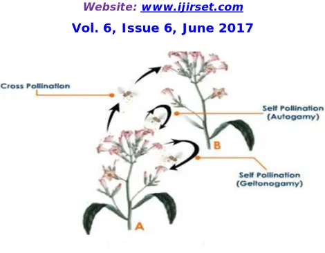
Pollination The reproduction in plants happens by union of the gametes. The pollen grains produced by male gametes and ovules borne by female gametes are produced by different parts and it is essential that the pollen has to be transferred to the stigma for the union. This process of transfer and deposition of pollen grains from anther to the stigma of flower is pollination. The process of pollination is mostly facilitated by an agent. The pollination is a result of fertilization and it is must in agriculture to produce fruits and seeds [2]. There are two types of pollination:
A. Self-Pollination. B. Cross Pollination.
A. Self Pollination
Figure 3 self pollination
B. Cross Pollination
Cross Pollination occurs when pollen grains are moved to a flower from another plant. The process of cross pollination happens with the help of a biotic or biotic agents such as insects, birds, snails, bats and other animals as pollinators. A biotic pollination is a process where the pollination happens without involvement of external agents. Only about 10% of plants fall in this category. The process of pollination which requires external pollinators is known as Biotic Pollination [2] to move the pollen from the anther to the stigma. Insects play most important role as the pollinators. Insect Pollination occurs in plants with coloured petals and strong odour which attract Honey bees, moths, beetles, wasps, ants and butterflies [1]. The insects are attracted to flowers due to availability of nectar, edible pollen and when insect sits on the flower, the pollen grains stick to the body. When the insect visits another flower, the pollen is transferred to stigma facilitating pollination. The pollination is also facilitated by vertebrates like birds and bats. Flowers pollinated by bats mostly have white colored petals and strong our. The birds usually pollinate flowers with red petals and without our.
C. Flower Pollination Algorithm
Flowering plants flow pollination process inspired Xin-She Yang to develop Flower Pollination Algorithm (FPA) in 2012. For ease, the four rules given below are used [4].
Rule1. Biotic and cross-pollination can be considered processes of global pollination, and pollinators carrying pollen move in a way that confirms to levy flights.
Rule 2. For local pollination, a biotic pollination and self-pollination are used.
Rule 3. Pollinators, like insects develop flower loyalty, which is comparable to the reproduction possibility proportional to the matching of two flowers involved.
Rule 4. Switching or the interaction of global pollination and local pollination can be controlled by a switch probability p[0, 1], slightly biased towards local pollination.
To formulate the updating formulas, these rules have to be changed into correct updating equations. The main steps of FPA, or simply the flower algorithm [4] are illustrated below:
min or max objective f(x), x = (x1, x2 , . . . , xd )
Initialize n flowers or pollen gametes population with random solutions Identify the best solution (g*) in the initial population.
intensive local pollination to common global pollination. To start with, a raw value of p = 0.5 may be used as an initial value. A preliminary parametric study indicated that p = 0.8 may work better for most applications.
V. RESULTS AND DISCUSSIONS
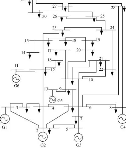
The performance of the Flower Pollination Algorithm (FPA) based method is tested on IEEE-30 bus system considering non smooth cost function. The algorithm is coded in MATLAB 7.6 environment. A Core 2 Duo processor based PC is used for the numerical simulations.
The base load condition is taken for the simulation and the system bus and line data are taken from. The system parameters shown in table 1.Bus 1 is the slack bus and the line data and bus data are on 100MVA basis. The algorithm is run for 500 iterations with 30 as the population size and proximity Probability as 0.8.
Figure 4.Single line diagram of IEEE 30 Bus System
The parameters and the generator cost coefficients of the test system are given in Table 5.1 and Table 5.2.
Table 1 Parameter of the IEEE - 30 bus system
Sl .No Parameter 30-bus system
1 Buses 30
2 Branches 41
3 Generator 6
4 Shunt capacitors 2
5 Tap-Changing
transformer 4
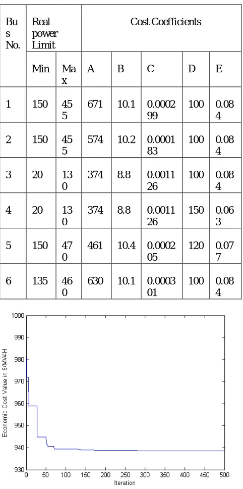
Table 2 Generator cost coefficient for IEEE-30 bus system
Figure5 Convergence behavior of FPA Bu
s No.
Real power Limit
Cost Coefficients
Min Ma x
A B C D E
1 150 45 5
671 10.1 0.0002 99
100 0.08 4
2 150 45 5
574 10.2 0.0001 83
100 0.08 4
3 20 13 0
374 8.8 0.0011 26
100 0.08 4
4 20 13 0
374 8.8 0.0011 26
150 0.06 3
5 150 47 0
461 10.4 0.0002 05
120 0.07 7
6 135 46 0
630 10.1 0.0003 01
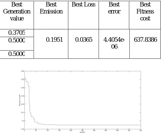
Table 3 NOxEMISSION COEFFICIENTS
Best Generation
value
Best Emission
Best Loss Best error
Best Fitness
cost
0.3705
0.1951 0.0365 4.4054e-06
637.8386 0.5000
0.5000
Figure6 Convergence behavior of EC
VI. CONCLUSION
In this work, a new bio inspired algorithm is implemented for different ELD problems. The numerical results clearly show that the proposed algorithm gives better results. The FPA optimization algorithm outperforms the other recently reported algorithms. The strength of the algorithm is proved in all the three different types of ELD problems. The three objective functions are entirely different in nature and require algorithms are different strengths and hence it can be said that the algorithm is could be suitable for different power system optimization problems. It is obvious from the convergence quality of FPA algorithm in different objectives, the robustness of the algorithm is proved. The algorithm is easy for implementation and can be coded in any computer language. Power system operation optimization problems can be attacked with this algorithm. Power system operators can use this algorithm for various optimization tasks.
REFERENCES
[1] J.B.Park, K.S.Lee, K.Y.Lee, “A particle swarm optimization for economic dispatch with non-smooth cost functions”, IEEE Trans. Power systems, vol.20, Feb.2005.
[2] Sayah S, Zehar K, “Modified Differential Evolution Algorithm for Optimal Power Flow with Non-smooth Cost Functions”, Energy Conversion and management, Vol. 49, No. 11, pp. 3036–3042, 2008.
[3] A. Chakrabarti, S. Halder, Power System Analysis: Operation and Control, Prentice-Hall of India, New Delhi, 2006
[4] Baykasoglu Adil,Ozabakir Lale,Tapkan Pinar, “Artificial Bee Colony and its Application to Generalised Assignment Problem”, I-Tech Education and Publication, 2007.
[5]Willmer P, “Pollination and Floral Ecology”, Princeton University Press.2011
[6] S.Sakthivel, D.Mary “Reactive Power Optimization for Voltage Stability Limit Improvement Incorporating TCSC Device through DE/PSO under Contingency Condition”, IU-Journal of Electrical and Electronics Enginering, Vol. 12, No. 1, pp. 1419-1430, 2012.
[7]Dhayalini. K, Sathiyamoorthy. S & Christober Asir Rajan. C 2014, ‘Genetic algorithm for the coordination of wind thermal dispatch’ , Przeglad Elektrotechniczny,Poland,vol.2014,no.9,pp.45-48.(Impact factor:0.244)
[8] Xin-She Yang, “Book Nature Inspired Optimization Algorithm”, Elsevier,2104
[9] Xin-She Yang, Mehmet Karamanoglu, Xingshi He, “Multi-objective Flower Algorithm for Optimization”, ICCS 2013, Elsevier.
[11]Dhayalini. K, Sathiyamoorthy. S & Christober Asir Rajan. C 2014, ‘Hybrid Evolutionary Particle Swarm optimization for the coordination of wind thermal generation dispatch’ ,Applied Mechanis and Materials, Switerland, vol.573,pp.684-689.
[12] D Karaboga, Technical Report-TR06, “An Idea Based on Honey Bee Swarm for numerical Optimization”, Erciyes University, 2005 [13] Kamalam B, Karnan M, “A Comprehensive review of ABC Algorithm”, IJCT, Volume 5, No:1, 2013.
[14] Osama AbdelRaouf, Ibrahim El-Henawy and Mohamed Abdel-Baset, “A Novel Hybrid Flower Pollination Algorithm with Chaotic Harmony Search for Solving Sudoku Puzzles”, Journal of Modern Education and Computer Science, 2014, pp 38-44.
[15] Dhayalini. K, Sathiyamoorthy. S & Christober Asir Rajan. C 2014,Evolutionary Programming based Optimal Wind and Thermal Generation Dispatch with valve point effect’, International Review on Modelling and Simulations,Italy,vol.7,no.4,pp.598-604.
[16] A. J. Wood, and B. F. Wollenberg, "Power Generation, Operation, and Control", New York: John Wiley & Sons, Inc., 1984. [17] Kennedy J. and Eberhart R “Swarm Intelligence”, Academic Press, 1st ed., San Francisco, CA: Morgan Kaufmann, 2001.
[18] Ding, T., Bo, R., Gu, W., Sun, H. “Big-M Based MIQP Method for Economic Dispatch With Disjoint Prohibited Zones”, IEEE Transactions on Power Systems, Vol. 29 , No. 2 pp. 976 – 977, 2013.
[19] N. Sinha, R. Chakrabarti, and P. K. Chattopadhyay, “Evolutionary programming Techniques for economic load dispatch”, IEEE Trans. Evol. Comput, vol. 7, pp. 83–94, Feb. 2003.
[20] B.H.Chowdhury and S.Rahman,"A review of recent advances in economic dispatch ",IEEE Trans. Power Systems,Vol.5,no.4,pp.1248-1259,Nov.1990.
[21] Abido M. A , “Optimal design of power-system stabilizers using particle swarm optimization,” IEEE Trans. Energy Conv., vol. 17, no. 3, pp. 406– 413, Sept. 2002.
[22] Kassabalidis I. N , M. A. El-Sharkawi, R. J. Marks, L. S. Moulin, and A. P. A. da Silva, “Dynamic security border identification using enhanced particle swarm optimization,” IEEE Trans. Power Syst., vol. 17, pp. 723–729, Aug. 2002.
[23] K.P. Wong, Y.W. Wong, Genetic and genetic/simulated – annealing approaches to economic dispatch, IEE Proc. Gener. Transm. Distrib. 141 (5) (1994) 507– 513.
[24]K.P.Wong,C.C.Fong,Simulatedannealingbasedeconomicdispatchalgorithm, IEE Proc. C (Gener. Transm. Distrib.) 140 (6) (1993) 509–515. [25] Dhayalini. K, 2016 , “Optimization of Wind Thermal Coordination Dispatch using FPA, Journal of Advances in Chemistry, Vol.12, No:16 pp 4963-4970.
[26] W.M.Lin,F.S.Cheng,M.T.Tsay,An improved Tabu search for economicdispatch with multiple minima, IEEE Trans. Power Syst. 17 (1) (2002) 108–112.
[27] J. Cai, X. Ma, L. Li, Y. Yang, H. Peng, X. Wang, Chaotic ant swarm optimization to economic dispatch, Electr. Power Syst. Res. 77 (10) (2007) 1373–1380.