DOI: 10.1534/genetics.108.099309
Statistical Mechanics and the Evolution of Polygenic Quantitative Traits
N. H. Barton*
,†,1and H. P. de Vladar
‡*Institute of Evolutionary Biology, University of Edinburgh, Edinburgh EH9 3JN, United Kingdom,†Institute of Science and Technology Austria, 3400 Klosterneuberg, Austria and‡Theoretical Biology Group, University of Groningen, 9751 NN, Haren, The Netherlands
Manuscript received December 2, 2008 Accepted for publication December 13, 2008
ABSTRACT
The evolution of quantitative characters depends on the frequencies of the alleles involved, yet these frequencies cannot usually be measured. Previous groups have proposed an approximation to the dynamics of quantitative traits, based on an analogy with statistical mechanics. We present a modified version of that approach, which makes the analogy more precise and applies quite generally to describe the evolution of allele frequencies. We calculate explicitly how the macroscopic quantities (i.e., quantities that depend on the quantitative trait) depend on evolutionary forces, in a way that is independent of the microscopic details. We first show that the stationary distribution of allele frequencies under drift, selection, and mutation maximizes a certain measure of entropy, subject to constraints on the expectation of observable quantities. We then approximate the dynamical changes in these expectations, assuming that the distribution of allele frequencies always maximizes entropy, conditional on the expected values. When applied to directional selection on an additive trait, this gives a very good approximation to the evolution of the trait mean and the genetic variance, when the number of mutations per generation is sufficiently high (4Nm.1). We show how the method can be modified for small mutation rates (4Nm/ 0). We outline how this method describes epistatic interactions as, for example, with stabilizing selection.
P
REDICTING the evolution of quantitative charac-ters from first principles poses a formidable chal-lenge. When multiple loci contribute to a quantitative characterz, the effects of selection, mutation, and drift are difficult to predict from the observed values of the trait; this is true even in the simplest case of additive effects. The fundamental problem is that the distribu-tion of the trait depends on the ‘‘microscopic details’’ of the system, namely the frequencies of the genotypes con-tributing to the trait. In an asexual population, long-term evolution depends on the fittest genotypes, which may currently be very rare. In sexual populations—the focus of this article—new phenotypes are generated by recombination in a way that depends on their genetic basis. If selection is not too strong, we can assume Hardy–Weinberg proportions and linkage equilibrium (HWLE): this is a substantial simplifica-tion, which we make throughout. Even then, however, we must still know all the allele frequencies, and the effects of all the alleles on the trait, to predict the evolution of a polygenic trait. In this article, we seek to predict the evolution of quantitative traits without following all the hidden variables (i.e., the allele frequencies) that determine its course.For this purpose, several simplifications have been proposed. The central equation in quantitative genetics
is that the rate of change of the trait mean equals the product of the selection gradient and the additive genetic variance (Lande1976). This simple prediction
can be surprisingly accurate, since the genetic variance often remains roughly constant for some tens of gen-erations (Falconer and Mackay 1996; Barton and
Keightley 2002). However, we have no general
un-derstanding of how the genetic variance evolves or, indeed, what processes are responsible for maintaining it (Bu¨ rger et al. 1989; Falconer and Mackay 1996;
Barton and Keightley 2002). Even if we take the
simplest view, that variation is maintained by the opposition between mutation and selection, the long-term dynamics of the genetic variance still depend on the detailed distribution of effects of mutations.
Lande (1976), following Kimura (1965),
approxi-mated the distribution of allelic effects at each locus as a Gaussian distribution. However, this is accurate only when many alleles are available at each locus and when mutation rates are extremely high (Turelli 1984).
Bartonand Turelli(1987) assumed that loci are close
to fixation, but again this approximation has limited application: in particular, it cannot apply when one allele substitutes for another. Some progress has been made by describing a polygenic system by the moments of the trait distribution (Barton 1986; Barton and
Turelli 1987, 1991; Turelliand Barton1990). For
additive traits, a closely related description in terms of the cumulants is a more natural way to represent the effects of selection (Bu¨ rger1991, 1993; Turelliand 1Corresponding author:Institute of Science and Technology Austria, Am
Barton 1994; Rattray and Shapiro 2001). These
transformations are exact and quite general: they pro-vide a natural description of selection and recombina-tion and extend to include the dynamics of linkage disequilibria as well as allele frequencies. A moment-based description provides a general framework for exact analysis of models with a small number of genes and for approximating the effects of indirect selection (Barton1986; Bartonand Turelli1987; Lenormand
and Otto 2000; Kirkpatrick et al. 2002; Roze and
Barton 2006); for some problems, simply truncating
the higher moments or cumulants can give a good ap-proximation (Turelliand Barton1990; Rouzineet al.
2007). However, results are sensitive to the choice of approximation for higher moments, and so the approx-imation is to this extent arbitrary. The equations must be truncated ‘‘by hand,’’ guided by mathematical trac-tability rather than biological accuracy.
The fundamental problem is to find a way to ap-proximate the ‘‘hidden variables’’ (in this context, the allele frequencies), but we cannot hope to do this in complete generality. Even with simple directional selec-tion on a trait, the pattern of allele frequencies depends on the frequencies of favorable alleles that may be ex-tremely rareðp>1Þand that will takeð1=sÞlogðð1=pÞÞ
generations to reach appreciable frequency. Thus, undetectably rare alleles can shape future evolution, without much affecting the current state. Figure 1 shows an example where the trait mean changes as three alleles sweep to fixation at different times and rates. By choosing initial frequencies and allelic effects appro-priately, we could produce arbitrary patterns of trait evolution. We can hope to make progress only in situations where the underlying allele frequencies can be averaged over some known distribution, rather than taking arbitrary values.
Despite this fundamental difficulty, progress can be made in two ways. First, we can include random drift and follow the distribution of allele frequencies, rather than the deterministic evolution of a single popula-tion. Then, we can hope that the distribution of allele frequencies, conditional on the observed trait values, will explore the space of possible states in a predictable way. Second, we can allow selection to act only on the
observed traits and assume that the distribution of allele frequencies spreads out to follow the stationary distri-bution generated by such selection. That makes it much harder (and perhaps impossible) for populations to evolve into an arbitrary state with unpredictable and idiosyncratic properties. There is an analogy here with classical thermodynamics, in which molecules might start in a special state, such that after some time they concentrate in a surprising way: all the gas might rush to one corner, for example. However, if all states with the same energy are equally likely, this is extremely improbable.
An approach along these lines was proposed by Pru¨ gel-Bennettand Shapiro(1994, 1997), Rattray
(1995), and Pru¨ gel-Bennett (1997), as a general
framework for approximating the dynamics of poly-genic systems. Pru¨ gel-Bennett and Shapiro (1994,
1997), Rattray (1995), and Pru¨ gel-Bennett(1997)
drew on analogies with statistical physics to propose an elegant approach to approximating polygenic systems. The distribution of microstates is chosen as that which maximizes an entropy measure (see alsovanNimwegen
and Crutchfield2000; Pru¨ gel-Bennett2001; Rogers
2003). Pru¨ gel-Bennett and Shapiro (1994, 1997),
Rattray(1995), and Pru¨ gel-Bennett(1997) define
an entropy that is maximized by a multinomial allele frequency distribution, which is sharply peaked around equal allele frequencies. Thus, the procedure is to assume maximum polymorphism, subject to con-straints on the trait distribution. This averaging yields a generating function from which observables (e.g., mean values, variance, and higher moments, as well as correlations) can be obtained. This leads to good approximations for a variety of problems, including mul-tiplicative selection, pairwise epistasis, and stabilizing selection (Rattray 1995); it describes the dynamics
of an arbitrary number of observable variables and pro-vides a consistent way to deal with hidden microscopic variables.
In this article, we use procedures analogous to statistical thermodynamics, but adapted to population genetics. First, we use an information entropy measure, SH, which is derived from population genetic consid-erations and ensures an exact solution at statistical equilibrium. This measure, which is proportional to the quantity H, defined by Boltzmann (1872), was
proposed by Iwasa(1988) and independently by Sella
and Hirsh (2005); see N. H. Barton and J. B. Coe
(unpublished data). Second, we choose to follow a set of observable quantities that includes all those acted on directly by mutation and selection. This reveals a natural correspondence between the observables and the evo-lutionary forces that act on them, which is analogous to extensive and intensive variables in thermodynamics (N. H. Bartonand J. B. Coe, unpublished data). These
two innovations allow us to set out the method in a very general way.
Figure1.—The frequency of favorable alleles at three loci (left) and the mean of an additive trait,z(right). Initial fre-quencies are 105, 106, 107, and effects on the trait are 1, 2,
1
2, so thatz¼p112p2112p3; the selection gradient isb¼0.01
Throughout, we make the usual approximations of population genetics, that populations are at HWLE and that drift, mutation, and selection are weak. Linkage equilibrium is justified if selection and drift are not only weak (s;1=2N>1) but also weak relative to recombina-tion (s; 1=2N>r). We also assume only two alleles at each locus. These assumptions allow us to describe populations solely in terms of allele frequencies atnloci
ð~p¼p1;. . .;pnÞ and to use the continuous-time
diffu-sion approximation.
We begin by analyzing the stationary distribution, showing the analogy with thermodynamics. Iwasa
(1988) showed that the free fitness, which is the sum of the log mean fitness and the information entropy SH(logðWÞ1ð1=2NÞSH), always increases through time
and reaches a maximum at the classic stationary dis-tribution of allele frequencies under mutation, selection, and drift,
cð~pÞ ¼Z1W2NY n
i¼1
ðpiqiÞ4Nm1; ð1Þ
wherepi(i¼1,. . .,n) are the allele frequencies atnloci, qi¼1pi,Nis the number of diploid individuals,W is the mean fitness, andmis the mutation rate (Wright
1937). The normalizing constantZplays a key role; it is
analogous to the partition function in statistical me-chanics and acts as a generating function for the quantities of interest, in the sense that its derivatives give the expectations of the macroscopic quantities (Barton1989). We then show how the rates of change
of expectations of observable quantities can be approx-imated by averaging over this stationary distributionc. The crucial assumption here is that the distribution of allele frequencies always has the form of Equation 1. This is accurate provided that the system evolves as a result of slow changes in the parameters, so that it has time to approach the stationary state. By analogy with thermodynamics, such changes are termed revers-ible (Ao2008; N. H. Bartonand J. B. Coe, unpublished
data).
After setting out the method in a general way, we apply it to directional selection on an additive trait. In this simple case, we can give closed-form expressions for the generating function Z and hence for observables
such as the expectations of the trait mean, genotypic variance, genetic variability, and so on. We then show that our approximation to the allele frequency distri-bution gives a good approximation to the dynamical change in the trait distribution, even when selection changes abruptly. However, the method works only for high mutation rates (4Nm . 1) and breaks down when 4Nm,1. Nevertheless, we show how the method can be adapted to the case where 4Nmis small. Finally, we outline the application to cases such as stabiliz-ing selection, where there are epistatic interactions for fitness.
GENERAL ANALYSIS
Defining entropy: The key concept is of an entropy, SH, which measures the deviation of the population from a base distribution f—in this case, the density under drift alone. Entropy always increases as the pop-ulation converges toward f under drift. With selec-tion and mutaselec-tion, a ‘‘free energy’’—the sum of the entropy and a potential function—always increases (Iwasa1988). We show that the stationary distribution
maximizes SH subject to constraints of the expected value of a set of observable quantities. Thus, the dynamics of these quantities can be approximated by assuming that the entropy is always maximized, conditioned on their values.
There is a wide range of definitions, interpretations, and generalizations of entropy (e.g., Renyi1961; Wehrl
1978; Tsallis 1988); these have been applied to
bi-ological systems in various ways. Iwasa (1988)
intro-duced the concept of entropy into population genetics, for a diallelic system of one locus under reversible mu-tation and with arbitrary selection; he also considered a phenotypic model of quantitative trait evolution. Iwasa
(1988) used an information entropy, also known as a relative entropy (Gzyl1995, Chap. 3; Georgii2003),
and defined as
SH½c[
ð
clog c
f dp~: ð2Þ
This is a function of the probability distribution of allele frequencies,c, that evaluates the average entropy of a function with respect to a given base distribution,f, integrated over all possible allele frequencies, denoted by dp~¼ ðdp1dp2 . . .dpnÞ. It can be thought of as
the expected log-likelihood off, given samples drawn from a distributionc; it has a maximum atc¼f, when SH[f]¼0. We denote it by a subscriptHbecause it is essentially the same as the measure introduced by Boltzmann(1872) in hisH-theorem.
The variation of SHwith respect to small changes in
cis
dSH½c ¼
ð
l1log c
f
dcdp~; ð3Þ
where l is a Lagrange multiplier associated with the normalization conditionÐcdp~¼1 (N. H. Bartonand
J. B. Coe, unpublished data) (see supplemental
infor-mation A). Note that becausecis normalized,Ðdcdp~¼
0. With no constraints other than this normalization, settingdSH¼0 implies that the entropy is at an extreme only ifc¼f; this is a unique maximum.
frequencies,c, that maximizes the entropy,SH[c], given constraints on the expected values of these observables, ÆAjæ:
ÆAjæ¼
ð
Ajcdp~: ð4Þ
With these constraints, the extremum of Equation 3 is calculated by including the Lagrange multipliers asso-ciated with theAj’s, defined for convenience as2Naj:
ð
l1log c
f X
j
2NajAj
!
dcdp~¼0: ð5Þ
At the extremum, the term in parentheses should be zero. This implies that the distribution that maxi-mizes entropy, subject to constraints, is the Boltzmann distribution
cME¼fZexp X j
2NajAj
" #
¼fZexp 2N~aA~
h i ; ð6Þ
where we have expressed the Lagrange multiplierl as
Z¼exp(l) and chooseZto normalize the distribution.
We show later thatZ is a generating function for the
moments of the observables,Aj. It will play a major role in our calculations:
Z¼
ð
fexp 2h Nð~a~AÞidp~: ð7Þ
We show that under directional selection and muta-tion theajcan be identified with the set of selection coefficients and mutation rates and the Aj with the quantities on which selection and mutation act (e.g., trait mean and genetic variability). The potential func-tion PjAjaj ¼~aA~ consists of the log-mean fitness, logðWÞ, plus a term representing the effect of
muta-tion, 2mPjlogðpjqjÞ. Then, Equation 6 gives the classical stationary density of Equation 1. (Note that although ~aA~ must equal the potential function, which includes all evolutionary processes, apart from drift, we still have some freedom to separate this into components in a variety of ways. For example, di-rectional selection on a set of traits could be repre-sented by almost any linear basis. Nevertheless, there will usually be a natural set of components that represent different evolutionary processes. In addi-tion, we are free to include additional observables that are not necessarily under selection, and so haveai¼0. These extra degrees of freedom will improve the ac-curacy of our dynamical approximations.)
Note that there is an alternative measure of entropy, SV, defined by the log density of states that are con-sistent with macroscopic variablesÆA~æ(Barton 1989).
N. H. Bartonand J. B. Coe(unpublished data) discuss
the relation betweenSVandSHand show that these two measures converge when the distribution clusters close to its expectation.
The generating function, Z: The normalizing
con-stant Z, which is a function of~a, acts as a generating
function for quantities of interest. Differentiating with respect to (w.r.t.) 2N~awe find that
@logðZÞ
@ð2NajÞ ¼ÆAjæ: ð8Þ
Differentiating w.r.t. population size,
@logðZÞ
@ð2NÞ ¼Æ~aA~æ: ð9Þ
Differentiating again w.r.t. the~agives the covariance between fluctuations in theA~:
@2logðZÞ
@ð2NajÞ@ð2NakÞ ¼CovðAj;AkÞ[Cj;k: ð10Þ
This covariance matrix, which we denoteC, plays an important role in the dynamical approximation (Le
Bellacet al.2004, p. 64).
Analyzing the dynamics: As the system moves away
from stationarity, it will not in general follow precisely the distribution that maximizes entropy. [This can be seen by substituting the maximum entropy distribution from Equation 6 with time-varying parameters ~aðtÞ as a trial solution to the diffusion equation]. However, the distri-bution of microscopic variables may nevertheless stay close to a maximum entropy distribution (Nicolisand
Prigogine1977; DeGrootand Mazur1984; Goldstein
and Lebowitz 2004). Our key assumption is that the
macroscopic variables change slowly enough that the system is always close to a local equilibrium.
We show that the Lagrange multipliers,~a, correspond to forces that act on the observables, A~: directional selection acts on the trait mean, mutation on a measure of genetic diversityU(see below), and so on. Crucially, we assume that changes occur solely through changes in the parameters ~a; arbitrary perturbations that act di-rectly on the allele frequencies could have arbitrary effects (as, for example, in Figure 1).
Assume that changes in allele frequency are deter-mined by a potential function~aA~, which can be writ-ten as a sum of componentsakAk. [In physics, energy acts as a potential; in population genetics, mean fitness plays an analogous role; it defines an adaptive landscape such that allele frequencies and their means change at rates proportional to the fitness gradient (Wright
1967; Lande1976).] Our method works only for systems
whose dynamics can be described by a potential in this way (although see Ao2008). In an infinitesimal timedt,
Ædpiæ¼ piqi
2
@ð~aA~Þ @pi
; ð11aÞ
Ædpidpjæ¼0 fori6¼j; ð11bÞ
Ædpi2æ¼piqi
2N : ð11cÞ
The first equation, forÆdpæ, is just Wright’s (1937)
formula for selection, modified to include mutation. The variance of allele frequency fluctuations, hdp2i, is
the standard formula for random drift. Under the diffusion approximation, this leads to the stationary distribution of Equation 1, provided that the base dis-tribution is defined as
f¼ Y
n
i¼1
piqi
!1
: ð12Þ
Under the diffusion approximation, the rate of change ofÆAjæis
@ÆAjæ
@t ¼
Xn
i¼1 @Aj
@pi Ædpiæ1
1 2
Xn
i¼1 Xn
k¼1 @2Aj
@pi@pk
Ædpidpkæ
¼X
k
Bj;kak1 1
2NVj; ð13Þ
where
Bj;k¼
Xn
i¼1 @Aj
@pi piqi
2
@Ak
@pi
* +
and Vj ¼
Xn
i¼1
piqi 2
@2Aj
@pi2
* +
:
ð14Þ
This relationship is exact, provided that the matrixB and the vectorVare evaluated at the current distribution of allele frequencies. Equation 13 can also be derived directly, by making a diffusion approximation to multi-variate observables, where the deterministic terms are ai ¼Pkð@Aj=@piÞðpiqi=2Þak, and the diffusion terms are bi¼ ffiffiffiffiffiffiffiffiffiffiffiffiffiffiffiffiffipiqi=2N
p
(Ewens 1979; Gardiner 2004). If our
system is described by only one observable, we directly recover the formula derived by Ewens(1979, pp. 136–137).
The local equilibrium approximation:In general, as the system moves away from stationarity, it will not precisely follow the distribution that maximizes entropy. However, the distribution of microscopic variables may nevertheless stay close to a maximum entropy distribu-tion if the macroscopic variables change slowly enough such that the system remains close to a local equilibrium at all times (Prigogine 1949; Klein and Prigogine
1953; Nicolis and Prigogine 1977; De Groot and
Mazur1984; Goldsteinand Lebowitz2004).
We now approximateBj,kandVjbyB*i;k,Vj*, assuming the distribution in Equation 6 is evaluated at~a*. We know that at the stationary state, under parameters~a*,
expectations are constant, and so from Equation 13,
P
kB*j;kak*1ð1=2NÞVj*¼0. Therefore
@ÆAjæ
@t
X
k
B*j;kðaka*kÞ: ð15Þ
The matrix Bj,k is closely related to the additive genetic covariance matrix. Making the link with quantitative genetics is not quite straightforward, because the Aj are arbitrary functions of the allele frequencies and need not be the means of actual traits carried by individuals. Nevertheless, if we do regard them as the means of some quantity, then @Aj/@piis twice the average effect of alleles at locusi. [Since we assume HWLE, average effect is equal to average excess (Falconer and Mackay 1996)]. Therefore,
Bj,k is the expected additive genetic covariance be-tweenAjandAk, the expectation being taken over the distribution of allele frequencies. Moreover, if the ak
contribute to the log-mean fitness (rather than to the component of the potential that describes mutation), then they can be interpreted as selection gradients in the usual way. Equation 15 thus gives the rates of change of the expected trait means as the product of the expected additive genetic covariance, and the difference between the actual selection gradient, ak, and the gradient that would give stationarity at the current expectations, a*k. This interpretation becomes clearer when we consider specific examples, below.
In the theory of nonequilibrium thermodynamics, equations similar to Equation 15 are called phenome-nological equations (vanKampen1957; DeGrootand
Mazur1984, Chap. IV). They were first postulated as
approximations to processes that are close to equilib-rium. In such cases, the variables a* represent the deviation from an equilibrium defined by a. These equations are valid as long as a local equilibrium exists, and (as suggested by Equation 13) it holds in general thatBk,j¼Bj,k(Onsager1931; Prigogine1949).
For theoretical purposes, we can follow either the expectations ÆAjæ themselves or the parametersa*k that would give those expectations at stationarity. In numerical calculations, the latter is more convenient, because that avoids calculating thea*j from theÆAjæ(a tricky inverse problem). The rates of change of thea*kare related to the rates of change of theÆAjævia the matrix@ÆAjæ=@a*k. Now, sinceÆAjæ¼@ logðZÞ=@ 2Na*
k
, we have
@ÆAjæ=@a*k¼2N @
2logðZÞ=@ð2
Na*jÞ@ð2Na*kÞ
h i
¼2NCjk*:
Thus, the relation between theÆAjæand theak* is via the covariance of fluctuations, C*j;k (Equation 10). In matrix notation (equivalent to DeGroot and Mazur
@~a*
@t 1 2N C*
1B* ð~a~a*Þ; ð16Þ
whereCis the matrix of covariances of fluctuations in the A~, and B is analogous to the additive genetic covariance matrix.
Both of these are evaluated at the stationary distribu-tion defined by~a*. For given ~a*, we find the ÆA~æ by integrating using the density in Equation 6, or by application of Equation 8.
DIRECTIONAL SELECTION, MUTATION, AND DRIFT
Analysis:The stationary distribution:We now apply this method to a quantitative trait under directional selec-tion, mutaselec-tion, and drift. We first define a measure of genetic variability (N. H. Barton and J. B. Coe,
un-published data),
U ¼2X
n
i¼1
logðpiqiÞ; ð17Þ
which is 2ntimes the log-geometric mean heterozygosity across loci (plus a constant);nis the number of loci. The rate of change of pi due to symmetric mutation is
mðqipiÞ ¼ ðpiqi=2Þð@ðmUÞ=@piÞ, as required by Equa-tion 11a. Under our assumpEqua-tion of linkage equilibrium, the rate of change of pi due to selection is ðpiqi=2Þ= ð@logðWÞ=@piÞ(Equation 11a). The log mean fitness, logðWÞ, is a natural potential for the system and will be expressed as a sum of componentsA~~a, where the~aare a set of selection coefficients. We deal with the very simplest case of exponential (directional) selection, but note that the derivation applies to any form of selection for which a potential function can be defined—most obviously, the case where genotypes have fixed fitnesses (see supplemental information A and D). If individuals with trait valuezhave fitnessebz, then to leading order in b, the mean fitness isW ¼ebz. Wright’s equilibrium density can then be written in the form of Equation 6, withA~¼ fz;Ugand~a¼ fb;mg:
c¼f
Ze
2Nðbz1mUÞ: ð 18Þ
Thus, the stationary distribution under mutation, selection, and random drift is given by maximizing the entropy subject to constraints on the expected genetic diversity ÆUæ and the expected trait mean Æzæ. The entropy is defined by Equation 2, with baseline distri-butionf¼Qn
i¼1ðpiqiÞ
1
. Then, Equation 18 is the sta-tionary distribution and is equal to Equation 1.
We have shown that a population evolving under mutation, multiplicative selection, and drift will con-verge to a stationary distribution that has maximum entropy,SH, given the expected trait mean and genetic diversity. As we will see below, other forms of selection can be represented by introducing other observables.
Each constrained observable will be conjugated with a natural variable: in this example, the expected meanÆzæ corresponds to the strength of directional selectionb, and the expected diversityÆUæto the mutation ratem. Information about the full distribution of the observ-ables is contained in the normalizing constantZ, which
is a generating function that depends only on the natural variablesaj. In the next section, we calculate an explicit expression for it.
The generating function for an additive trait:We have not yet made any assumptions about the genetic basis of the trait,z; in general, there might be arbitrary dominance and epistasis. We now assume that it is additive, with locusihaving effectgi,
z¼X
n
i¼1
giðXi1X*i1Þ; ð19Þ
whereXiandXi* represent the allelic states (labeled 0 or 1) of the two copies of each of thenloci. With additivity, exponential selection on the trait corresponds to multiplicative selection on the underlying loci. If we average over the population, where pi represents the frequency of theXi¼1 allele, andqi¼1pi, then the mean and genetic variance are
z¼X
n
i¼1
giðpiqiÞ; vz¼2
Xn
i¼1
g2ipiqi: ð20Þ
More than two alleles could be allowed, but only for special mutation rates that give detailed balance (that is, there must be no flux of probability in the stationary state). The normalization functionZcan now be calculated
explicitly, using Equation 7. In this simple case of directional selection on an additive trait, the integrand separates out as a product over allele frequencies, and so
Z¼
ð
exp 2½ Nðbz1mUÞ Y
n
i¼1
piqi
!1
dp~ ð21aÞ
¼Y
n
i¼1 ð1
0
e2Nb giðpqÞðpqÞ4Nm1dp
ð21bÞ
¼Y
n
i¼1 ffiffiffiffi p p
218NmG½4Nm0F1
1
214Nm;ðNbgiÞ
2
ð21cÞ
¼Y
n
i¼1
ðpffiffiffiffipð4NbgiÞð1=2Þ4NmG½
4NmI4Nmð1=2Þð2NbgiÞÞ;
ð21dÞ
whereG() and0F1(,) are the gamma and the
Finding the expectations ÆUæ,Æzæ: The expectations, variances, and covariances ofzandUcan be calculated either by direct integration or by taking derivatives of log(Z) w.r.t. b and m (Equations 8 and 10). Explicit formulas are given in supplemental information A.
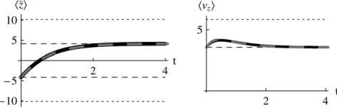
Figure 2 shows how the expected values change for a range of mutation rates and selection pressures, for a population of individuals withnloci of equal effect,gi¼ 1. As selection becomes strong relative to mutation, the alleleX ¼1 tends to fixation, andh iz tends ton (top right of Figure 2). As mutation becomes strong relative to drift, allele frequencies tend to12, and h iz tends to zero (top left of Figure 2). The expected diversity,ÆUæ, increases with mutation rate (bottom left of Figure 2) and decreases slightly with the strength of selection (bottom right of Figure 2). Figure 2 compares the diffusion approximation with the Wright–Fisher model forN¼100. There is close agreement forh iz for all 4Nm
and for ÆUæ when 4Nm . 1. In the discrete model, ÆUæmust be calculated excluding the fixed classes, since Uwould otherwise be infinite. This has negligible effect when 4Nm . 1 because fixation is unlikely. However, when 4Nm,1, there is a substantial probability of being fixed, even when fixed classes must be dropped. Thus, ÆUædepends on population size and differs substantially from the diffusion approximation (compare bottom series of dots with bottom curve in Figure 2, bottom right). The stationary density is still close to the diffusion approximation for polymorphic classes, and so for very large N, when the probability of actually being fixed becomes small ð Ð01=2Np4Nm1dp>1Þ, ÆUæ in the
dis-crete Wright–Fisher model does converge to the diffu-sion approximation. However, for population sizes in the hundreds, there is still a very large discrepancy. We consider the implications of small 4Nmfor the maximum entropy method below.
For an additive trait, and equal allelic effects, the distribution of allele frequencies is the same at each locus, and so this simple case is essentially a single-locus analysis. However, this is no longer the case when we allow unequal allelic effects; more generally, if there is epistasis for fitness, the allele frequency distributions at each locus are no longer independent, and if there is epistasis for the trait, we can no longer treat macro-scopic variables as sums over loci.
Covariances of fluctuations, C, and additive genetic
variance, B: To approximate the dynamics, we need
the covariances of fluctuations, C, and the additive genetic covariance, B, defined above. The matrix C, which gives the variances and covariance ofUandz, is calculated by taking derivatives of the generating function (Equation 10; supplemental information A, Equations A3–A6).
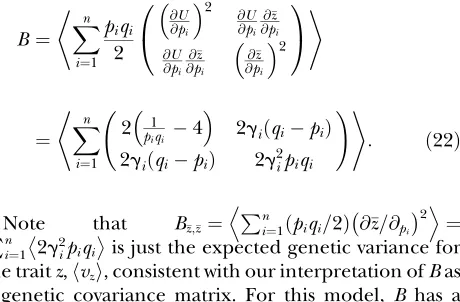
The additive genetic covariance matrixBis defined in Equation 13, in terms of the derivatives@Aj/@pi. For the observablesfU;zg, these are 2f ðqipiÞ=ðpiqiÞ; 2g. Using the relationðqipiÞ2¼14piqi,
B¼ X
n
i¼1
piqi 2
@U @pi 2 @
U @pi
@z @pi
@U @pi
@z @pi
@z @pi 2 0
@
1 A
* +
¼ X
n
i¼1
2 1
piqi 4
2giðqipiÞ
2giðqipiÞ 2g2ipiqi
!
* +
: ð22Þ
Note that Bz;z¼ Pni¼1ðpiqi=2Þ @z=@pi
2
D E
¼ Pn
i¼1 2g 2
ipiqi
is just the expected genetic variance for the traitz,h ivz , consistent with our interpretation ofBas a genetic covariance matrix. For this model, B has a simple form:
B¼
2ð2n14NbÆzæÞ
4Nm1 2Æzæ 2Æzæ 2ðNNmbÞÆzæ
!
: ð23Þ
Remarkably,Bdepends only onh iz and not directly on the distribution of allelic effects, g. Note that the expected genetic variance Ævzæ ¼ 2ðNm=NbÞÆzæ, even with unequal allelic effects. This can be understood by seeing that the rates of change ofÆzædue to mutation,
2mh iz , and due to selection, bÆvzæ, must balance at statistical equilibrium. In the limit where selection becomes weak, both ÆzæandNbtend to zero, and the expected genetic variance tends to a definite limit.
The coefficient BU,U includes the expectation of 1=ðpiqiÞ, which diverges when 4Nm , 1. Because the rate of change depends onBU;Uðm*mÞ(Equation 23), that implies thatm* must be held fixed at its actual value (i.e.,m*¼m). In effect, therefore,ÆUæcan no longer be Figure2.—Dependence ofh iz ; ÆUæonNm,Nb. The solid curves show the diffusion approximation, while the dots show exact values for the Wright–Fisher model with N ¼
included in the approximation. We discuss the implica-tions of this constraint below.
Approximating the dynamics:Evolution of the
expecta-tions:We can now use Equation 15 to approximate the
rates of change of the expectationsÆUæ;h iz :
d dt
ÆUæ Æzæ
2ð2n14NbÆzæÞ
4Nm1 2Æzæ 2Æzæ 2NNmbÆzæ
!
mm* bb*
: ð24Þ
These equations are proportional to the difference between the actual parameters {m,b} and the parame-ters that would give a stationary distribution with the current expectations,fm*;b*g. To iterate these recur-sions, we would need to find fm*;b*g from ÆUæ;Æzæ, which is troublesome. It is more straightforward to work with the rates of change offm*;b*g, which are found by multiplying the rates of change of the expectations (Equation 24) by the inverse of the covariance of fluctuations, C (see Equation 16 and supplemental information A, Equation A6). However, because C depends on the allelic effects in a complex way (see supplemental information A, Equations A3–A5), the full dynamics do depend on the distribution of allelic effects,gi.
In the following sections we test the accuracy of this local equilibrium approximation against two situations: an abrupt change inbormor a sinusoidal change inm
orb. An abrupt change seems the strongest test of our approximation, while a sinusoidal change allows us to find how the accuracy of the approximation decreases as changes become faster. For the moment, we focus on high numbers of mutations (4Nm . 1). We begin by considering the case of equal effects, where the distri-butions at all loci are the same. We also discuss results for the case where most loci have small effect, but some have large effect: the patterns are similar to the symmetric case of equal effects, and so we detail them in supplemental information C. Throughout, we com-pare the approximation with numerical solutions of the diffusion equation: these are close to solutions of the discrete Wright–Fisher model provided that 4Nm . 1 (Figure 3).
Equal allelic effects:If all loci have equal effects on the trait, and if selection acts only on the trait, and not on the individual genotypes, then under directional selec-tion the distribuselec-tion of allele frequencies will be the same at each locus and will be independent across loci. Thus, we need follow only a single distribution, whose time evolution is given either by numerical solution of the diffusion equation or as an expansion of eigenvec-tors (Crow and Kimura 1970, p. 396). However, the
maximum entropy approximation is still nontrivial, even in this highly symmetric case, since it approximates the full distribution by a few degrees of freedom, such as {Æ2 logðpqÞæ,Æpqæ}. Also, note that with other forms of selection, the allele frequency distribution is not
in-dependent across loci: for example, with stabilizing selection populations cluster around states where the sum of allele frequencies is close to the optimum.
Abrupt change in Nb: First, assume that a system is at
equilibrium with evolutionary forcesb0andm0. These
forces are then abruptly changed to new valuesbandm, and the system moves toward its new stationary state. Figure 3 shows that for moderately high mutation rates (Nm¼0.6), and for an abrupt change of selection from Nb ¼ 2 to 12, the approximation is extremely accurate, as compared with the numerical solutions of the diffusion equation. The expected genetic diversity, ÆUæ, increases as the allele frequencies pass through intermediate values, but returns to its original value as Æzæ moves from 2 to 12 (top left). This transient increase in diversity is mainly due to the change in mean allele frequencies: there is only a small transient change inm* (bottom left). The distribution of allele frequen-cies predicted by the approximation is always close to the actual distribution (not shown).
For a lower mutation rate ofNm¼0.3, close to the critical value of Nm¼1
4, the effective mutation rate
hardly changes: it is held close to the actual value of Nm¼0.3 (Figure 4, bottom left). The approximation is still accurate, although there is an appreciable discrep-ancy inÆUæ(Figure 4, top left). For a still lower mutation rate ofNm¼0.1, below the threshold whereBU,Udiverges,
m* must necessarily be held equal to the current mutation rate,m(Figure 5, top left). Then, there is a poor fit to the transient increase in expected diversity, ÆUæ, but the dynamical approximation toÆzæremains accurate (Figure 5, top right). (Because m* must be held fixed at its actual value when 4Nm , 1, ÆUæ is not now included Figure 3.—(Top) Calculation of genetic variability ÆUæ (left) and trait meanÆzæ (right) and over time, with Nm¼
0.6 asNbchanges from2 to12 at timet¼0. The horizontal lines show the stationary values. The solid curves show the ap-proximation, and the dashed curves show numerical solutions to the diffusion equation; these are not distinguishable on this scale. (Bottom) Changes over time in the parameters
in the approximation, which therefore now depends on fitting one variable, rather than two.)
Abrupt change in Nm: Figure 6 shows the effects of an
abrupt change in mutation rate from Nm ¼0.3 to 1. Here, the approximation does poorly when mutation rate increases abruptly, even when 4Nmis always.1 (Figure 6, left side). It does perform better when the mutation rate decreases abruptly, however (t.5 in Figure 6).
Fluctuating selection:As well as examining the effects of an abrupt change in selection, we have also looked at the effects of oscillating selection. If fluctuations are sufficiently slow, then the maximum entropy approxi-mation converges to the exact solution. At the other extreme, when fluctuations are rapid, populations ex-perience an average selective force and behave as if there was a constant selective pressure. The approxima-tion is accurate over the whole range of fluctuaapproxima-tion fre-quencies (supplemental information B).
Unequal allelic effects: So far, we have assumed equal
allelic effects. This ensures that the allele frequency distribution is the same at each locus, so that we are essentially analyzing a single-locus problem. This is not entirely trivial, since we are approximating the full allele frequency distribution by two variables, fh iz ; ÆUæg. However, we now turn to the more challenging case of unequal allelic effects atnloci: now, we are summarizing ndistinct distributions by two variables. We do, however, assume that the allelic effects are known.
We draw allelic effects at 10 loci from a gamma distribution, with mean 1 and standard deviation12:
gi¼ f1:69;1:47;1:15;1:05;1:04;1:03;1:01;0:81;0:500;0:401g:
ð25Þ
The maximum range of the trait is6Pigi ¼10:15,
and the maximum genetic variance is vmax¼
1 2
P10
i¼1g2i ¼11:66. Twenty-five percent of this is contrib-uted by the locus of largest effect, and 54% by the largest three loci.
Figure 7 shows the response of the mean and the genetic variance, as selection changes fromNb¼ 2 to
12, with Nm ¼ 0.3 throughout: the approximation matches well. There is a transient increase in the genetic variance as allele frequencies pass through intermediate values. In Figure 7, the shift is by 3.08 genetic standard deviations.
In supplemental information C, we show how the accuracy of the approximations diminishes as Nm
approaches1
4, in a similar way to Figures 3–5.
LOW MUTATION RATES: 4Nm,1
Failure of the maximum entropy approximation: When the number of mutations produced per genera-tion is small (4Nm,1), populations are likely to be close to fixation. The diffusion approximation still works surprisingly well: it predicts the allele frequency distri-bution accurately even adjacent to the boundaries
ðp¼1=2N; 11=2NÞ. The maximum entropy ap-proximation also makes accurate predictions for the change in trait mean, provided that the mutation rate is kept fixed (Figure 5, top right). However, the approx-imation does not allow changes in m* when 4Nm,1. Formally, the coefficient BU,U(Equation 23) diverges, which implies that the effective mutation rate must always be held equal to the actual mutation rate
ðm*¼mÞ. Thus we lose 1 d.f. from the dynamics. What causes this pathological behavior?
The key point is that near the boundary, the allele frequency distribution changes on a much faster time-scale than in the center: the characteristic timetime-scale of random drift is determined by the number of copies of the allele in question. Thus, the shape of the distribution at the center and the shape at the edge are uncoupled, so that it may be impossible to adequately approximate the whole distribution as being close to the stationary state. Near the boundaries, selection is negligibly slow relative Figure4.—The accuracy of the approximation forNm¼
0.3.Nbchanges from0.7 to10.7 at timet¼0. Otherwise, details are as in Figure 3.
to mutation and drift, and the allele frequency distribu-tion rapidly takes the formp4Nm1, even while the bulk of
the distribution remains unchanged (Figure 8). For example, suppose that 4Nmchanges from,1 to.1. The density at the boundaries immediately falls to zero, and the distribution takes on a two-peaked shape that cannot be approximated by any of the family of stationary distributions. Conversely, when 4Nm falls below the threshold, small singularities immediately develop at the boundaries, representing fixed populations, but it takes a long time for the bulk of the population to approach fixation. This asymmetry explains why the maximum entropy approximation is much more accu-rate when 4Nmfalls than when it rises (Figure 6,t.5). We can gain some insight by analyzing the limit of 4Nm/0, when populations are almost always fixed for one of the 2ngenotypes. With directional selection, the
probability of fixation of one or the other allele is inde-pendent across loci and equalsPi¼1=ð11expð4NbgiÞÞ, where gi is the effect of alleles at the ith locus. Pop-ulations will jump from fixation for ‘‘0’’ to ‘‘1’’ as a result of the fixation of favorable mutations, at a rate 4Nmbgi=ð1expð4NbgiÞÞ, and in the opposite di-rection due to fixation of deleterious alleles, at a rate that is slower by a factor expð4NbgiÞ. In this simple case, it is easy to write down the dynamics at each locus,
dPi
dt ¼4Nmbgi
Qi 11e4Nbgi
Pie4Nbgi 11e4Nbgi
¼4NmbgiðPˆiPiÞ
ðPˆiQˆiÞ; wherePˆi¼ 1 11e4Nbgi;
ð26Þ
noting that this does have a sensible limit asb/0:@tP¼ m(12P), which is correct for neutral alleles. The trait mean changes as
dÆzæ
dt ¼4Nmb
Xn
i¼1
2g2iðPˆiPiÞ
ðPˆiQˆiÞ: ð27Þ
The maximum entropy approximation simplifies the problem by assuming that the Pi always follow a stationary distribution, determined by a single parame-ter b*, with Pi ¼1=ð11expð4Nb*giÞÞ. Thus, pro-vided we know the allelic effects, we can deduce thePi from the observedh iz , without knowing the distribution at thenloci individually. From Equation 24, assuming thatm¼m*, we have
dÆzæ
dt ¼2
Nm
Nb*Æzæðbb*Þ: ð28Þ
This can be understood by seeing that at equilibrium, selection must balance mutation, so that b*gihpiqii ¼ mhpiqii at each locus if the Pi follow a stationary distribution with parameterb*. The rate of change of the trait mean is
X
i 2ðbg2
iÆpiqiæmgiÆpiqiæÞ
¼X
i 2m
b*giÆpiqiæ2mÆzæ¼2mÆzæ b b* 1
;
equal to Equation 28.
It is easy to show that the maximum entropy approx-imation, Equation 28, converges to the exact solution, Equation 27, for smallNbgi; this is confirmed by Figure 9, forNb¼0.2, in an example with equal effects,gi¼1. However, for stronger selection (Nb¼2, thick lines in Figure 9), the maximum entropy approximation under-estimates the initial rate of increase. That is because the approximation is that the initial state, in whichPi¼0.02 at all loci, is caused by strong selection against the 1 allele; such selection would necessarily cause low stand-ing variation, and so the prediction is for a slow response when the direction of selection is reversed. However, as soon as selection is reversed, populations fix new favor-able mutations at a rate that is independent of the previous standing variation. Thus, the method that led Figure 6.—The mutation rate increases abruptly from
Nm ¼ 0.3 to Nm ¼ 1 at t ¼ 0 and then changes back at t¼5; throughout,Nb¼1. The horizontal dashed lines show values at the stationary states, the dashed curves show numer-ical solutions of the diffusion equation, and the solid curves in the top row show the approximation.
Figure 7.—The accuracy of the approximation with un-equal allelic effects,g, given by Equation 25.Nbchanges from
to Equation 24, which was developed for polymorphic populations, fails as 4Nm/0.
Maximum entropy for 4Nm/0:When mutation is
rare, populations are almost always fixed for one of the 2n genotypes, and an ensemble of populations (or
equivalently, the probability distribution of a single population) evolves as a result of jumps between genotypes, mediated by fixation of single mutations. The stationary distribution is proportional to W2N, multiplied by a factor that reflects the pattern of mutation rates (Iwasa1988; Sellaand Hirsh 2005);
this can be derived as the limit of Equation 1 for small 4Nm(N. H. Bartonand J. B. Coe, unpublished data).
We can go further and apply the maximum entropy method to this process. This gives an approximation for the dynamics of macroscopic quantities such asÆzæ, so that we do not need to follow the full distribution across the 2n genotypes. In the simplest case of directional
selection on an additive trait, with equal allelic effects, this gives no benefit, since the distribution of fixation probability is independent across loci and, moreover, is the same at each locus: the problem therefore involves just a single variable,P. However, with unequal effects, the maximum entropy approximation does give a useful simplification, since we do not need to follow the individual Pi. With epistasis for fitness or for the trait, the advantage would be greater, since we would then avoid following the full probability distribution, across the 2n
genotypes. (Note that in the limit of 4Nm/0, the
model applies regardless of the pattern of recombina-tion, because only one locus evolves at a time.)
We now apply the maximum entropy approximation to directional selection on an additive trait, assuming that 4Nm/0, but allowing for unequal allelic effects,gi. (This is distinct from the previous section, since we now apply maximum entropy to the limiting system, rather than apply the limit of 4Nm/0 to the full maximum entropy approximation.) The system is described by a single local variable, b*, defined implicitly by Æzæ¼Pigitanh 2½ Nb*gi; the assumption is that at each locus,ðPiQiÞ ¼tanh 2½ Nb*gi, as if the ensemble were at a local stationary state under a selection gradientb*. Thus
dÆzæ
dt ¼
X
i
2gidPi
dt
¼X
i
2gi 4Nmbgi Qi
11e4Nbgi
Pie4Nbgi 11e4Nbgi
¼4NmbX
i
g2i 1tanh 2½ Nb*gi
tanh 2½ Nbgi
:
ð29Þ
It is easier to work in terms of b*. Multiplying by db*=dz, we obtain a closed equation forb*:
db*
dt ¼2mb
P
ig2i 1
tanh 2½Nb*gi
tanh 2½Nbgi
P
ig2i 1tanh 2½ Nb*gi2
: ð30Þ
When selection is weak 2ð Nb*gi>1Þ, Equation 29 simplifies to 4NmPig2
iðbb*Þ. Since 2Nb*
P
ig
2
i
z
h iin this limit, this converges to 4NmPig2
i
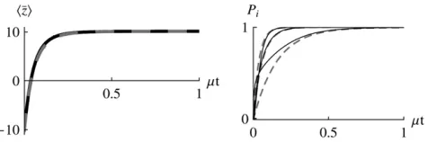
b2mh iz . The exact solution, Equation 27, converges to the same Figure9.—Comparison between the exact solution (Equa-tion 27) and the maximum entropy approxima(Equa-tion (Equa(Equa-tion 28), in the limit of low mutation rates (4Nm/0). Initially, the probability that a locus is fixed for the ‘‘1’’ allele isP¼0.02 at all loci, so thatÆzæ=n¼ 0:99; all alleles have effectg¼1. Se-lectionNb¼0.2 orNb¼2 is then applied, and the trait mean shifts to a new equilibrium, in which a fractionP¼1/(11
exp(4Nb)) of loci are fixed for the 1 allele. When selection is weak (Nb¼0.2), the maximum entropy approximation is barely distinguishable from the exact solution. However, when selection is strong (Nb¼2), the maximum entropy approxima-tion (dashed lines) underestimates the initial rate of change. Figure8.—Failure of the maximum entropic distribution
limit with weak selection. This is as expected, since when selection is weak, the population approaches a mutation– drift equilibrium, with genetic variance 4NmPig2
i
; the trait mean then changes at a rateð4NmPig2
iÞbdue to selection and2mÆzædue to mutation.
Figure 10 shows an example where selection is strong, changing abruptly fromNb¼ 4 to14. The effects of 10 loci are drawn from a gamma distribution, as in Equation 25. The predictions for the mean are in-distinguishable (Figure 10, left). There are substantial errors in the predictions for the underlying allele frequencies, with the rate of change of alleles of small effect being greatly overestimated (Figure 10, bottom curve at right) and that of alleles of large effect being slightly underestimated. However, these errors almost precisely cancel in their effects on the mean.
DISCUSSION
The maximum entropy approximation:A
fundamen-tal aim of quantitative genetics is to understand the evolution of the phenotype, without knowing the un-derlying distribution of all possible gene combinations. Assuming linkage equilibrium simplifies the problem, which then depends only on the allele frequencies rather than on the full distribution of genotypes. However, if we include random drift, as well as selection and mutation, a full description of the stochastic dynamics requires the distribution of allele frequencies—a formidable task. We know that in general, we cannot predict phenotypic evolution without knowing the frequencies of all the relevant alleles: the future response to selection may depend on the frequencies of alleles that are currently so rare that they have negligible effect on the phenotype and so are essentially unpredictable. To avoid this difficulty, we make the key assumption that selection and mutation act only on observable quantities. Then, the distribution of allele frequencies tends toward a stationary state that depends only on those forces. If selection could instead act on individual alleles, it could send the population into arbitrary states by picking out particular alleles (e.g., Figure 1). Selection on individual alleles would be analogous to Maxwell’s demon, which perturbs individual gas molecules to generate improb-able states that violate the laws of classical thermody-namics (Leffand Rex2003).
Populations tend toward a stationary state that max-imizes entropy—that is, the distribution of allele fre-quencies spreads out as widely as possible, conditional on the average values of the quantities that are acted on by selection and mutation. The maximum entropy approximation to the dynamics amounts to assuming that the allele frequency distribution always maximizes entropy, given the current values of the observed variables, even though those variables may be changing. This approximation converges to the exact solution
when changes in mutation and selection (~a) are slow. However, we find that even if selection abruptly changes in direction, predictions for the trait mean are re-markably accurate.
The analogy between the population genetics of quantitative traits and statistical mechanics is intrigu-ing. As well as suggesting methods for approximating phenotypic evolution, it also helps us to better un-derstand the scope of statistical mechanics, by showing that it does not depend on physical principles such as conservation of energy (Ao2008). Selection can be seen
as generating information, by picking out the best-adapted genotypes from the vast number of possibilities, despite the randomizing effect of genetic drift. This is analogous to the way that a physical system does useful work, despite the tendency for entropy to increase. Such issues are discussed by N. H. Barton and J. B. Coe
(unpublished data) and by H. P.deVladarand I. Pen
(unpublished data). Here, we concentrate on the use of maximum entropy as an approximation procedure.
Provided that the number of mutations, 4Nm, is constant, and not too small, the method accurately predicts the evolution of the trait mean—even when allelic effects vary across loci, and even when selection changes abruptly. This accuracy even when parameters change rapidly is surprising, because the underlying allele frequencies may not be well predicted (e.g., Figure 10). Indeed, Pru¨gel-Bennett, Rattray, and Shapiro make accurate predictions even though they use an arbitrary entropy measure that does not ensure convergence to the correct stationary distribution. Although we believe that our entropy measure is the most natural for quantitative genetic problems, and it does guarantee convergence to the stationary state, it may be that the maximum entropy approximation is an efficient method for reducing the dimensionality of a dynamical system, even when an unnatural measure is used.
Figure10.—The maximum entropy approximation (Equa-tion 29), made assuming that popula(Equa-tions jump between fixed states, gives an accurate prediction for the change in mean (left): this is indistinguishable from the exact solution (Equation 27). The population is initially at equilibrium with directional selection Nb ¼ 4; selection then changes sign abruptly. Allelic effects are given by Equation 25. Predictions for the underlying allele frequencies are less accurate. (Right) Allele frequencies at the locus with the strongest effect
g1¼1:69
The maximum entropy method predicts the full allele frequency distribution from just a few quantities, such as the expected trait mean,Æzæ. We do still need to know the genetic basis of the trait—for an additive trait, we must know the allelic effects. We could hardly expect to predict the evolution of phenotype without knowing anything about its genetic basis. However, we could apply the method knowing just the distribution of allelic effects, which could be estimated in a number of ways: by detection of QTL, from evolutionary arguments about plausible distributions (e.g., Orr2003), or from
the distribution of allele frequencies at synonymous and nonsynonymous sites (e.g., Loeweet al.2006).
Extension to dominance and epistasis: We have
analyzed only the simplest case, of directional selection on an additive trait. An extension to allow dominance is straightforward, since the loci still fluctuate indepen-dently of each other, and the generating function, Z,
can still be written as a product of integrals across loci. Extension to more than two alleles is also possible, but only under the restrictive condition that mutation rates allow for detailed balance and hence for an explicit potential function. Similarly, alleles at different loci may interact in their effect on the trait. If such epistasis involves nonoverlapping pairs of loci, then calculations can still be made, but require integrals over pairs of allele frequencies. Although it is beyond the scope of this article to present such calculations, it is important to point out that, despite the technical difficulties, the method itself is general and as such it does not depend on the selective scheme, epistatic model, number of alleles, etc.
It is relatively straightforward to allow for stabiliz-ing selection on an additive trait. In this case, allele frequency distributions at different loci are no longer independent. However, they are coupled only via a single variable, the trait mean: if this lies above the optimum, then all loci experience selection for lowerz, and vice versa. This simple coupling allows explicit solutions for the stationary distribution and for the rate of jumps between metastable states. These calculations are given in Barton (1989) and Coyne et al. (1997,
Appendix). We outline the maximum entropy approx-imation to the dynamics of stabilizing selection in supplemental information D.
For complex models, involving epistasis between large numbers of genes, calculation of the maximum entropy approximation (i.e., of the matricesB*,C*) by numerical integration would not be feasible. They could still be calculated by a Monte Carlo method: one would fix the parameters~a* and simulate the distribution to determine the expectationsÆA~æ. The matrixC* could be found from the covariance of fluctuations, and the matrixB* from Equation 13. The two matrices, Bð~a*Þ
and Cð~a*Þ, would then give the dynamics on the reduced space of~a*;this would be feasible numerically for two or three variables. Of course, this approach
involves the same kind of computation as a direct simulation. Our claim is that the reduced dynamics will be approached, regardless of the initial allele frequency distribution: the system is expected to move close to the lower-dimensional space defined by the maximum entropy approximation. The implication is that we could predict the evolution of the expectations ÆA~æby a closed set of equations, without knowing the actual allele frequency distribution. This will require that we know the genetic basis and mutability of the trait and that selection acts only on that trait.
Low mutation rates (4Nm,1):We describe mutation
and selection by using a potential function
mU 1logðWÞ, where U ¼2PilogðpiqiÞ, and include the variableh iU together with selected variables such as the expectation of the trait mean, h iz . However, this approach fails to describe the effects of changes in mutation rate when 4Nm,1, because then populations are likely to be close to fixation, in which caseUdiverges. The fundamental problem is that the distribution at the boundaries changes rapidly as mutation rate changes, while the bulk of the distribution does not. We can, however, extend the method to the case where 4Nmis very small, because then populations jump between fixation for one or the other genotype, through the substitution of single mutations. This limit is in fact more general, in that it applies even with linkage or with asexual reproduction. It could be extended to give a more accurate approximation for appreciable 4Nm, by calculating the probability of a jump between states of near fixation, taking into account the polymorphism at other loci (see Barton1989).
Long-term response to selection: A basic and long-standing puzzle in quantitative genetics is the success of artificial selection: in moderately large populations, traits respond steadily to selection for $100 genera-tions, with little change in additive genetic variance and often with concordance between replicates (Barton
and Keightley2002). This is surprising, because the
genetic variance is expected to change as alleles sweep through the population. However, if the distribution of allele frequencies is proportional to (pq)4Nm1, as we
assume, and if 4Nmis small, then the additive genetic variance is expected to stay constant for long periods under directional selection. This is because the baseline distributionf(p)¼(pq)1is uniform when transformed
to a logit scale [i.e.,f(z)¼constant forz¼log(p/q)]. Since log(p/q) increases linearly with time under di-rectional selection, that implies that the increase in genetic variance due to rare alleles increasing to become common is precisely balanced by the decrease due to common alleles approaching fixation. Thus, the re-sponse to standing variation is expected to continue steadily at a rate dh iz =dt¼4NmbPig2
response will continue indefinitely as a result of new mutation, at just the same rate. This is because variation is initially maintained in a balance between mutation and drift; the genetic variance is not affected by di-rectional selection, and so the rate of response stays the same even as it shifts from alleles that were originally present to new mutations.
The stationary density under mutation, selection, and drift has been exploited before to help understand the evolution of quantitative traits (e.g., Keightleyand Hill
1987; Keightley1991). In this article, we have shown
that the dynamics of polygenic traits can be accurately approximated by assuming that the underlying distri-bution of allele frequencies always takes this stationary form. We are now starting to get detailed estimates of the distribution of allele frequencies and of allelic effects on traits and on fitness (e.g., Loeweet al.2006;
Boykoet al.2008): it may be that we will soon be able to
use such data to apply the methods developed here to natural and artificial populations.
We are grateful to Ellen Baake for helping to initiate this project and for her comments on this manuscript. We also thank Michael Turelli for his comments on the manuscript and I. Pen for discussions and support in this project. This project was a result of a collaboration supported by the European Science Foundation grant ‘‘Integrating population genetics and conservation biology.’’ N.B. was supported by the Engineering and Physical Sciences Research Council (GR/T11753 and GR/T19537) and by the Royal Society.
LITERATURE CITED
Ao, P., 2008 Emerging of stochastic dynamical equalities and steady
state thermodynamics from Darwinian dynamics. Commun. Theor. Phys.49:1073–1090.
Barton, N. H., 1986 The maintenance of polygenic variation
through a balance between mutation and stabilizing selection. Genet. Res.49:157–174.
Barton, N. H., 1989 The divergence of a polygenic system under
stabilizing selection, mutation and drift. Genet. Res.54:59–77. Barton, N. H., and P. D. Keightley, 2002 Understanding
quanti-tative genetic variation. Nat. Rev. Genet.3:11–21.
Barton, N. H., and M. Turelli, 1987 Adaptive landscapes, genetic
distance, and the evolution of quantitative characters. Genet. Res.49:157–174.
Barton, N. H., and M. Turelli, 1989 Evolutionary quantitative
ge-netics: How little do we know? Annu. Rev. Genet.23:337–370. Barton, N. H., and M. Turelli, 1991 Natural and sexual selection
on many loci. Genetics127:229–255.
Boltzmann, L., 1872 Further studies on the thermal equilibrium of
gas molecules. Sitzungsber. Akad. Wiss. Wien II66:275–370. Boyko, A., S. Williamson, A. Indap and J. Degenhardt,
2008 Assessing the evolutionary impact of amino acid muta-tions in the human genome. PLoS Genet.4:e1000083. Bu¨ rger, R., 1991 Moments, cumulants and polygenic dynamics.
J. Math. Biol.30:199–213.
Bu¨ rger, R., 1993 Predictions of the dynamics of a polygenic
char-acter under directional selection. J. Theor. Biol.162:487–513. Bu¨ rger, R., G. P. Wagnerand F. Stettinger, 1989 How much
her-itable variation can be maintained in finite populations by muta-tion selecmuta-tion balance. Evolumuta-tion43:1748–1766.
Coyne, J. A., N. H. Barton and M. Turelli, 1997 A critique of
Wright’s shifting balance theory of evolution. Evolution51:643–671. Crow, J. F., and M. Kimura, 1970 An Introduction to Population
Genet-ics Theory.Harper & Row, New York.
DeGroot, S. R., and P. Mazur, 1984 Non-Equilibrium
Thermodynam-ics.Dover, New York.
Ewens, W. J., 1979 Mathematical Population Genetics.Springer-Verlag,
Berlin.
Falconer, D. S., and T. F. C. Mackay, 1996 Introduction to
Quantita-tive Genetics, Ed. 4. Longmans Green, Essex, UK.
Gardiner, C., 2004 Handbook of Stochastic Methods.Springer-Verlag,
Berlin.
Georgii, H., 2003 Probabilistic aspects of entropy, pp. 37–56 in
En-tropy, edited by A. Greven. Princeton University Press, Princeton, NJ.
Goldstein, S., and J. Lebowitz, 2004 On the (Boltzmann) entropy
of non-equilibrium systems. Physica D193:53–66.
Gzyl, H., 1995 The maximum entropy method, pp. 27–40 inSeries
on Advances in Mathematics for Applied Sciences, Vol. 29. World Scientific, Singapore.
Iwasa, Y., 1988 Free fitness that always increases in evolution. J.
Theor. Biol.135:265–281.
Keightley, P. D., 1991 Genetic variance and fixation probabilities
at quantitative trait loci in mutation-selection balance. Genet. Res.58:139–144.
Keightley, P. D., and W. G. Hill, 1987 Directional selection and
variation in finite populations. Genetics117:573–582. Kimura, M., 1965 A stochastic model concerning the maintenance
of genetic variability in quantitative characters. Proc. Natl. Acad. Sci. USA54:731–736.
Kirkpatrick, M., T. Johnsonand N. Barton, 2002 General models
of multilocus evolution. Genetics161:1727–1750.
Klein, G., and I. Prigogine, 1953 Sur la mecanique statistique des
phenomenes irreversibles I. Physica19:74–88.
Lande, R., 1976 Natural selection and random genetic drift in
phe-notypic evolution. Evolution30:314–334.
Le Bellac, M., F. Mortessagne and G. G. Batrouni, 2004
Equi-librium and Non-EquiEqui-librium Statistical Thermodynamics.Cambridge University Press, Cambridge, UK.
Leff, H. S., and A. F. Rex, 2003 Maxwell’s Demon II.Institute of
Phys-ics, Bristol, UK.
Lenormand, T., and S. Otto, 2000 The evolution of recombination
in a heterogeneous environment. Genetics156:423–438. Loewe, L., B. Charlesworth, C. Bartolome and V. Noel,
2006 Estimating selection on nonsynonymous mutations. Ge-netics172:1079–1092.
Nicolis, G., and I. Prigogine, 1977 Self Organization in
Non-Equilibri-um Systems: From Dissipative Structures to Order Through Fluctuations.
John Wiley & Sons, New York.
Onsager, L., 1931 Reciprocal relations in irreversible processes.
I. Phys. Rev.37:405–426.
Orr, H. A., 2003 The distribution of fitness effects among beneficial
mutations. Genetics163:1519–1526.
Prigogine, I., 1949 Le domaine de validite´ de la thermodynamique
des phe´nome`nes irre´versibles. Physica15:272–284.
Pru¨ gel-Bennett, A., 1997 Modelling evolving populations. J. Theor.
Biol.185:81–95.
Pru¨ gel-Bennett, A., 2001 Modeling crossover-induced linkage in
genetic algorithms. Evol. Comp.5:376–387.
Pru¨ gel-Bennett, A., and J. L. Shapiro, 1994 An analysis of genetic
algorithms using statistical mechanics. Phys. Rev. Lett.72:1305–1309. Pru¨ gel-Bennett, A., and J. Shapiro, 1997 The dynamics of a genetic
algorithm for simple random Ising systems. Physica D104:75–114. Rattray, M., 1995 The dynamics of a genetic algorithm under
sta-bilizing selection. Complex Syst.9:213–234.
Rattray, M., and J. Shapiro, 2001 Cumulant dynamics of a
popu-lation under multiplicative selection, mutation, and drift. Theor. Popul. Biol.60:17–32.
Renyi, A., 1961 On measures of entropy and information, pp. 547–
561 inProceedings of the Fourth Berkeley Symposium on Mathematics and Statistical Probabilities, Vol. 1. University of California Press, Ber-keley, CA.
Rogers, A., 2003 Phase transitions in sexual populations subject to
stabilizing selection. Phys. Rev. Lett.90:158103.
Rouzine, I., E. Brunetand C. Wilke, 2007 The traveling-wave
ap-proach to asexual evolution: Muller’s ratchet and speed of adap-tation. Theor. Popul. Biol.73:24–46.
Roze, D., and N. H. Barton, 2006 The Hill–Robertson effect and
the evolution of recombination. Genetics173:1793–1811. Sella, G., and A. E. Hirsh, 2005 The application of statistical physics
Tsallis, C., 1988 Possible generalization of Boltzmann-Gibbs
statis-tics. J. Stat. Phys.52:479–487.
Turelli, M., 1984 Heritable genetic variation via mutation-selection
balance: Lerch’s zeta meets the abdominal bristle. Theor. Popul. Biol.25:138–193.
Turelli, M., and N. H. Barton, 1990 Dynamics of polygenic
char-acters under selection. Theor. Popul. Biol.38:1–57.
Turelli, M., and N. H. Barton, 1994 Genetic and statistical-analyses
of strong selection on polygenic traits: What, me normal? Genetics 138:913–941.
vanKampen, N. G., 1957 Derivation of the phenomenological
equa-tions from the master equation. Physica101:707–719.
vanNimwegen, E., and J. Crutchfield, 2000 Optimizing epochal
evolutionary search: population-size independent theory. Comp. Methods Appl. Mech. Eng.9:171–194.
Wehrl, A., 1978 General properties of entropy. Rev. Mod. Phys.50:
221–260.
Wright, S., 1937 The distribution of gene frequencies in
popula-tions. Proc. Natl. Acad. Sci. USA23:307–320.
Wright, S., 1967 ‘‘Surfaces’’ of selective value. Proc. Natl. Acad. Sci.
USA58:165–172.