Empirical Evaluation of Genetic Clustering Methods Using Multilocus
Genotypes From 20 Chicken Breeds
Noah A. Rosenberg,* Terry Burke,
†,1Kari Elo,
‡Marcus W. Feldman,*
,1Paul J. Freidlin,
§,1Martien A. M. Groenen,**
,1Jossi Hillel,
§,1Asko Ma¨ki-Tanila,
‡,1Miche`le Tixier-Boichard,
††,1Alain Vignal,
‡‡,1Klaus Wimmers
§§,1and Steffen Weigend***
*Department of Biological Sciences, Stanford University, Stanford, California 94305,†Department of Animal and Plant Sciences, Sheffield
University, S10 2TN, United Kingdom,§Department of Genetics, The Hebrew University of Jerusalem, Faculty of Agriculture, Rehovot 76100,
Israel,**Institute of Animal Sciences, Wageningen Agricultural University, 6700 AH Wageningen, The Netherlands,‡Agricultural Research
Centre, Institute of Animal Production, FIN-31600 Jokioinen, Finland,†Institut National de la Recherche Agronomique, Centre de Recherches
de Jouy-en-Josas, 78 352 Jouy-en-Josas Cedex, France,‡‡Institut National de la Recherche Agronomique, Centre INRA de Toulouse, 31326
Castanet Tolosan, France,§§Institute of Animal Breeding Science, Rheinische Friedrich-Wilhelms-Universitat, D-53012 Bonn, Germany and ***Institute for Animal Science and Animal Behaviour, Mariensee, 31535 Neustadt, Germany
Manuscript received March 26, 2001 Accepted for publication August 1, 2001
ABSTRACT
We tested the utility of genetic cluster analysis in ascertaining population structure of a large data set for which population structure was previously known. Each of 600 individuals representing 20 distinct chicken breeds was genotyped for 27 microsatellite loci, and individual multilocus genotypes were used to infer genetic clusters. Individuals from each breed were inferred to belong mostly to the same cluster. The clustering success rate, measuring the fraction of individuals that were properly inferred to belong to their correct breeds, was consistentlyⵑ98%. When markers of highest expected heterozygosity were used, genotypes that included at least 8–10 highly variable markers from among the 27 markers genotyped also achieved⬎95% clustering success. When 12–15 highly variable markers and only 15–20 of the 30 individuals per breed were used, clustering success was at least 90%. We suggest that in species for which population structure is of interest, databases of multilocus genotypes at highly variable markers should be compiled. These genotypes could then be used as training samples for genetic cluster analysis and to facilitate assignments of individuals of unknown origin to populations. The clustering algorithm has potential applications in defining the within-species genetic units that are useful in problems of conservation.
C
HARACTERIZATIONS of the population struc- Population structure assessment has often relied upon ture of species are useful in a variety of contexts. a priorigroupings of individuals on the basis of pheno-Genetic ascertainment of within-species population struc- types or sampling locations. A classification chosen by ture has been widely applied for classifying subspecies, an investigator, however, might not accurately describe for defining intraspecific conservation units, for under- the genetic structure of the populations. Genetically standing events in the history of a species, for identifying similar groups of individuals might be labeled differ-ongoing speciation events, and for testing hypotheses ently due to distinct geography, different phenotypes, about evolutionary processes. In other situations, the or, in the case of human groups, cultural differences; presence of population structure poses a practical nui- however, a high level of geographic, phenotypic, or sance. For example, allele frequencies in reference cultural diversity among a collection of populations groups are central to calculations in forensic studies, need not imply that the groups are genetically divergent. and it is difficult to identify appropriate reference groups Conversely, geographic overlap or phenotypic similarity in structured populations (National Research Coun- may mask underlying genetic variation. Thus, a purely cil1996). In case-control studies that test for statistical genetic analysis using no external information provides associations between a genotype at a particular locus the most direct method of determining population and a phenotype, not taking into account population structure. Only if a correspondence between genetic structure can lead to the false detection of associations and geographic or phenotypic classifications is estab-(e.g.,DevlinandRoeder1999). lished can these characteristics also serve as appropriateclassification tools.
The structurealgorithm (Pritchardet al. 2000)
con-Corresponding author:Noah A. Rosenberg, Program in Molecular structs genetic clusters from a collection of individual
and Computational Biology, University of Southern California, 1042
multilocus genotypes, estimating for each individual the
W. 36th Pl., DRB 155, Los Angeles, CA 90089-1113.
fractions of its genome that belong to each cluster. In
E-mail: [email protected]
1These authors are listed alphabetically. contrast to methods that use genetic distances, sampling
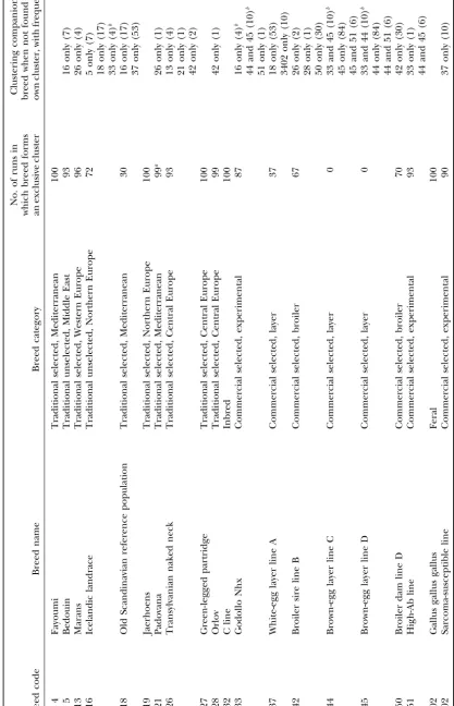
commercial broilers (Broiler dam line D[50],Broiler sire line B locations, hypothesized genetic origins of individuals,
[42]), experimental lines (Godollo Nhx[33],High-Ab line[51], phenotypic information, and the number of genetic
Sarcoma-susceptible line[3402]), and commercial layers ( Brown-clusters do not need to be specified before the algorithm egg layer line C[44],Brown-egg layer line D[45],White-egg layer is applied. With extensive simulations,Pritchardet al. line A[37]); and a highly inbred strain of white leghorn origin
maintained at low population size (C line[32]). (2000) demonstrated that the structure genetic cluster
Markers:Genotypes were used for 27 microsatellite markers analysis method can accurately infer individual
ances-spread across the chicken genome (listed in Table 1). Except tries. For two data sets, one in which two genetic clusters
for ADL278, LEI94, LEI166, LEI194, LEI228, and LEI234, it were inferred and another for which three were inferred, has previously been reported that these markers show high they found that the inferred and expected population levels of polymorphism within and between breeds (Hillel et al. 1999). In general, pairs of markers among these are structures were roughly coincident.
unlinked (seeGroenenet al. 2000 for a map). In this article, we consider the utility of genetic cluster
Genotyping:Genotyping was performed in the laboratories analysis on a large data set for which population
struc-of T. Burke, M. A. M. Groenen, J. Hillel, and S. Weigend, with ture is known, with the aim of making recommendations similar procedures used in all labs. The example procedure about its future uses. We employ a collection of 27-locus that follows is from the laboratory of S. Weigend. PCR products were obtained in a 25-l volume using Ready-To-Go PCR Beads genotypes from 600 individuals representing 20 chicken
(no. 27-9555-01; Amersham Pharmacia Biotech Europe, Frei-breeds. This data set is substantially larger than previous
burg, Germany) and a thermal cycler (Mastercycler; Eppen-data sets on whichstructurehas been applied (
Pritch-dorf, Hamburg, Germany). Two pairs of microsatellite primers
ardet al. 2000;Beaumontet al. 2001;Rosenberget al. were run in one tube. Each PCR tube contained 20 ng of
2001) and it includes individuals from a larger number genomic DNA, 10 pmol of each forward primer labeled with either IRD700 or IRD800 (MWG-Biotech, Ebersberg, Ger-of genetic populations. Importantly, isolation Ger-of the
many), 10 pmol of each unlabeled reverse primer, and 1 mm
breeds in different locations allows us to be sure that, in
tetramethylammoniumchloride. The amplification involved most cases, these breeds have been genetically separated
initial denaturation at 95⬚(1 min), 35 cycles of denaturation from each other for at least 20–50 generations, so that at 95⬚(1 min), primer annealing at temperatures varying be-we can test if cluster analysis successfully uncovers this tween 58⬚ (1 min) and extension at 72⬚ (1 min), followed genetic structure. by final extension at 72⬚ (10 min). Specific DNA fragments produced by amplification were visualized as bands by 8% We first characterize the genetic differences among
PAGE, which was performed with a LI-COR automated DNA the populations. We then demonstrate that genetic
clus-analyzer (LI-COR Biotechnology Division, Lincoln, NE 68504). ter analysis has great ability to correctly ascertain the Electrophoregram processing and allele-size scoring were per-population structure for these data, and we compare formed with the RFLPscan package (Scanalytics, Division of the cluster analysis to a cladogram derived from the CSP, Billerica, MA).
Missing data:The proportion of missing data was 0.8%, and neighbor-joining algorithm. To assess the success of
12 of 27 loci had missing genotypes. For no locus were⬎3.5% clustering as a function of the number of markers, we
of the possible genotypes missing. Missing genotypes were consider subsets of the loci chosen by different criteria
distributed across 88 individuals from 18 breeds. For no breed of variability. We also consider the success of clustering were⬎4.1% of its genotypes missing. Out of 600 individuals, as a function of the number of individuals used per 13 individuals originating from 6 breeds did not have available genotypes at⬎1 locus. These 13 individuals included 1 individ-population. Finally, we discuss recommendations on the
ual that was lacking genotypes at 9 loci and 3 individuals that use of genetic cluster analysis for ascertaining
popula-were missing genotypes at 10 loci. tion structure, for applications in the assignment of
Statistical analysis: Genetic differentiation: For each pair of individuals of unknown origin to populations, and for breeds, allele frequencies were tabulated at each locus, se-identifying genetically distinctive populations. quentially pooling the rarest alleles into one allelic class, until the average frequency for the two breeds exceeded 0.1 for each class. A chi-square association test statistic was computed for each locus, with the number of degrees of freedom equal-MATERIALS AND METHODS
ing one fewer than the number of allelic classes. We counted how many loci produced test statistics below the 0.001 level. Breeds: We genotyped 30 individuals from each of 20
Genetic distance between breeds was calculated using the breeds. These breeds form a subset of the populations studied
negative logarithm of the proportion of shared alleles (PSA) in a survey of European chicken genetic diversity (Hillelet
in the two breeds (Bowcocket al. 1994), as implemented in
al. 1999;Tixier-Boichardet al. 1999;Weigend1999). The
microsat(Minchet al. 1998). For each locus, this measure sums breeds, which are designated by the same code numbers as
in other studies (Hillel et al. 1999), represent five general the lower of the corresponding allele frequencies in the two breeds across all alleles. The sums are then averaged across classes, as described byTixier-Boichardet al. (1999): feral
(Gallus gallus gallus[102]); traditional unselected breeds of loci, yielding an overall proportion of shared alleles. Note that this generalized PSA distance is based on allele frequencies the Middle East (Bedouin[5]) and Northern Europe (Icelandic
landrace[16]); traditional breeds selected for morphological rather than individual genotypes and, thus, it assumes inde-pendence between the two alleles of an individual at a given traits and deriving from Central Europe (Green-legged partridge
[27], Orlov [28], Transylvanian naked neck [26]), from the locus.
Clustering of breeds:Population structure was studied using Mediterranean region (Fayoumi[4],Old Scandinavian reference
population[18],Padovana[21]), from Northern Europe (Jaer- two methods. First, we obtained an unrooted neighbor-joining cladogram (SaitouandNei1987) based on the PSA genetic
hoens[19]), and from Western Europe (Marans[13]); lines
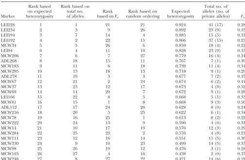
pro-TABLE 1
Values of diversity statistics for each marker and rankings of markers according to the highest number of alleles, highest expected heterozygosity, highest values ofFst, and a random ordering
Rank based Rank based on Total no. of
on expected total no. Rank Rank based on Expected alleles (no. of Marker heterozygosity of alleles based onFst random ordering heterozygosity private alleles) Fst
LEI228 1 1 21 21 0.924 41 (17) 0.281
LEI234 2 3 9 26 0.892 23 (9) 0.334
LEI194 3 7 14 4 0.885 15 (5) 0.314
LEI192 4 2 22 15 0.866 37 (15) 0.255
MCW34 5 5 26 6 0.859 18 (4) 0.228
LEI94 6 4 11 10 0.828 23 (9) 0.330
MCW206 7 6 7 27 0.779 16 (4) 0.341
ADL268 8 18 15 11 0.767 7 (1) 0.309
MCW183 9 11 6 18 0.739 11 (4) 0.346
MCW295 10 13 18 13 0.718 9 (1) 0.295
ADL278 11 19 3 3 0.677 7 (2) 0.376
MCW67 12 21 2 24 0.674 6 (2) 0.417
MCW37 13 23 12 17 0.673 4 (0) 0.320
MCW69 14 14 20 7 0.672 9 (1) 0.282
LEI166 15 22 8 5 0.668 5 (1) 0.337
MCW81 16 15 1 8 0.668 9 (3) 0.501
ADL112 17 17 24 20 0.628 8 (0) 0.247
MCW216 18 20 5 25 0.622 6 (1) 0.347
MCW78 19 16 25 1 0.613 8 (2) 0.228
MCW222 20 24 13 9 0.590 4 (0) 0.315
MCW14 21 10 17 19 0.576 12 (3) 0.297
MCW284 22 25 23 2 0.576 4 (0) 0.254
MCW111 23 12 16 14 0.551 11 (5) 0.303
MCW330 24 9 10 23 0.499 14 (5) 0.331
MCW98 25 26 19 12 0.476 3 (1) 0.287
MCW103 26 27 4 16 0.438 2 (0) 0.373
MCW248 27 8 27 22 0.421 14 (6) 0.189
Ties for the same number of alleles were broken by ranking the average number of alleles per population from largest to smallest.
gram (Felsenstein 1993) to construct the cladogram. We Evaluation of cluster analysis: Each individual was assigned to a specific breed usingstructure (Pritchard et al. 2000), performed 1000 bootstraps across the set of loci to obtain a
consensus cladogram. following the five-step algorithm in Figure 1. In step 1, we chose the value of K, as described above. The aim of the The second approach utilized the programstructure, which
identifies clusters of related individuals from multilocus geno- remaining steps was to assign individuals to breeds and to evaluate the fraction of individuals correctly assigned. In step types (Pritchardet al. 2000). First, we performed many runs
of various lengths with different proposals for the number of 2, we clustered individuals and associated each individual with the cluster that corresponded to the greatest fraction of its genetic clusters (K) represented by the individuals genotyped,
testing all values ofKfrom 1 to 23. Clustering solutions of genome. In step 3, we associated breed labels with each of the inferred genetic clusters. In cases for which a cluster was highest likelihood were obtained when the vast majority of
genomic assignment was distributed over exactly 17, 18, or 19 labeled with multiple breeds, this step required additional subclustering runs ofstructure. These runs used only those clusters. We did not observe clustering solutions in which
⬎19 clusters were assigned nontrivial fractions of the data. To individuals that were assigned to that cluster in step 2, and they lasted 20,000 iterations with a burn-in period of 5000. For choose the best value ofK, we ranstructure20 times for 50,000
steps, after a burn-in period of 5000 steps, using each ofK⫽ subclustering runs,Kequaled the number of breeds associated with the cluster.
17,K⫽18, andK⫽19. Using the Wilcoxon two-sample test,
bothK⫽18 andK⫽19 produced higher likelihood solutions Once the individuals were clustered to the greatest extent possible at the conclusion of step 3, we followed step 4 to assign thanK⫽17 (two-sidedP⫽0.03 forK⫽18vs. K⫽17;
two-sidedP⫽0.04 forK⫽19vs. K⫽17). ForK⫽18 andK⫽ each individual to a single breed. The “clustering success rate” (step 5) was then defined as the proportion of individuals 19, solutions had similar likelihoods (two-sided P ⫽ 0.86).
However, since runs withK⫽19 occasionally produced solu- correctly assigned to their breeds of origin.
Note that we assumed that individuals were maximally clus-tions ofparticularlyhigh likelihood that distributed individuals
over all 19 clusters, 18 was insufficient for maximal clustering, tered after step 3. This assumption avoided additional subclus-tering runs: In principle, a clusterCthat was associated only and we usedK⫽ 19 for all subsequent analyses. Runs used
Figure 1.—Procedure by which cluster analysis was eval-uated. For our data, all breeds had the same number of indi-viduals in the sample. We used
K⫽19,P⫽25,p⫽60.
then be associated with either no breed or with the single minus the proportion of alleles shared by the two individuals. Trees were obtained from distance matrices using theneighbor
breedB. Thus, this subclustering would not greatly affect the
eventual assignment of individuals of clusterCto breeds. We program (Felsenstein1993). If a tree could be partitioned into two connected pieces, each of which contained individu-also did not decompose any subclusters obtained in step 3
into “sub-subclusters.” While it is conceivable that subclusters als from a single breed, the tree was considered “consistent with breed affiliation” (MountainandCavalli-Sforza1997). could be further divided, a single round of subclustering
pro-vided a convenient stopping point for the evaluation, allowing If a tree was consistent with breed affiliation and if the partition of the tree was made by cutting the longest internal edge, the us to devise the precise procedure in Figure 1. Since only a
small number of individuals would have been affected by sub- tree was deemed “strongly consistent with breed affiliation.” If the partition was not necessarily made by cutting this edge, subclustering, the impact of this assumption on the clustering
success rate was likely not very large. In the application of the tree was deemed “weakly consistent with breed affiliation.” For each pair of breeds, we also ran the cluster analysis
structureto data of unknown population structure, however,
subclustering should be performed hierarchically, so that each using 20,000 iterations and a burn-in period of 5000, with
K⫽ 2. The clustering success rate was measured using the cluster, subcluster, or lower-level grouping cannot be further
decomposed. algorithm in Figure 1, though the criterion for subclustering was not met for any pair of populations.
Pairwise cluster analysis:We assessed populations two at a
time with neighbor-joining tree diagrams of the individuals Clustering success as a function of the number of markers: To determine properties of markers that make them effective in in two populations (MountainandCavalli-Sforza1997).
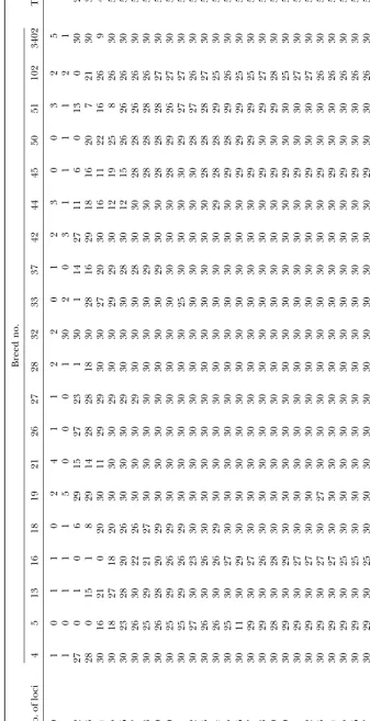
of the original 27 markers according to several variability crite- usually occupied their own clusters, and breeds 18 and ria. For each criterion, and for each value ofM(M⫽1, 2, 3, 37 were often found together in a single cluster. . . . 27), we selected theMmarkers that exhibited the highest
In 9 of the 100 runs performed, 19 clusters were values of that criterion, and we performed cluster analysis
assigned nontrivial fractions of the data. The remaining using that subset of loci. In cases where two or more criteria
produced the same subset, we only performed one analysis for runs included 43, 44, and 4 runs for which 18, 17, and 16 that subset. The criteria included the following: (1) Expected clusters were occupied, respectively. In the 8 solutions of heterozygosity—treating the whole sample as one group, for highest likelihood, breeds 44 and 45 shared a single each locus we computed one minus the sum of the squares
cluster and each of the other 18 breeds occupied an of the sample allele frequencies; (2) total number of alleles
exclusive cluster. The most frequent groupings (Table in the sample—if two or more loci had the same number of
alleles, we broke ties by ranking markers in order of the mean 2), including (5, 16), (16, 18), (18, 37), (33, 44, 45), number of alleles per breed; (3)Fst—we estimatedFstaccording (37, 3402), (42, 50), (44, 45), and (44, 45, 51), appeared toWeir(1996, Equation 5.3). in high-likelihood solutions, while rare groupings were
We also considered marker subsets taken inreverseorder by
obtained in low-likelihood solutions. None of the rare expected heterozygosity, and we used a random ordering of
groupings (13, 26), (16, 33), (21, 26), (26, 42), (28, the loci: For each value of M, we selected the M markers
that were associated with the M highest random numbers. 42), or (33, 51) occurred in any of the 40 solutions of Rankings of markers are shown in Table 1. With the exception highest likelihood. The 10 lowest-likelihood runs con-of orderings induced by the number con-of alleles and expected tained the single instances that produced (21, 26) and heterozygosity (Kendall coefficient⫽0.464,P⫽0.0007), we
(28, 42), as well as three of four instances in which the did not detect evidence for rank correlation among pairs of
grouping (13, 26) was obtained. orderings (of course, the Kendall coefficient was⫺1 for the
orderings by highest and lowest expected heterozygosity, and Breeds that grouped into clusters generally fell close it equaled⫺0.464 for the orderings by highest number of to each other in their placement on the neighbor-join-alleles and lowest expected heterozygosity). ing cladogram (Figure 2), although frequently clustered
Clustering success as a function of the number of individuals:To
groups did not always form clades. Of the eight most see how cluster analysis performed with fewer individuals, for
commonly clustered sets, three did not form clades, each value of N (N ⫽ 5, 10, 15, 20, 25), we repeated the
analysis (with all markers and with marker subsets) usingN namely (33, 44, 45), (16, 18), and (18, 37). Bootstrap randomly chosen individuals from each breed. confidence values for groupings in the cladogram were
generally low.
Pairwise clustering:Although runs using all 20 breeds
RESULTS
clustered pairs or triples of populations because 20 breeds were placed into 19 clusters, cluster analysis using
Genetic differentiation:For each pair of breeds, the
null hypothesis that the two populations had equal allele only the individuals from 2 breeds separated them into 2 clusters. Of 190 pairs, 175 could be perfectly separated frequencies was rejected at the 0.001 significance level
for at least 6 loci (not shown). Even between the most (Table 3). For the remaining 15 pairs, at most 5 individu-als of 60 were placed incorrectly. However, for only 5 closely related pairs of breeds, extremely significant
dif-ferences were found. The only breed pairs for which of these 15 pairs were individuals assigned to the wrong breed with high confidence (⬎75%). The clustering 15 or fewer loci had significantly different allele
frequen-cies at the 0.001 level were (44, 45), (5, 16), (16, 18), success rate was also high for the two triads of popula-tions that grouped together: For both (33, 44, 45) and (18, 26), and (37, 3402). For several pairs, the null
hypothesis of equal allele frequencies was rejected for (44, 45, 51), only individual 45_1 was misplaced (with breed 44).
at least 26 of 27 loci. These pairs included (4, 28), (4,
51), (4, 50), (26, 32), (28, 32), (32, 33), (32, 50), (32, For 188 of 190 breed pairs, the neighbor-joining tree was weakly consistent with breed affiliation (Figure 3). 102), and (37, 102). Genetic distances were generally
large as well (not shown), with only 10 pairwise compari- Of these 188 trees, 170 were strongly consistent with breed affiliation. The 2 pairs for which trees were not sons⬍0.5 and with the average pairwise distance
equal-ing 0.782. The lowest genetic distances were found for consistent (Figure 3), (5, 16) and (44, 45), were among the pairs for which clustering was imperfect. The 18 the following pairs: (44, 45), (5, 16), (16, 18), (18, 37),
and (45, 51). The 25 largest genetic distances involved pairs for which trees were weakly consistent but not strongly consistent with breed affiliation were (5, 18), breeds 4, 19, 32, and 102.
Clustering of breeds: Due to the complexity of the (5, 33), (5, 50), (5, 102), (13, 26), (13, 102), (16, 18),
(16, 50), (16, 102), (18, 37), (27, 102), (28, 102), (33, relationships among the individuals in the data and
the existence of numerous likely clustering solutions, 45), (33, 102), (42, 50), (42, 102), (50, 102), and (51, 102).
different runs ofstructureidentified different potential
clusterings of the individuals (Table 2). Some features Evaluation of clustering: Using the complete set of 27 markers, cluster analysis obtained correct groupings of the clustering were consistent across runs. Most
strik-ingly, breeds 4, 19, 27, 32, and 102 always fell into their of individuals with high accuracy (Figure 4). When only the most polymorphic markers were selected according own clusters, while breeds 44 and 45 always shared the
Figure 2.—Number out of 100 clustering solutions in which multiple breeds occupied the same clusters, superimposed on a neigh-bor-joining cladogram derived from the gen-eralized proportion-of-shared-alleles distance measure. Breed names at branch termini are labeled in boldface type; bootstrap confidence values of breed groupings are italicized next to edges of the cladogram to which they corre-spond; and numbers of clustering solutions are surrounded by brackets inside rectangles enclosing the clusters to which they corre-spond. Bootstrap confidence values are taken over 1000 trees. Rectangles for clustering solu-tions are shown only for groupings that ap-peared in at least 5 of 100 runs. Branch lengths were chosen so that the figure could be conve-niently represented.
heterozygosity, onlyⵑ8–10 markers were needed to at- are highly correlated (in fact, the most variable marker and the set of seven most variable markers coincided tain 95% accurate clusterings. Once 11–12 markers were
chosen, expected heterozygosity, number of alleles, and according to these two criteria) and they produce simi-larly accurate clusterings. However, expected heterozy-Fstperformed similarly, achieving 95–98% in almost
ev-ery run. Although the random ordering achieved 90% gosity is more generally useful—for example, if single nucleotide polymorphisms are used, it provides a natu-clustering accuracy with 10–12 markers, it required
17–20 markers to achieve 95%. The reverse ordering by ral method to rank loci that all have two alleles. Most breeds were clustered perfectly (Table 4), and expected heterozygosity required 14–15 loci to achieve
90% and 17–20 loci to reach 95%. When only a few although clustering solutions differed across runs, the same individuals tended to be misclassified across runs. markers were used, the discrepancy between the two
most effective criteria and the other criteria was ex- For some breeds, including 4, 19, 27, and 32, all individ-uals were perfectly clustered using a small number of tremely high. The marker sets chosen by reverse order of
expected heterozygosity performed particularly poorly highly heterozygous loci. Others, including 5, 13, 16, 18, 44, 45, and 102, required many loci to obtain correct compared to the other methods. However, as the
num-ber of markers increased, all criteria produced nondis- clustering. For breeds 5, 16, 45, and 102, large numbers of markers did not improve classification of a few spe-joint sets of markers, and when nearly all markers were
used, the accuracy of clustering was ⵑ98% for each cific individuals.
When subsets of the individuals were chosen, cluster-criterion.
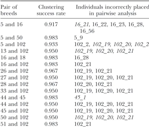
TABLE 3 respond to breed designations. This correspondence essentially holds, although 10–15 individuals frequently Evaluation of cluster analysis in separating pairs of breeds
appeared more similar to breeds from which they did not originate. The inclusion of these individuals in breed Pair of Clustering Individuals incorrectly placed
breeds success rate in pairwise analysis groupings used for the neighbor-joining tree potentially decreases genetic distances of certain pairs and hence 5 and 16 0.917 16_21, 16_22, 16_23, 16_28,
affects the cladogram. However, upon removal of all 16_56
individuals that were sometimes placed incorrectly in 5 and 50 0.983 5_9
pairwise clustering (Table 3), the cladogram was essen-5 and 102 0.933 102_2,102_19,102_20,102_21
13 and 102 0.950 102_19,102_20,102_21 tially unchanged (not shown); thus, these individuals 16 and 18 0.983 16_28 cannot explain its poor reliability.
16 and 102 0.983 102_21 An alternate explanation for the performance of the 26 and 102 0.967 102_19, 102_21 neighbor-joining tree is the fact that in domesticated 27 and 102 0.950 102_19, 102_20, 102_21
species such as chickens, population histories may not 28 and 102 0.967 102_20, 102_21
follow a bifurcating tree model, so that tree diagrams 33 and 102 0.950 102_19, 102_20, 102_21
present a misleading or inaccurate representation of 44 and 45 0.983 45_1
44 and 102 0.950 102_19, 102_20, 102_21 population relationships. The considerable frequency 45 and 102 0.950 102_19, 102_20, 102_21 of gene exchange among historical chicken populations 50 and 102 0.950 102_19,102_20,102_21 could potentially explain the low bootstrap values on
51 and 102 0.983 102_21
internal edges of the tree and on edges that group feral and traditional breeds.
Individuals in italics had at least 75% of their genomes
assigned to the incorrect breed. Fifteen pairs for which cluster- Finally, it is likely thatstructuresimply uses individual ing was imperfect are shown; 175 pairs for which the clustering genotypic data more efficiently than cladograms based success rate was 100% are not shown. Individual identifiers
on genetic distance matrices (Pritchard et al. 2000; include the breed code, an underscore, and the specific
indi-Rosenberget al. 2001). While genetic distance matrices vidual within the breed (for example, 102_20 represents
indi-compress all information about two populations into a vidual 20 in breed 102).
single number, structure does not summarize the data in a unidimensional manner.
90% accuracy (Figure 5). When 10 individuals were It has been argued that 30 markers are insufficient for chosen, 21 markers were sufficient to achieve 90%. distinguishing related populations using phylogenetic When 15 or more individuals were selected from each analysis (Moazami-Goudarzi et al. 1997). With high-breed, 90% accuracy was attained using the 12 most resolution clustering analysis and with careful choices variable loci. of markers, however, far fewer loci sufficed to separate all breeds. The chicken generation interval is short,
ⵑ1 year for these breeds, so that considerable genetic DISCUSSION
variation has built up within and among chicken breeds (Dunningtonet al. 1994;Crooijmanset al. 1996;
Pon-Correspondence of inferred and known population
structure: When the full data set was used, inferred suksiliet al. 1996, 1998, 1999;Mafeniet al. 1997;
Taka-hashi et al. 1998; Vanhala et al. 1998; Hillel et al. genetic clusters of individuals corresponded extremely
well to predefined breed categorizations. Since similar 1999; Wimmers et al. 1999, 2000; Zhou and Lamont 1999;Kaiseret al. 2000). Thus, it is possible that chicken likelihoods of many proposed clusterings make it
diffi-cult to label a “best” clustering of the data, we suggest breeds could be easily separated partly due to high levels of intraspecific variation. However, the success of struc-that, for large data sets, cluster analysis should be
per-formed multiple times before inferences are drawn. All ture when compared to the cladogram in separating breeds makes it likely that the method was largely re-solutions had in common that each cluster contained
all or nearly all individuals from one or a few breeds. sponsible.
In pairwise analysis of populations, clustering and Upon further analysis, all clusters that contained more
than one breed could be subdivided into a collection neighbor-joining trees performed similarly. We note that neighbor-joining trees of individuals from two of subclusters, each of which matched a single breed.
Whilestructure easily separated individuals into clus- breeds are more useful if the strong criterion of separa-tion is used. If genetic origins of individuals in two ters that corresponded almost exactly to phenotypic
labels, the bootstrap neighbor-joining cladogram was populations are known, the weak criterion of consis-tency for separating populations is applicable—two pop-less capable of grouping subsets of the data with great
regularity. Several possibilities can explain this discrep- ulations are separated if there exists a decomposition of the tree into two components, each corresponding to ancy. First, while structure constructs genetic clusters
cor-Figure3.—Neighbor-joining trees of individuals taken from two breeds at a time. (A) One of 170 pairwise neighbor-joining trees that wasstrongly consistent with breed affiliations of individuals. (B) One of 18 neighbor-joining trees that wasweakly
Figure 4.—Clustering suc-cess rate as a function of the number of markers used. Sets of markers were chosen in or-der of five criteria: highest num-ber of alleles, highest expected heterozygosity, lowest expect-ed heterozygosity, highest Fst, and a random ordering.
rate the tree into components; under these circum- private alleles, two or more copies were observed, and, thus, these alleles are unlikely to result from genotyping stances, the strong criterion of consistency must be
ap-plied. When this criterion is used, cluster analysis errors. Since so many alleles in this study were breed specific and since many more were found only in two performs slightly better than neighbor-joining trees in
separating populations. Clustering also offers the oppor- or three breeds, it is possible that these alleles had a substantial effect on clustering success. However, the tunity for significance testing usingR⫻Ctests of
asso-ciation (Rosenberget al. 2001). Permutation tests for number of private alleles in a sample decreases as the sample size from a breed increases. A large number of significance of neighbor-joining clusterings are more
cumbersome. private alleles is not a property of most data sets, and, thus, the highest number of private alleles cannot be
Strategies for successful clustering:Highest expected
heterozygosity and highest number of alleles provided recommended as a criterion method for choosing the best markers to use. In closely related populations, pri-the best ways to select loci for clustering and were better
than highest Fst. This result was surprising: The most vate alleles may be uncommon: for example, using data from a study of 11 human populations (Jinet al. 2000), useful genetic marker for clustering populations and
assigning individuals is one that varies greatly across only 137 of 792 alleles were private to 1 population (and two or more copies were only observed for 41 of these populations but little within them. A perfect locus for
these purposes would be monomorphic within any given 137), even though sample sizes were much smaller than those used here.
breed but polymorphic across breeds (Reed1973). In
the absence of such loci, it seems thatFst, which quanti- The successful performances of all other criteria com-pared to the reverse ordering by expected heterozygos-fies the between-breed component of genetic variation,
should be an appropriate criterion on which to rank ity demonstrate that a careful choice of markers in-creases the power to achieve accurate clustering. This the clustering potential of loci.
Several highly variable markers, the tetranucleotide idea that a careful choice of markers can improve statisti-cal power has been employed in the estimation of popu-loci LEI192 and LEI228 most dramatically, had many
alleles that were specific to at most a few populations lation of origin for admixed individuals (Reed 1973; Shriveret al. 1997). For admixture inference in popula-and frequent in those populations. These markers also
had generally lowFstvalues, since more common alleles tions that result from the combination of two ancestral groups, Shriver et al. (1997) suggested that markers did not greatly differ in frequency across breeds. It
seems likely that these “diagnostic” alleles were partly for assignment should be those with maximal allele fre-quency differentials in the ancestral populations. In the responsible for the extremely successful clustering with
the number of alleles and expected heterozygosity statis- more general situation of a large collection of popula-tions, we suggest that expected heterozygosity, number tics. For 27 markers, we observed 101 alleles private to
Figure 5.—Clustering suc-cess rate as a function of the number of markers and the number of individuals used. The most variable markers were chosen according to the high-est expected heterozygosity in the full data set. Random sets of 5, 10, 15, 20, and 25 individu-als per breed were chosen from among the 30 individuals geno-typed in each breed.
choosing markers for cluster analysis and individual as- done sequentially: A small number of individuals can be genotyped for many markers. The most variable markers signment. All three criteria are applicable to
microsatel-lite data; however, expected heterozygosity is the most can then be selected for future study and then geno-typed in a large sample.
practical general criterion. For some types of markers,
such as single nucleotide polymorphisms, the number While using the most variable markers allows re-searchers to minimize genotyping effort, we caution of alleles is often the same for all markers. The
calcula-tion ofFstpresumes knowledge of population structure, against using this type of marker set with statistical meth-ods that assume a random set of loci and that make so that for initial cluster analysis of a collection of
indi-viduals of unknown origin, the statistic cannot be calcu- inferences based on mean variabilities across loci. A marker set selected for maximal variability will inflate lated. This recommendation of the expected
heterozy-gosity criterion is empirical and potentially of limited estimates of divergence times estimated using the ge-netic distance (␦)2(Goldsteinet al. 1995) and it will generality; the true property of a marker that causes it
to produce successful clusterings is unlikely to be any of bias population growth statistics (e.g.,Zhivotovsky et al. 2000).
the properties mentioned here. A detailed
simulation-based approach will be needed for understanding this We note that the 20 breeds genotyped here were chosen from among many breeds used in an earlier true property.
Depending on the species under consideration, the study (Hillelet al.1999) to maximize diversity within the larger collection of breeds. Thus, it is possible that relative cost of genotyping more individuals and
geno-typing more markers will vary. We did not achieve 90% the populations we used are generally more divergent than populations in other species of interest and even success in clustering when only 5 individuals were used
per breed, but with 10 or more individuals per breed, more divergent than most chicken groups. This is evi-denced by a highFstvalue of 0.313 for these breeds. In clustering was highly successful when enough markers
were used. Similarly, we did not achieve 90% success less diverged populations, including human groups, the number of markers necessary for maximal clustering when fewer than 6–7 markers were used, even when all
individuals were included. Thus, as a minimum, for will certainly be⬎12–15. A more comprehensive analysis
of structure, using simulated data sets of different Fst
similarly diverged populations to those in our study, at
least 12–15 highly variable markers should be genotyped values and different numbers of populations, will be needed to determine the generality of our results. in at least 15–20 individuals per hypothesized
dations. This has allowed us to explore issues that will be used in a training sample for assignment of future be of interest in future applications of genetic cluster unknowns. This training sample can be utilized differ-analysis to data sets of unknown structure, such as the ently by various assignment algorithms. For example, variation of clustering solutions across runs, the differ- the method of Paetkau et al. (1995) estimates allele ence in ease of clustering across populations, and the frequencies from a training sample and assigns each placement of problematic individuals. unknown individual to the population in which its
geno-Problematic individuals:In most runs, the clustering type is most likely, assuming Hardy-Weinberg and
link-success rate remained⬍ⵑ98%, though this level could age equilibrium. The method ofCornuetet al.(1999) be obtained when 15–20 highly variable markers were also estimates population allele frequencies from a train-used. Given this observation, it is surprising that the full ing sample and uses the smallest genetic distance of set of 27 markers did not achieve 100% accuracy. Errors the unknown individual to the various populations for in the clustering algorithm seem to be an unlikely expla- assignment. With thestructurealgorithm ofPritchard nation, since roughly the same sets of individuals were et al.(2000), a genetic clustering solution is obtained placed in the wrong clusters in runs that used different that includes the training sample and the unknowns. sets of loci or that produced different clustering solu- Next, each unknown is assigned to a cluster. Finally, tions. Since all breeds were sampled from populations depending on which individuals from the training sam-maintained in different locations, it is unlikely that re- ple are also assigned to that cluster, the unknown is cent admixture or labeling errors explain the improper eventually assigned to a breed. During this process, prior placements. We suspect that the inability to achieve knowledge about individuals in the training sample can perfect clustering results from the fact that some individ- be incorporated—individuals in the training sample can uals were genetically atypical of their breeds, and the be flexibly treated as being of known, unknown, or algorithm could not recognize breeds of origin for these probabilistically known origin.
individuals. The frequently misplaced individuals 102_19, The importance of training samples for population 102_20, and 102_21 derived from a flock of zoo animals assignment suggests a strategy by which future assign-that may have undergone considerable genetic drift. ment studies can be optimized. For any species of inter-Individuals 16_21, 16_22, and 16_23 came from a single est, the most variable markers according to expected flock, one of many that was incorporated into the breed heterozygosity, number of alleles, or
Fstshould be geno-16 sample; this flock may have been managed differently
typed on a large scale. New markers could be tested by from the others. Interestingly, only one individual was
the criterion, and highly variable new markers could misplaced from the closely related breeds 44 and 45:
potentially be included in the set of most variable mark-This suggests thatstructuremay be useful for
distinguish-ers, reducing the number of markers needed for cluster-ing lines from different breedcluster-ing companies, in spite
ing studies below the current recommendation of 12– of common origin and similar selection objectives.
15. A database of individual genotypes at these most
Cluster analysis and population assignment:
Place-variable loci could then be made publicly available. New ment of individuals into clusters is related, but not
iden-individuals could be genotyped for the most variable tical, to assignment of unknown individuals to
popula-markers and could then be added to the database. Indi-tions. Assignment tests assume the existence of distinct
viduals in the database who are known to represent populations and use properties of those groups, such
certain breeds could be used as a training sample for as allele frequencies, to infer the source populations of
assignment tests. Individuals who were misassigned or unknown individuals (Buchananet al. 1994;Paetkau
who were difficult to assign correctly could be excluded
et al. 1995;RannalaandMountain1997;Cornuetet
from the database, so that only the individuals who can
al. 1999; Davies et al. 1999; Ciampolini et al. 2000;
confidently be assigned to the correct breeds would be Pritchard et al. 2000). Properties of the potential
included. source populations are ideally known, but in practice
Such a database might be extremely useful to re-they are generally inferred in such a way that any specific
searchers who may only have one or a few unknown indi-individual is not assigned using information that derived
viduals that they wish to identify (e.g., Primmer et al. from knowledge of its genotype. In our evaluation
pro-2000). This type of database could also serve as a reposi-cedure, individuals are first used to create clusters, and
tory of individuals with known origin for testing new the same individuals are assigned to clusters and then
statistical algorithms. Using such a database, genetic to breeds. While this approach allows us to precisely
variation quantified in different studies can be made define the clustering success rate, the fact that
informa-commensurable, and large numbers of individual multilo-tion from any given individual is used in inferring its
cus genotypes can be combined into a single framework. origin prevents us from interpreting its inferred
popula-The importance of training samples to assignment tion of origin as a proper assignment.
makes it necessary that the same microsatellite allele Our results are best interpreted as verification that
sizes be used by different laboratories. DNA from several these individuals indeed form genetic clusters that
Tixier-Boichard to calibrate allele size measurements, and ge- ulations (42 and 50), as well as other collections of populations that were of the same general category. The notypes are available at http://charles.stanford.edu.
Cluster analysis and genetic distinctiveness: We ob- combinations (33, 44, 45), (37, 3402), and (44, 45, 51)
all included selected populations. The grouping (18, served that some breeds were easier to separate into
clusters than others, in the sense that all individuals in 37) may reflect the fact that breeds 18 and 37 are unse-lected and seunse-lected descendants, respectively, of ances-some breeds were correctly placed with only a small
number of markers. This likely derives from the pres- tral white leghorn populations. Groupings of traditional breeds, such as (5, 16) and (16, 18), are more surprising. ence of distinctive multilocus genetic combinations in
the breeds that were easiest to separate. Thus, we suggest It seems particularly strange that the Icelandic landrace (16), probably isolated for several hundred years, would that the relative number of loci required for the correct
clustering of several breeds can be used as a way of sometimes group with the Middle Eastern Bedouin breed (5). One hypothesis is that populations 5, 16, identifying populations that are genetically distinctive
with respect to a collection. and 18 represent unselected groups similar to ancestral Mediterranean chickens, which may have colonized In addition to resolving questions about population
histories (Rosenberg et al. 2001), the characterization many European countries along maritime trading routes. A more detailed historical analysis of chicken of genetically distinctive populations can assist in
conser-vation of within-species diversity (Moritz1994;Paet- breeds will be required to explain such surprising rela-tionships.
kau 1999). For species in which relative conservation
value of different populations is of interest, the ease Conclusions:We have discussed the application of gene-tic cluster analysis to 600 individuals from 20 chicken with which a population can be separated from other
groups by cluster analysis can be incorporated into as- breeds, demonstrating that the technique has great po-tential to correctly identify population structure. We sessments of its conservation potential, along with
rele-vant ecological, economic, and evolutionary criteria. have argued that individual clustering provides a more appropriate characterization of population structure in More generally, cluster analysis has great potential to
help identify populations with different allele frequen- these groups than does a neighbor-joining tree. Last, we have proposed recommendations on future uses of cies and different multilocus genetic combinations.
Al-though genetical divergence among populations may genetic cluster analysis and individual assignment tests in similarly diverged collections of populations: (1) At not reflect adaptive diversity (Crandall et al. 2000),
conservation programs that wish to maintain genetic least 12–15 highly variable loci should be genotyped in at least 15–20 individuals per hypothesized population; diversity of endangered species could benefit from a
purely genetical method by which individuals can be (2) markers with the highest expected heterozygosity, number of alleles, andFstcan be used in genetic cluster clustered without regard to their sampling location. For
agricultural species, although the preservation of spe- analysis to minimize genotyping costs; (3) databases of multilocus genotypes obtained at highly variable mark-cific phenotypes is perhaps of primary interest,
conser-vation of genetic diversity is of great importance toward ers in individuals of known origins can be established to provide training samples for assignment algorithms; ensuring that future breeding programs will have a large
base on which to perform artificial selection (Notter (4) genetically distinctive populations can be identified on the basis of how difficult it is to separate them from 1999).
Relationships of chicken breeds:Considerable atten- other breeds when cluster analysis is used; and (5)
clus-ter analysis can provide an additional tool for identifica-tion has been devoted to the study of genetic diversity
and relationships of chickens. Some studies focused on tion of population relationships, history, and within-species genetic units for conservation.
commercial breeds (Dunningtonet al. 1994;
Crooij-manset al. 1996;Kaiseret al. 2000), others mainly con- The authors thank Nina Dudnik and Jonathan Pritchard for helpful
sidered local breeds (Mafeniet al. 1997;Takahashiet comments. This study arose during a visit by N.A.R. to the laboratory of J.H. N.A.R. is supported by a Program in Mathematics and Molecular
al. 1998;Wimmerset al. 1999, 2000), and some studied
Biology graduate fellowship. This research was supported by the
Euro-mixed collections (Ponsuksiliet al. 1996, 1998, 1999;
pean Community-funded project AVIANDIV (Development of Strat-Vanhala et al. 1998; Hillel et al. 1999; Zhou and
egy and Application of Molecular Tools to Assess Biodiversity in Lamont1999). We suggest here that the frequent clus- Chicken Genetic Resources, BIO4CT980342) and by National Insti-tering of pairs of breeds into the same clusters illumi- tutes of Health grant GM28428 to M.W.F.
nates a new approach toward determining genetic simi-larity. Populations can be considered similar if they are
frequently placed in the same genetic cluster. Several LITERATURE CITED
of the frequently obtained groupings of populations Beaumont, M., E. M. Barratt, D. Gottelli, A. C. Kitchener, M. J. Danielset al., 2001 Genetic diversity and introgression in the
are expected from knowledge of chicken population
Scottish wildcat. Mol. Ecol.10:319–336.
histories. The two most difficult populations to separate
Bowcock, A. M., A.Ruiz Linares, J.Tomfohrde, E.Minch, J. R.
were the two commercial brown-egg layers (44 and 45). Kiddet al., 1994 High resolution of human evolutionary trees
with polymorphic microsatellites. Nature368:455–457.
pop-Buchanan, F. C., L. J. Adams, R. P. Littlejohn, J. F. Maddoxand tion units: a critique of current methods. Conserv. Biol.13:1507– 1509.
A. M. Crawford, 1994 Determination of evolutionary
relation-Paetkau, D., W. Calvert, I. StirlingandC. Strobeck, 1995 Mi-ships among sheep breeds using microsatellites. Genomics22:
crosatellite analysis of population structure in Canadian polar 397–403.
bears. Mol. Ecol.4:347–354.
Ciampolini, R., H. Leveziel, E. Mazzani, C. GrohsandD. Cianci,
Ponsuksili, S., K. WimmersandP. Horst, 1996 Genetic variability 2000 Genomic identification of the breed of an individual or
in chickens using polymorphic microsatellite markers. Thai J. its tissue. Meat Sci.54:35–40.
Agric. Sci.29:571–580.
Cornuet, J.-M., S. Piry, G. Luikart, A. EstoupandM. Solignac,
Ponsuksili, S., K. WimmersandP. Horst, 1998 Evaluation of ge-1999 New methods employing multilocus genotypes to select
netic variation within and between different chicken lines by or exclude populations as origins of individuals. Genetics153:
DNA fingerprinting. J. Hered.89:17–23. 1989–2000.
Ponsuksili, S., K. Wimmers, F. Schmoll, P. HorstandK. Schel-Crandall, K. A., O. R. P. Bininda-Emonds, G. M. MaceandR. K.
lander, 1999 Comparison of multilocus DNA fingerprints and
Wayne, 2000 Considering evolutionary processes in
conserva-microsatellites in an estimate of genetic distance in chicken. J. tion biology. Trends Ecol. Evol.15:290–295.
Hered.90:656–659.
Crooijmans, R. P. M. A., A. F. Groen, A. J. A. Van Kampen, S.
Primmer, C. R., M. T. KoskinenandJ. Piironen, 2000 The one
Van Der Beek, J. J. Van Der Poelet al., 1996 Microsatellite
that did not get away: individual assignment using microsatellite polymorphism in commercial broiler and layer lines estimated data detects a case of fishing competition fraud. Proc. R. Soc. using pooled blood samples. Poult. Sci.75:904–909. Lond. Ser. B267:1699–1704.
Davies, N., F. X. VillablancaandG. K. Roderick, 1999 Determin- Pritchard, J. K., M. StephensandP. J. Donnelly, 2000 Inference ing the source of individuals: multilocus genotyping in nonequi- of population structure using multilocus genotype data. Genetics librium population genetics. Trends Ecol. Evol.14:17–21. 155:945–959.
Devlin, B., andK. Roeder, 1999 Genomic control for association Rannala, B., andJ. L. Mountain, 1997 Detecting immigration by studies. Biometrics55:997–1004. using multilocus genotypes. Proc. Natl. Acad. Sci. USA94:9197–
Dunnington, E. A., L. C. Stallard, J. Hilleland P. B. Siegel, 9201.
1994 Genetic diversity among commercial chicken populations Reed, T. E., 1973 Number of gene loci required for accurate estima-estimated from DNA fingerprints. Poult. Sci.73:1218–1225. tion of ancestral population proportions in individual human
Felsenstein, J., 1993 PHYLIP (Phylogeny Inference Package).Depart- hybrids. Nature244:575–576.
Rosenberg, N. A., E. Woolf, J. K. Pritchard, T. Schaap, D. Gefel
ment of Genetics, University of Washington, Seattle.
et al., 2001 Distinctive genetic signatures in the Libyan Jews.
Goldstein, D. B., A. Ruiz Linares, L. L. Cavalli-SforzaandM. W.
Proc. Natl. Acad. Sci. USA98:858–863.
Feldman, 1995 Genetic absolute dating based on
microsatel-Saitou, N., andM. Nei, 1987 The neighbor-joining method: a new lites and the origin of modern humans. Proc. Natl. Acad. Sci.
method for reconstructing phylogenetic trees. Mol. Biol. Evol. USA92:6723–6727.
4:406–425.
Groenen, M. A. M., H. H. Cheng, N. Bumstead, B. F. Benkel, W. E.
Shriver, M. D., M. W.Smith, L.Jin, A.Marcini, J. M.Akeyet al.,
Briles et al., 2000 A consensus linkage map of the chicken
1997 Ethnic-affiliation estimation by use of population-specific genome. Genome Res.10:137–147.
DNA markers. Am. J. Hum. Genet.60:957–964.
Hillel, J., A. Korol, V. Kirzner, P. Freidlin, S. Weigendet al., 1999
Takahashi, H., K. Nirasawa, Y. Nagamine, M. TsudzukiandY.
Biodiversity of chickens based on DNA pools: first results of the
Yamamoto, 1998 Genetic relationships among Japanese native EC funded project AVIANDIV, pp. 22–29 inPoultry Genetics
Sympo-breeds of chicken based on microsatellite DNA polymorphisms.
sium,Proceedings, edited by R.Preisinger. Lohmann Tierzucht, J. Hered.89:543–546.
Cuxhaven, Germany. Tixier-Boichard, M., G. CoquerelleandC. Vilela-Lamego, 1999
Jin, L., M. L. Baskett, L. L. Cavalli-Sforza, L. A. Zhivotovsky, Contribution of data on history, management and phenotype M. W. Feldmanet al., 2000 Microsatellite evolution in modern to the description of the diversity between chicken populations humans: a comparison of two data sets from the same populations. sampled within the AVIANDIV project, pp. 15–21 inPoultry
Genet-Ann. Hum. Genet.64:117–134. ics Symposium, Proceedings, edited by R. Preisinger. Lohmann
Kaiser, M. G., N. Yonash, A. CahanerandS. J. Lamont, 2000 Mi- Tierzucht, Cuxhaven, Germany.
crosatellite polymorphism between and within broiler popula- Vanhala, T., M. Tuiskula-Haavisto, K. Elo, J. VilkkiandA. Ma¨ki
-tions. Poult. Sci.79:626–628. Tanila, 1998 Evaluation of genetic variability and genetic
dis-Mafeni, M. J., K. WimmersandP. Horst, 1997 Genetic diversity tances between eight chicken lines using microsatellite markers. in indigenous Cameroon and German Dahlem Red fowl popula- Poult. Sci.77:783–790.
Weigend, S., 1999 Assessment of biodiversity in poultry with DNA tions estimated from DNA fingerprints. Arch. Tierz.40:581–589.
markers, pp. 7–14 inPoultry Genetics Symposium,Proceedings, edited
Minch, E., A. Ruiz-Linares, D. B. Goldstein, M. W. Feldmanand
by R.Preisinger. Lohmann Tierzucht, Cuxhaven, Germany.
L. L. Cavalli-Sforza, 1998 Microsat2: A Computer Program for
Weir, B. S., 1996 Genetic Data Analysis II. Sinauer Associates,
Sunder-Calculating Various Statistics on Microsatellite Allele Data. Department
land, MA. of Genetics, Stanford University, Stanford, CA.
Wimmers, K., S. Ponsuksili, F. Schmoll, T. Hardge, E. B. Sonaiyaet
Moazami-Goudarzi, K., D. Laloe¨, J. P. FuretandF. Grosclaude,
al., 1999 Application of microsatellite analysis to group chicken 1997 Analysis of genetic relationships between 10 cattle breeds
according to their genetic similarity. Arch. Tierz.42:629–639. with 17 microsatellites. Anim. Genet.28:338–345.
Wimmers, K., S. Ponsuksili, T. Hardge, A. Valle-Zarate, P. K. Moritz, C., 1994 Defining ‘evolutionarily significant units’ for
con-Mathuret al., 2000 Genetic distinctness of African, Asian and servation. Trends Ecol. Evol.9:373–375.
South American local chickens. Anim. Genet.31:159–165.
Mountain, J., andL. L. Cavalli-Sforza, 1997 Multilocus
geno-Zhivotovsky, L. A., L. Bennett, A. M. BowcockandM. W. Feldman, types, a tree of individuals, and human evolutionary history. Am.
2000 Human population expansion and microsatellite
varia-J. Hum. Genet.61:705–718. tion. Mol. Biol. Evol.17:757–767.
National Research Council, 1996 The Evaluation of Forensic DNA Zhou, H., andS. J. Lamont, 1999 Genetic characterization of biodiv-Evidence. National Academy Press, Washington, DC. ersity in highly inbred chicken lines by microsatellite markers.
Notter, D. R., 1999 The importance of genetic diversity in livestock Anim. Genet.30:256–264. populations of the future. J. Anim. Sci.77:61–69.