A New Thermal Conductivity Model for Nanofluids with Convection Heat Transfer Application

ABSTRACT

YU, FENG. A New Thermal Conductivity Model for Nanofluids with Convection Heat Transfer Application. (Under the direction of Dr. C. Kleinstreuer).

A nanofluid is a dilute suspension of nanometer-sized particles and fibers dispersed in a liquid. As a result, when compared to the base fluid, alteration of physical properties of mixtures occurs, such as viscosity, density and thermal conductivity, among others. Of all the physical properties of nanofluids, the thermal conductivity is the most complex and important one. Interestingly, experimental findings have been controversial and theories did not fully explain the phenomenon of elevated thermal conductivity. Hence, a new theory based on first principles is needed to describe the mechanisms of the anomalous enhancement on thermal conductivity of nanofluids.

Such a new theory, i.e., the Feng-Kleinstreuer (F-K) model, is derived in Chapter 2 relying on basic physics and fluid dynamics aspects, where a statistical method was used to take the particle-particle interaction into account, the Reynolds-averaged heat transfer equation was solved, the fluctuation velocity was treated as a function of the distance between particle and “fluid package”, and the induced fluctuation velocities were superimposed to implement multi-particle effects. More specifically, the new thermal conductivity expression consists of a base-fluid static part, kbf, and a new “micro-mixing”

part, kmm, so that knf = kbf + kmm. While kbf relies on Maxwell’s theory, kmm encapsulates

extended Langevin equation with scaled interaction forces, and a turbulence-inspired heat transfer equation.

Comparisons between the F-K model and benchmark experimental data sets as well as other theories were successfully carried out, focusing mainly on alumina and copper-oxide nanoparticles (20<dp<50nm) in water with volume fractions up to 5% and mixture

temperature below 350K. The new theory can be readily extended to accommodate other forms of nanoparticle-liquid pairings and to include non-spherical nanomaterial.

Based on the potentially significant enhancement in thermal conductivity, nanofluids are expected to be suitable for practical cooling applications with little or no penalty in pressure drop. While the conventional convective heat transfer correlations for pure fluids are not suitable for nanofluids, research on the convective heat transfer properties of nanofluids is necessary. It should not only focus on the Nusselt number (Nunf) and heat transfer coefficient

(hnf), but also on the friction factor, pressure drop and effective viscosity of nanofluids.

Clearly, the convective heat transfer properties depend not only on the thermal conductivity but on other properties as well, such as the specific heat, density, and dynamic viscosity of fluids.

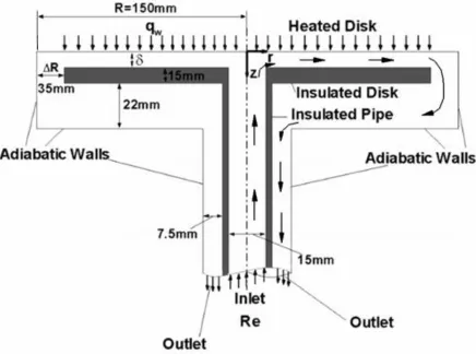
As a representative application, nanofluid flow between parallel disks of an impinging jet is investigated in Chapter 3. It focuses on the improvement performance in cooling by using nanofluids, with the new Feng-Kleinstreuer model for the thermal conductivity. Nusselt number Nunf, heat transfer coefficient hnf, friction factor fD, and pressure p were investigated

A New Thermal Conductivity Model for Nanofluids with Convection Heat Transfer Application

by Yu Feng

A thesis submitted to the Graduate Faculty of North Carolina State University

in partial fulfillment of the requirements for the degree of

Master of Science

Mechanical Engineering

Raleigh, North Carolina 2010

APPROVED BY:

________________________________ ______________________________ Dr. C. Kleinstreuer Dr. S. Lubkin

Committee Chair

________________________________ ______________________________ Dr. T. Ward Dr. Y. Zhu

ii

DEDICATION

iii

BIOGRAPHY

The author was born on September 8, 1984 in Shenyang, Liaoning Prov., China

After graduating from Northeast Yucai high school, he was admitted to Zhejiang University (ZJU) in 2003 and studied in the Department of Mechanics and earned his Bachelor of Science degree in 2007. He continued 1 year graduate study in the same department concentrating on Brownian coagulation of aerosol particles.

Afterwards, the author enrolled as a doctoral student August, 2009 in the Department of Mechanical and Aerospace Engineering at North Carolina State University in Raleigh, NC. His MS dissertation research focused on nanofluid heat transfer properties analysis and computational nanofluid flow in micro-systems. He is being supported by the China Scholarship Council (CSC) and partially by a grant from the National Science Foundation (NSF).

iv

ACKNOWLEDGMENTS

I would like to express a great deal of appreciation for Dr. C. Kleinstreuer, Chairman of my advisory committee. His physical insight, guidance and encouragement have been the impetus for me to keep working hard and to succeed. He has proven to be a very considerate and patient advisor who serves as a role model for professional excellence and integrity. It is he who provided me with the research direction that I dreamed to focus on. He gave me confidence at the time when I was confused for my future academic directions; He who demonstrated to me that it is more amazing on the way to the destination of research than the destination.

I would like to express the greatest gratitude to my mother country, China. Without the fellowship from the China Scholarship Council, I could not even have dreamed of coming to the United States to pursue the degree.

v members in our Computation Fluid-Particle Dynamics Laboratory, including Dr. Z. Zhang, and Miss E. Childress.

vi

TABLE OF CONTENTS

LIST OF TABLES ... ix

LIST OF FIGURES ... x

CHAPTER 1 INTRODUCTION and LITERATURE REVIEW ... 1

1.1 Introduction ...2

1.2 Motivation ...4

1.3 Research Objectives ...6

1.4 Nanofluid Conduction Heat Transfer Properties ...7

1.4.1 Experimental Methods and Observations ...7

1.4.2 Numerical Methods and Observations ...16

1.4.3 Theoretical Models ...20

1.5 Nanofluid Convective Heat Transfer Properties ...26

1.5.1 Heat transfer coefficient (hnf) and Nusselt number (Nu) ...27

1.5.2 Viscosity of Nanofluids ...30

1.5.3 Friction factor (fnf) and pressure drop ...34

1.6 Impinging Jet Cooling Systems ...37

1.6.1 Impinging Jets Applications ...37

1.6.2 Convective Heat Transfer Properties of Impinging Jets ...38

CHAPTER 2 A NEW THERMAL CONDUCTIVITY MODEL for NANOFLUID FLOW ...51

2.1 Introduction ...52

2.2 Parameter Decomposition ...54

2.3 Mechanisms ...55

2.3.1 Base Fluid-Particle Interaction ...56

2.3.2 Forces acting on Nanoparticle ...60

vii

2.3.4 Base Fluid-Base Fluid Interaction ...64

2.4 Relative-Order-of-Magnitude Analysis for Forces ...64

2.5 Governing Equations ...65

2.6 Reduced Governing Equations ...67

2.6.1 Energy Equation...67

2.6.2 Extended Langevin Equation ...68

2.6.3 Relationship between T’ and T ...70

2.7 Thermal Conductivity of Nanofluids ...71

2.7.1 Expression for kmm ...72

2.7.2 Expression for knf ...74

2.7.3 Dependencies of Parameters in New Model ...75

2.8 Comparisons ...78

2.8.1 Comparisons with Benchmark Experimental Data ...78

2.8.2 Comparisons with other Theoretical Models ...82

2.9 Summary ...87

CHAPTER 3 NANOFLUID FLOW APPLICATION...105

3.1 Introduction ...106

3.2 Theory ...108

3.2.1 Governing Equations ...108

3.2.2 Reduced Governing Equations ...111

3.2.3 Analytical Velocity Solution for Reduced Governing Equations ...113

3.3 Model Validations ...115

3.3.1 Numerical Methods ...115

3.3.2 Velocity Field Validations ...116

3.3.3 Temperature Field Validations ...119

3.4 Results and Discussion ...121

3.4.1 Flow Structures ...121

viii

3.4.3 Convective Heat Transfer Analysis ...127

3.4.4 Entropy Generation Analysis ...140

3.5 Maximum Wall Temperature Control ...149

3.6 Conclusions ...151

CHAPTER 4 CONCLUSIONS and FUTURE WORK ...205

4.1 Conclusions and Novel Contributions ...206

4.2 Future Work ...208

ix

LIST OF TABLES

Table 1.1 Thermal Conductivities of Different Materials ...48 Table 1.2 Classical Models for Effective Thermal Conductivity of Mixtures ...49 Table 1.3 Summary of Experimental Studies on Convective

x

LIST OF FIGURES

Fig. 1.1 Thermal conductivity ranges for different materials ...40

Fig. 1.2 (a) Sketch of a typical transient hot wire measurement device ...41

Fig. 1.2 (b) Wheatstone bridge circuit for transient hot-wire method ...42

Fig. 1.2 (c) Photos of a real transient hot-wire device ...42

Fig. 1.3 Sketch and photo experimental device of thermal-lensing measurement method ...43

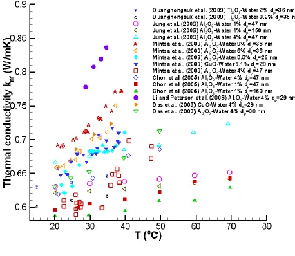
Fig. 1.4 Benchmark and newly published experimental data of nanofluids thermal conductivity as a function of temperature T ...44

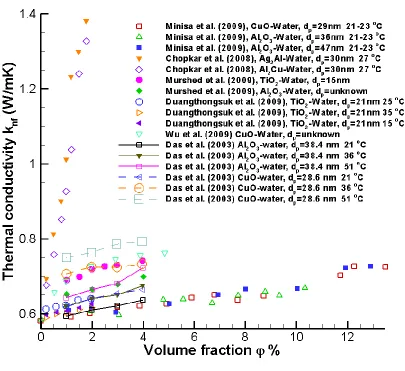
Fig. 1.5 Benchmark and newly published experimental data of nanofluids thermal conductivity as a function of particle volume fraction φ ...45

Fig. 1.6 (a) Mesh details for numerical simulation by Li and Peterson (2007) ...46

Fig. 1.6 (b) Temperature contour around nanoparticles ...46

Fig. 1.7 A typical experimental setup to measure convective heat transfer properties ...47

Fig. 2.1 Sketch for multi-nanoparticle Brownian motion influence on base fluid ...89

Fig. 2.2 Sketch for capturing sphere around fluid package ...90

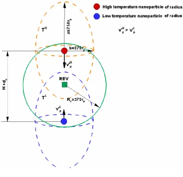
Fig. 2.3 Sketch for induced velocities due to nanoparticles in different temperatures ...91

Fig. 2.4 Spherical coordinates and Cartesian coordinates for calculating Stokes flow around a particle ...92

Fig. 2.5 F-K model predictions for nanofluids dependence on temperature ...93

Fig. 2.6 Comparisons between F-K model and benchmark experimental data for Al2O3-water nanofluids dependence on volume fraction φ ...94

Fig. 2.7 Comparisons between F-K model and benchmark experimental data for Al2O3-water nanofluids dependence on volume fraction T ...95

xi

CuO-water nanofluids dependence on volume fraction φ ...96

Fig. 2.9 Comparisons between F-K model and benchmark experimental data for ZrO2-water and TiO2-water nanofluids dependence on volume fraction φ ...97

Fig. 2.10 Comparison between F-K model and Cu-water nanofluid experimental data ...98

Fig. 2.11 Comparison between F-K model with revised Kp-p and Cu-water nanofluid experimental data ...99

Fig. 2.12 Comparisons between F-K model and MSB model ...100

Fig. 2.13 Comparisons between F-K model and Bao’s model ...101

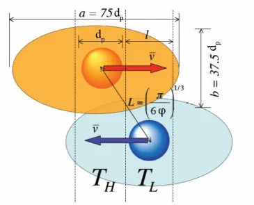
Fig. 2.14 Illustrative sketch explaining the particles’ Brownian-motion effect on micro-mixing for Koo-Kleinstreuer model ...102

Fig. 2.15 Comparisons between KKL model and benchmark experimental data ...103

Fig. 3.1 Sketch of the radial flow cooling system...152

Fig. 3.2 Sketch of multi-impinging jet cooling system ...153

Fig. 3.3 Example of impinging jet cooling system used in chip cooling ...154

Fig. 3.4 Simplified model of the cooling system ...155

Fig. 3.5 Mesh details for the cooling system ...156

Fig. 3.6 Velocity profiles comparison between numerical solution and simplified theoretical solution for δ=3mm...157

Fig. 3.7 Velocity profiles comparison between numerical solution and simplified theoretical solution for δ=2mm...158

Fig. 3.8 Velocity contour at plane θ=π/4 for 4% Al2O3-water nanofluid with Renfin=500...159

Fig. 3.9 (a) Velocity field near the corner at r=0 (Maiga, 2005) ...160

Fig. 3.9 (b) Velocity field near the corner at r=0 (Roy, 2004) ...160

xii and experimental data ...162 Fig. 3.12 Wall temperature and bulk temperature along r-direction for 2%

Al2O3-water nanofluid with Re=500 ...163

Fig. 3.13 Velocity profile development for δ=2mm 4% Al2O3-water nanofluid

with Re=333.33 ...164 Fig. 3.14 (a)-(c) Velocity contours comparison for cooling system δ=2mm with different inlet Reynolds numbers (a) Renfin=150 (b) Renfin=300 (c) Renfin=500 ...165

Fig. 3.14 (d)-(f) Temperature contours comparison for cooling system δ=2mm with different inlet Reynolds numbers (d) Renfin=150 (e) Renfin=300 (f) Renfin=500 ...166

Fig. 3.15 (a) Flow structure for flow between parallel disks with δ=3mm...167 Fig. 3.15 (b) Flow structure for flow between parallel disks with δ=2mm ...167 Fig. 3.16 Temperature profiles development between two parallel disks along

the r-direction for 4% Al2O3-water nanofluid ...168

Fig. 3.17 (a) Temperature contour for 4% Al2O3-water nanofluid with Renfin=500

and artificial knf=0.9625 W/mK ...169

Fig. 3.17 (b) Temperature contour for 4% Al2O3-water nanofluid between parallel

disks with qw=2438 W/m2 and mass flow rate 0.019kg/s ...169

Fig. 3.18 Wall temperatures comparison between Re=200 and Re=500 for 4%

Al2O3-water nanofluid ...170

Fig. 3.19 Comparison of wall temperatures and bulk temperatures between two parallel disks along the r-direction for 4% Al2O3-water nanofluid with δ=2mm

and δ=3mm ...171 Fig. 3.20 Wall temperature comparisons between nanofluids with different particle

diameter...172 Fig. 3.21 Wall temperature comparison between 4% dp=47nm Al2O3-water nanofluid

and pure water ...173 Fig. 3.22 Wall temperature comparison between 2%, 4% dp=38.4nm Al2O3-water

xiii Fig. 3.23 (a) Temperature contour for pure water with δ=2mm ...175 Fig. 3.23 (b) Temperature contour for 2% Al2O3-water nanofluid with δ=2mm ...175

Fig. 3.23 (c) Temperature contour for 4% Al2O3-water nanofluid with δ=2mm ...175

Fig. 3.24 Heat transfer coefficient hnf comparison between nanofluids with different

particle diameter...176 Fig. 3.25 Nusselt number Nunf comparison between nanofluids with different

particle diameter...177 Fig. 3.26 Heat transfer coefficient hnf comparison between nanofluids with different

particle volume fraction ...178 Fig. 3.27 Nusselt number Nunf comparison between nanofluids with different

particle volume fraction ...179 Fig. 3.28 Heat transfer coefficient hnf comparison between pure water and 4%

dp=47nm Al2O3-water nanofluid ...180

Fig. 3.29 Nusselt number Nunf comparison between pure water and 4%

dp=47nm Al2O3-water nanofluid ...181

Fig. 3.30 Heat transfer coefficient hnf comparison between 4% dp=47nm Al2O3-water

nanofluids with different inlet Reynolds numbers ...182 Fig. 3.31 Nusselt number Nunf comparison between 4% dp=47nm Al2O3-water

nanofluids with different inlet Reynolds numbers ...183 Fig. 3.32 Relationship between Nusselt number and Brinkman number

with different disk-spacing for different Reynolds numbers and at qw=20kW/m2 ...184

Fig. 3.33 Free body diagram of REV for pressure drop analysis ...185 Fig. 3.34 Friction factors along r-direction for 4% dp=47nm Al2O3-water nanofluids

with different inlet Reynolds numbers ...186 Fig. 3.35 Friction factor comparisons between theoretical prediction and

xiv numerical simulations for nanofluids with different inlet temperatures ...188 Fig. 3.37 Friction factor comparisons between correlated theoretical prediction and

numerical simulations for nanofluids with different inlet temperatures ...189 Fig. 3.38Pressure comparisons along r-direction between theoretical

predictions and numerical simulations for 4% dp=47nm Al2O3-water nanofluids

with different inlet Reynolds numbers ...190 Fig. 3.39 Pressure comparisons along r-direction between theoretical

predictions and numerical simulations for 4% dp=38.4nm Al2O3-water nanofluids ...191

Fig. 3.40Pressure comparisons along r-direction between theoretical

predictions and numerical simulations for dp=38.4nm Al2O3-water nanofluids

with different volume fractions ...192 Fig. 3.41 Frictional entropy generation rate per unit volume comparisons

between theoretical predictions and numerical simulations at upper and lower disks ....193 Fig. 3.42 Frictional entropy generation rate per unit volume comparisons

between theoretical predictions and numerical simulations at axial plane ...194 Fig. 3.43 (a) Frictional entropy generation rate per unit volume contours for

nanofluids with Tin=297K ...195

Fig. 3.43 (b) Frictional entropy generation rate per unit volume contours for

nanofluids with Tin=308K ...195

Fig. 3.44 (a) Heat transfer entropy generation rate per unit volume contours for

nanofluids with Tin=297K ...196

Fig. 3.44 (b) Heat transfer entropy generation rate per unit volume contours for

nanofluids with Tin=308K ...196

Fig. 3.45 (Tw-Tin) along r-direction for nanofluids with different inlet temperatures…..197

Fig. 3.46 Heat transfer and frictional entropy generation rate for 4% dp=47nm

Al2O3-water nanofluids with different inlet Temperature ...198

Fig. 3.47 (a) Heat transfer entropy generation rate per unit volume contours for

xv Fig. 3.47 (b) Heat transfer entropy generation rate per unit volume contours for

nanofluids with φ=2% ...199 Fig. 3.47 (c) Heat transfer entropy generation rate per unit volume contours for

nanofluids with φ=4% ...199 Fig. 3.48Entropy generation rate for Al2O3-water nanofluids with different

nanoparticle volume fractions ...200 Fig. 3.49 Heat transfer entropy generation rate for 4% dp=47nm Al2O3-water

nanofluids with different inlet Reynolds numbers ...201 Fig. 3.50 Frictional entropy generation rate for 4% dp=47nm Al2O3-water

nanofluids with different inlet Reynolds numbers ...202 Fig. 3.51 Thermal and frictional entropy generation rates as a function of disk

spacing δ for 4% dp=38.4nm Al2O3-water nanofluid with Re=800 and qw=20kW/m2 ....203

Fig. 3.52 Controlled wall-temperature distributions using 5% Al2O3-water

(dp=30nm) nanofluid requiring Re=400 for qw=10kW/m2;

1

Chapter 1

2

1.1

Introduction

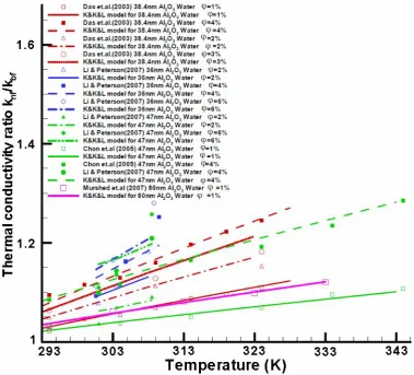
Of all the physical properties of nanofluids, the thermal conductivity is the most important one. For pure fluids, inherently low thermal conductivity is a primary limitation in high performance cooling which is the essential need of many industries. With the development of nanotechnologies, nanoparticles (i.e., particles of nanometer dimensions) can be produced. Nanofluids especially dilute suspensions of nanoparticles in liquids, exhibit ultrahigh heat transfer performance than the pure base fluids. Numerous experiments with nanofluids have shown the thermal conductivity enhancement of nanofluids (see Fig. 1.4 and Fig. 1.4), hence indicating promising applications to micro-scale cooling, e.g., impinging-jets cooling systems.

However, experimental findings have been controversial and theories did not fully explain the phenomenon of elevated thermal conductivity (see Koo and Kleinstreuer, 2004). Therefore, new thermal conductivity theory for nanofluids needs to be developed for better generalized agreement with experimental data of different types of nanofluids (i.e., metal-oxide nanofluids, metal nanofluids, etc).

Cooling is one of the top technical challenges being faced by high-tech industries, such as microelectronics, transportation, manufacturing and etc. Convective heat transfer to impinging-jets is well-known to yield high local and area averaged heat transfer coefficients. Impinging-jets are of particular interest in the cooling of electronic components furthermore in MEMS cooling.

3

observed enhancement of the thermal conductivity, knf, of nanofluids (Chapter 2), and

discusses simulation results of nanofluid flow in a radial microchannel using different knf

-models (Chapter 3). Specifically, Chapter 2 provides the derivation of the new Feng-Kleinstreuer (F-K) model as well as comparisons with benchmark experimental data sets and other theories focusing mainly on aluminum and copper oxide nanoparticles in water. The new thermal conductivity expression consists of a base-fluid static part, kbf, and a new

“micro-mixing” part, kmm, i.e., knf = kbf + kmm. While kbf relies on Maxwell’s theory, kmm

4

1.2

Motivations

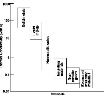
Instead of air-cooling systems, recently, liquid cooling technologies, e.g., immersion cooling, spray cooling for micro-scale devices such as chips have emerged. For better cooling effects, many ways to enhance heat transfer effects in cooling devices are investigated including changing flow geometry, boundary conditions, or by enhancing thermal conductivity of the fluid. The conventional way to enhance heat transfer properties of the fluid is to use conventional solid-liquid suspensions with millimeter- or micrometer-sized particles to replace pure fluids. Thermal conductivities of different materials are shown in Fig.1.1 (Das et al., 2008) and Table 1.1. However, millimeter- or micrometer-sized particle suspensions cannot be used in micro-scale devices cooling use because of the severe shortcomings, i.e., clogging effects and settling out of the suspensions. With the development of nanotechnologies, nanofluids are considered as the promising coolant cooling systems for micro-scale devices. Many experiments have reported the thermal conductivity enhancement of nanofluids than pure fluids. However, the controversies still exists for the mechanisms of such an enhancement effect and the relationships between thermal conductivity and parameters of nanofluids (i.e. temperature, volume fraction, and particle diameter, etc.). To find answers to the controversies, it is necessary to derive the expression of thermal conductivity for nanofluids from basic physical and fluid dynamics views.

5

6

1.3

Research Objectives

The objectives of this study are:

 To identify important mechanisms for nanofluid heat transfer properties enhancement;  To derive a new thermal conductivity model for nanofluids based on Brownian motion

micro-mixing mechanisms;

 To find a proper computational process to simulate nanofluid flow in closed impinging-jet cooling systems;

 To study thermal enhancement of nanofluid flow as applied to micro-scale impinging-jet cooling system;

7

1.4

Nanofluid Conduction Heat Transfer Properties

1.4.1 Experimental Methods and Observations

Nanofluids are a new class of heat transfer fluids by dispersing nanometer-sized particles with typical length scales on the order of 1 to 100 nm in traditional heat transfer fluids. The promising application of nanofluids as efficient coolants used in MEMS and other small scale apparatus is based on the anomalous thermal conductivity enhancement compared to the base fluids (i.e. water, ethylene glycol, et al.) which was discovered in experiments. Although Masuda et al. (1993) has shown different nanofluids (i.e., Al2O3-water, SiO2-water

and TiO2-wate nanofluids) have the increased thermal conductivity up to 30% in low volume

fraction (less than 4.3%), such a tremendous enhancement phenomenon was widely recognized firstly by Eastman and Choi (1997) for CuO-water, Al2O3-water and Cu-Oil

nanofluids using Transient Hot Wire method (THW). Also, after several years researches, the effective thermal conductivity (keff) was found has a relationship with several parameters (Yu

et al., 2008), i.e., nanoparticle material, particle volume fraction, particle size, particle shape, basic fluid material, temperature and pH value.

1.4.1.1 Experimental Methods

8

investigated as well as other static measuring methods. Additionally, according to many recent published papers, optical experimental methods are discussed either. Such a discussion is necessary since the enhancement trends of thermal conductivity of nanofluids due to different experimental methods differ from each other significantly.

1.4.1.1.1 Transient Hotwire Method (THW)

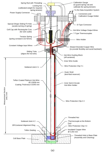
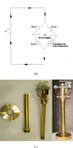
Transient hotwire method (THW) is the most widely used static, non-steady state, linear source experimental method for measuring the thermal conductivity of fluids. For this method, a hot wire is planted in the middle of the fluid (see Fig. 1.2 (a) and (c)). Such a hot wire is used both as a heat source and a temperature sensor. To the common sense based on Fourier’s law, when heating the hot wire, the higher the thermal conductivity of the fluid, the lower the temperature rise will be detected. Das et al. (2008) announced that since the experiment lasts for a maximum of 2 to 8 seconds which is a very short time interval, the natural convection cannot influence the accuracy of the result. The theoretical derivation of the relationship between the thermal conductivity knf and measured data T by THW are

presented as follows.

Assuming an infinitely long and thin, ideal continuous line source dissipating heat into an infinite medium, with constant heat generation (see Fig. 1.2 (a)). The energy equation in cylindrical coordinates thus can be written as:

1 1

nf

T T

r

t r r r



 _    

 

  _  _ (1.1)

9

T t( 0)T₀ (1.2 a)

0 lim 2 r nf T q r

r k



  _{ }  _ 

  and r 0

T

r _

 _

 (1.2 b and c)

Therefore, T can be solved and expressed as:

2

2 2

0 2

4 4

4

( , ) ln .. ...

4 1 1! 2 2!

nf nf nf nf r r t t t q

T r t T

k r       _{   }   _{   }                   _  _{ }_     _                 (1.3)

where  0.5772 which is the Euler’s constant. Hence, if the temperature of the hot wire at time t1 and t2 are T1 and T2,then by neglecting the high order terms, we can obtain the

thermal conductivity from Eq. (1.3):

1 2

1 2

ln( / ) 4 nf t t q k T T  

 (1.4)

For experimental measurements, the wire is heated with electrical constant power supply at step time. The temperature increase of the wire is determined from its change in resistance which can be measured in time using a Wheatstone bridge circuit (see Fig. 1.2 (b)). Thermal conductivity is determined from the heating power (or heat flux q) and the slope of curve ln(t) versus T.

10

device and procedure design may cause errors of the result either (e.g., tension on hot wire, suspend device for hot wire, etc). Accordingly, many revised hot wire methods and experimental designs are proposed. For example, Zhang et al. (2006) used short-hot-wire method (Woodfield et al., 2006) which can take into account of the boundary effects, Mintsa et al. (2009) add mixer into THW experimental devices thereby avoid the deposition of nanoparticles in the suspensions, and et al. Transient hot wire method is still the most popular measurement procedure because it is low cost, simple to operate, and easy to construct. Alternative static experimental methods are: temperature oscillation method (Das et al., 2003; Czarnetzki et al., 1995), micro-hot-strip method (Ju et al., 2008), steady-state cut-bar method (Li and Williams, 2008), 3-ω method (Choi et al., 2009), and radial heat flow method (Iyengar et al., 2009).

1.4.1.1.2 Optical methods

The latest experimental data for thermal conductivity of nanofluid is confusing, and contradictorily reported no anomalous enhancement. It leads to discussion that traditional methods such as the transient hot wire methods may suffer from practical drawbacks due to convective effects which may produce experimental data with large errors. To overcome such limits, alternative methods, i.e. optical methods were introduced.

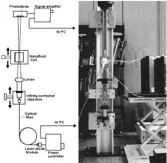
post-11

processing generate the thermal conductivity data. Compared to THW, this method separates the heating source and signal sensor, which avoid the interference. Rusconi (2006) reported no anomalous enhancement of thermal conductivity for nanofluids.

Similar to thermal-lensing (TL) method, optical technique of forced Rayleigh scattering (FRS) is demonstrated available to investigate thermal conductivity of well-dispersed nanofluids (Venerus et al., 1999 & 2006). Their results show no anomalous enhancement either for Au and Al2O3 nanofluids.

Furthermore, optical beam deflection technique is used to measure thermal conductivity of nanofluids (Putnam et al., 2004 & 2006). The nanofluid is heated by two parallel lines by square current. The schematic of optical beam deflection technique is provided by Putnam et al. (2004). The temperature change of nanofluids can be transformed to light signals captured by dual photodiode. Putnam et al. (2006) also reported no anomalous enhancement of thermal conductivity of nanofluids.

Besides the methods which are discussed above, there are many other thermal conductivity measurement methods, such as horizontal flat plate method, cylindrical source method, spherical source method, and plane source method, etc. Further experimental methods discussions are clearly needed to resolve the controversy over anomalous enhancements of thermal conductivity for nanofluids.

1.4.1.2 Experimental Observations

1.4.1.2.1knfvs. temperature (T)

12

temperature which showed nanofluids thermal conductivity will significantly increase with the increase of temperature. Patel et al. (2003) reconfirmed the findings of Lee et al. (1999) and Chon et al. (2005) and confirmed the temperature effect obtained by Das et al. (2003). They also showed the inverse dependence of particle size on the thermal conductivity enhancement with three sizes of alumina nanoparticles suspended in water.

However, there are many controversies on the temperature relationship. Since as usual, the thermal conductivity of base fluids will increase when the temperature increase, some experimentalists conclude that the effective thermal conductivity enhancement according to the temperature increase is only the effect of base fluid (Timofeeva et al., 2007). Furthermore, many scientists used optical measurement methods (Rusconi et al., 2006; Putnam et al., 2006; Venerus et al., 2006; Williams et al., 2008; Kolade et al., 2009) obtaining the effective thermal conductivities of nanofluids and found no anomalous effective thermal conductivity enhancement which leads to a doubt that if the anomalous enhancement is due to THW method. Meanwhile, Ju et al. (2008) systematically analyzed and commented on the error possibilities of THW method and investigated 20nm, 30nm and 45nm Al2O3 nanoparticle

water suspensions up to volume fraction 10% by micro hot strip method. Ju et al. (2008) did not discover strong relationship between effective thermal conductivity enhancement and temperature increase. The experimental data from classic and newly published papers (2008 & 2009) are compared in Fig. 1.5.

1.4.1.2.2 knfvs. volume fraction ()

13

comparing to the base fluid with very small nanoparticle volume fraction. Lee et al. (1999) investigated CuO-water/ethylene glycol nanofluids with particle diameter 18.6 nm and 23.6 nm as well as Al2O3-water/ethylene glycol nanofluids with particle diameter 24.4 nm and

38.4 nm and discovered a 20% thermal conductivity increase with volume fraction 4%. Wang et al. (1999) discovered 12% increase in keff by doing experiment on 28 nm-diameter Al2O3

-water and 23 nm-diameter CuO--water nanofluids with 3% volume fraction. Easterman et al. (2001) reported a tremendous 40% thermal conductivity increase for 10 nm-diameter Cu-water nanofluids with volume fraction only 0.3%. Li and Peterson et al. (2006) provided the thermal conductivity expression in terms of temperature (T) and volume fraction () by using curve fitting for CuO-water and Al2O3-water nanofluids. For other nanofluids, Xie et al.

(2002) investigated SiC-water nanofluids and Hong and Yang (2005) focused on Fe-water nanofluids. Recently, Chopkar et al. (2008) investigated Ag2Al-water nanofluids and Al2

Cu-water nanofluids and reported a 130% increase in thermal conductivity with only less than 1% particle volume fraction. Mintsa et al. (2009) provided new thermal conductivity expressions for Al2O3-water with particle diameters 47 nm and 36 nm individually and

measured thermal conductivity of CuO-water nanofluids either. Murshed et al. (2009) reported a 27% increase in 4% TiO2-water nanofluids with particle diameter 15 nm and 20%

increase for Al2O3-water nanofluids. However, Duangthongsuk et al. (2009 a) provided more

moderate increase for TiO2-water nanofluids. For these new experimental data around 2009,

14 1.4.1.2.3 knf vs. other parameters

There are other parameters which can influence knf either, e.g., pH value, different base

fluid materials and additives. Zhu et al. (2009) showed that the pH of the nanofluid strongly affects the thermal conductivity of the suspensions. For different based fluid materials, Water based nanofluids own higher thermal conductivities compared to ethylene glycol based nanofluids with the same nanoparticle volume fraction (Wang et al., 1999; Jang and Choi, 2004;Li and Peterson, 2006; Timofeeva et al., 2007), however, the thermal conductivity of ethylene glycol based nanofluids enhance faster than water based nanofluids (Lee et al.,1999;Wang et al., 1999). According to our knowledge, no big controversy exists in those experimental data. The pH influence should be validated by more papers in future. Additionally，different particle shapes can also influence the thermal conductivity of nanofluids. Nanoparticles with high aspect ratio seem to be helpful to enhance the thermal conductivity. For example, spherical particles shows slightly less enhancement than those containing nanorods (Murshed et al., 2005) and Thermal conductivity of CuO-water based nanofluids containing shuttle-like shaped CuO nanoparticles is larger than those for CuO nanofluids containing nearly spherical CuO nanoparticles (Zhu et al., 2007).

1.4.1.2.4 knf of other nanofluids

15

16

used, i.e., Convective heat transfer devices (Ding et al., 2006) and 3-method (Choi et al., 2009). No big difference on the enhancement of thermal conductivity is reported by using different experimental methods.

1.4.2 Numerical Methods and Observations

1.4.2.1 Direct Numerical Simulation

Direct numerical simulation is a way of solving solid-liquid flow interactions exactly, without approximations. The particles are controlled by Newton’s 2nd law submerged in the base fluids. One must simultaneously integrate the Navier-Stokes equations and the equations fo rigid-body motion (Koo, 2005). Direct numerical simulation (DNS) is recently used by Li and Peterson (2007) to evaluate the dominate mechanisms of the enhancement for nanofluid thermal conductivity. The mesh of the particle and the surrounding fluid are shown in Fig. 1.6 (Li and Peterson, 2007). By investigating one particle, three particles, and multi-particle cases in ANSYS-CFX 5.5.1, Li and Peterson presented the velocity field and temperature field, and visualized the superimposition of multi-particle effects. It needs to mention that Li and Peterson did not use Langevin equation as the supplementary equation which describes the Brownian motion of nanoparticles. Instead, they use general form of the wave equation with no damping. The governing equations are given as follows (Li and Peterson, 2007):

Continuity equation

0

y

x v z

v v

t x y z

   

 _{   }

17 Momentum Equations

2 2 2

2 2 2

x x x x x x x

x bf

v v v v p v v v

F

t x y z x x y z

_    _   _   _

       

    (1.6 a)

2 2 2

2 2 2

y y y y y y y

y bf

v v v v p v v v

F

t x y z x x y z

_ _ _ _  _  __ _ _ _

    (1.6 b)

2 2 2

2 2 2

z z z z z z z

z bf

v v v v p v v v

F

t x y z x x y z

_    _   _   _

       

    (1.6 c)

Energy Equation

 

p _bf bf bf bf bf

dT T T T

c k k k

dt x x y y z z

   _  _  _  _  _  _ 

            (1.7)

Particle motion equation

2

2 0

p

d x

m bx

dt   (1.8)

where b is a constant (or effective stiffness), and  is the diffusion matrix. Based on their numerical simulation results, a small temperature gradient can be observed compared to pure fluid situation, which indicates that the Brownian motion of nanoparticles could significantly affect the macro heat transfer properties of the nanofluids. However, the effect on the simulation results of using Eq. (1.8) instead of Langevin equation need to be further discussed.

1.4.2.2 Molecular Dynamics

18

heat transfer enhancement of nanofluids. For details, molecular dynamics (MD) is a form of computer simulation in which atoms and molecules are allowed to interact for a period of time by approximations of known physics, giving a view of the motion of the particles. It is promising to be used as technique as a microscope with high temporal and spatial resolution (Karniadakis, 2002). For nanofluid thermal conductivity numerical simulation, the algorithm of molecular dynamics (MD) can be briefly introduced as follows:

 Set up initial conditions and geometries of particles and surrounding fluid which are consist of atoms

 Give atoms initial positions, choose time step length

 Determine the interactions forces and external forces on each atoms

 Solve Newton’s 2nd

law for each atoms and update positions of atoms

 Solve energy equations and update temperatures

 Move to next time step and repeat iterations

In MD method, the interaction between particles or atoms is normally based on Lennard-Jones potential with various forms of expression. The original Lennard-Lennard-Jones potential is given by:

12 6

( ) 4

ij r

r r

 

    

  _{ } _{  }    

 

  (1.9)

19

cannot be captured by experiments, the accuracy of the results is strongly dependent on the parameters selections in the interaction potential.

1.4.2.3 Direct Simulation Monte Carlo (DSMC)

Direct simulation Monte Carlo (DSMC) is a direct particle simulation method based on kinetic theory and introduces random numbers. The method can be described as a method tracking a large number of statistically representative particles. The particles’ interactions are then used to modify their positions, velocities, temperatures or chemical reactions (Oran et al., 1998). DSMC is also able to take into account the particle interactions and particle-fluid interactions.

The essence of DSMC algorithm consists of four procedures:

 Move the particles

 Index and cross-reference the particles  Simulate collisions

 Statistically sample the variables in the field

Oran et al. (1998) presented detailed DSMC flowchart and applications in fluid flows. For nanofluid thermal conductivity numerical simulation, Feng et al. (2008) utilized DSMC method and investigated different types of nanofluids (e.g. CuO-water, Al2O3-water, and etc.)

20

1.4.3 Theoretical Models

The thermal conductivity of multiphase fluids started from the static model of Maxwell (1891) whose model is developed to determine the effective electrical or thermal conductivity of liquid-solid suspensions for low volume fraction mixtures with uniform particle spherical size. Hamilton and Crosser (1962) developed Maxwell’s result to non-spherical particles. For other classical models please refer to Jeffery (1973), Davis (1986) and Bruggeman (1935). Other classical models are presented in Table 1. The classical models originate from continuum formulations which typically involve only the particle size/shape and volume fraction and assume diffusive heat transfer in both fluid and solid phases (Wang, 2008). Although they can give good predictions for micrometer or larger-size multiphase systems, the classical models usually underestimate the enhancement of nanofluids thermal conductivity increase with volume fraction.

Differing from the classical models mentioned above which treat particles stationary to the base fluids, dynamical models are trying to take the effect of nanoparticles’ random motion into account. Since, nanoparticles are moving randomly, the dynamical models should be more realistic. The dynamical mechanisms of the anomalous thermal conductivity enhancement of nanofluids can be explained from four possible aspects (Keblinski et al., 2002):

(a) Brownian motion of nanoparticles

21

(d) The effect of nanoparticle clustering

New mechanisms can also be categorized into conduction, nano-scale convection, near-field radiation (Das et al., 2008), and thermal waves propagation (Wang et al., 2008). Since we will establish the new theoretical model based on the micro-mixing and micro-dissipation effect of nanoparticle Brownian motion, we narrowed our literature review to the theoretical model papers based on Brownian motion effects. Gupte et al. (1995) proposed a numerical approach (unit cell approach) to calculate uniform distributed micro particles’ falling velocity induced heat transfer effects. He gave the velocity function by using stream potential, and using finite difference method to solve the energy equation. The model of calculating velocity field is helpful for our new Feng-Kleinstreuer (F-K) model establishment. For other papers concerning about micro-particle motion (including rotation) induced heat transfer effects, see Leal et al. (1973) and Gupte et al. (1993).

After Masuda et al. (1993) and Eastman and Choi (1997) reported the anomalous increase of the effective thermal conductivity for dilute nanoparticle suspensions, many scientists started focusing on the contribution given by the Brownian motion of nanoparticles to such a phenomenon.

22

However, Wang et al. (1999) and Keblinski et al. (2002) failed to consider the surrounding fluid motion induced by the Brownian particles. Therefore, though they concluded Brownian motion effect is not the essential mechanisms many scientists are still working on the theoretical model establishment based on Brownian motion effects.

Jang and Choi (2004) focused on the heat transfer between nanoparticles and carrier fluid, proposed four modes of energy transport and introduced the idea that a Brownian nanoparticle produces a convection-like effect at the nano-scale. The effective thermal conductivity is written as

(1 ) 3 ₁ Re Pr

p

bf

nf bf p bf d

p

d

k k k C k

d

  

    (1.10)

where C1 is an empirical constant and dbf is the base fluid molecule diameter. Red_p is the

Reynolds number, defined by

Re p p p d bf v d   

 (1.11 a)

3

Boltzmann p

bf bf p

T D v d   

   (1.11 b)

where D is the nanoparticle diffusion coefficient, Boltzmann 1.3807e23J / Kis the Boltzmann

constant, vp is the root mean square velocity of particles and bfis the base fluid molecule

mean free path. However, Jang and Choi (2004) neglected the micro-mixing due to the random particle motion.

23

model. The former one separated the heat flow carried by base fluid and nanoparticle and the thermal conductivity is not a function of temperature. Hence, based on the experimental data which showed the relationship between knf and T , the latter moving particle model was

developed briefly and build a relationship between the effective thermal conductivity and the average particle velocity which is determined by the temperature T. However, Kumar et al. (2004) didn’t take the solid-fluid interaction effects into account.

Prasher et al. (2006) claimed the importance of Brownian motion on the enhancement of nanofluids thermal conductivity and suggested any models which are accurate in describing the multiphase fluid with larger particle sizes should revise when the particle sizes decreases to nanoscale. Based on Maxwell-Garmett thermal conductivity model and introducing correlations, The Multi-Sphere Brownian (MSB) model can be read as



1 Re Pr0.333



(1 2 ) 2 2 (1 2 )

(1 2 ) 2 (1 2 )

p m p m

nf m

bf p m p m

k k k k

k

A

k k k k k

  



  

_   _ _   _

 

  

 _   _ _   _ 

 

(1.12)

where Re is defined by Eq. (1.11a), 2R k_{b m}/d_p is the nanoparticle Biot number, and _{0.77 10}8 2_/

b

R    Km W for water-based nanofluids which is so called thermal interface resistance. A and m are empirical constants. As mentioned by Li (2008) and Kleinstreuer and Li (2008), MSBM model failed to predict the thermal conductivity enhancement trend when the particle was too small or too large. Also, because of the curve-fitting parameters A and m, Prasher’s model is lack of generality.

24

by two parts

k_nf k_statick_Brownian (1.13) where kstatic is static thermal conductivity due to the higher thermal conductivity nanoparticles

mixed into the based fluid which can be expressed as (Maxwell, 1904)

3 1 1 2 1 p bf static

bf _{d d}

bf bf

k

k k

k _{k k}

k k                                  (1.14) Brownian

k is the enhancement thermal conductivity part generated by the additionally convective heat transfer of particle’s Brownian motion and ambient fluid induced motion. Referring to the Stokes flow around a sphere, Koo (2005) determined the affected fluid volume. By introducing β and f(T,υ) two empirical functions, Koo (2005) combined the interaction between nanoparticles and temperature effect into the model and produced:

5 104 ( ) B ( , )

Brownian p bf

p p

T

k c f T

d



  



   (1.15)

Li (2008) revisited the model of Koo and Kleinstreuer (2004 and 2005), based on Brownian motion induced micro-mixing combined the functions  and f (T, ) into a new

g-function which considered the influence of particle diameter, temperature and volume fraction. The g-function is an empirical function changes with different types of nanofluids (Li, 2008). Also, by introducing a thermal interfacial resistance 8

f

R  4 10 km2/W the

25

,

p p

f

p p eff

d d

R

k k

  (1.16)

Therefore, the expression of KKL (Koo-Kleinstreuer-Li) model is

5 104 ( ) B ( , , )

Brownian p bf p

p p

T

k c g T d

d



  



   (1.17)

where g(T, ,d ) _p is written as









2

2

( , , ) ln( ) ln( ) ln( ) ln( ) ln( ) ln( )

ln( ) ln( ) ln( ) ln( ) ln( )

p p p p

p p p

g T d a b d c d d e d T

g h d i j d k d

  

 

     

    (1.18)

where a-k here are the empirical coefficients based on the type of particle-liquid pairing (Li, 2008). The KKL model determined the effective thermal conductivity as a function of temperature, volume fraction, particle size and etc. The base fluid properties substituted into Eq. (1.18) are also treated as a function of temperature T.

For newly published papers concerning about Brownian motion effect, Bao (2009) also considered the effective thermal conductivity consists of static part and Brownian motion part. Different from KKL model, he only focused on one time interval of Brownian motion which means the velocity of the particle is constant and treated the ambient fluid around nanoparticle steady flow. Considering convective heat transfer through the boundary of the ambient fluid which has the same definition as KKL model did, Bao (2009) provided an expression for Brownian motion thermal conductivity as a function of volume fraction, particle Brownian motion velocity vp and Brownian motion time interval  where vp can be

26

from the stochastic process description of Brownian motion. However, he didn’t consider the collision between nanoparticles which may influence the effective thermal conductivity either (see Chap. 2 for details).

In later chapters, we compared different effective thermal conductivity models with our new theory and substituted them into the calculation of nanofluids convective heat transfer in the cooling systems to see the accuracy of the model predictions.

1.5

Nanofluids Convective Heat Transfer Properties

Based on the tremendous enhancement in thermal conductivity, nanofluids are expected to be suitable for practical applications with little or no penalty in pressure drop. Also, the conventional convective heat transfer correlation of the pure fluid is not suitable for the nanofluids. Hence, the research on the convective heat transfer properties of nanofluids is necessary which should not only focus on the Nusselt number (Nu) and heat transfer coefficient (hnf), but also on friction factor, pressure drop, and effective viscosity of

27

Tw is supplied at the wall of the test section.

1.5.1 Heat transfer coefficient (h

nf

) and Nusselt number (Nu)

The heat transfer coefficient hnf comes from the Newton’s law of cooling, and is defined

for nanofluids as:

w nf

w b

q h

T T



 (1.19)

where qw is the wall heat flux, Tw is wall temperature, and Tb is the bulk temperature of fluid.

Based on hnf, Nusselt number of nanofluid is defined as: nf nf

nf

h D Nu

k

 (1.20)

which is the ratio of convective heat transfer to conductive heat transfer. Hence, the larger the Nusselt number is, the better convective heat transfer performance of the flow is. D is the characteristic length of flow (e.g., D is the pipe diameter for Hagen-Poiseuille flow). In Eq. (1.20), knf is usually given by in-house experimental data or by theoretical predictions.

1.5.1.1 Nusselt Number (Nu) for Pipe Flow of Conventional Fluid

For fully developed laminar pipe flow, Nusselt number Nu is given as (Kreith et al., 1993):

4.364 constant wall heat flux

Nu

3.66 constant wall temperature

  

 (1.21 a)

28

3.608 constant wall heat flux

Nu

2.976 constant wall temperature

  

 (1.21 b)

For turbulent flow, Dittus-Boelter equation can be used as correlation expression for Nu:

0.8

0.023Re Prn

Nu (1.21 c) where Re is the Reynolds number and Pr is Prandtl number. Especially, n=0.3 for cooling of the fluid and 0.4 for heating of the fluid. Dittus-Boelter equation is only valid for 0.7<Pr<160, Re>10000, and L/D>10 in which L is the pipe test section length and D is the pipe test section diameter. Other correlations for turbulent pipe flow are presented by Turns et al. (2006).

1.5.1.2 Experimental Data and Correlations for Nanofluid Pipe Flows

For nanofluids, Li et al. (2002) announced that Nusselt number Nunf can be expressed as

follows:

 

 

Re , Pr , p , p p , , , .

nf nf nf

bf p _nf

c k

Nu f Pe etc

k c             (1.22)

where Renf  

 

v D /nf is the Reynolds number of nanofluid , Prnf nf /nf is the Prandtl

number of nanofluid , Pe 



v d_p



/_nf is Peclet number, and _{nf nf} /

 

_p

nf

k c

   .

Pak and Cho et al. (1998) reported heat transfer data for turbulent flow of alumina/water and titania/water in pipe. Nunf is shown 30% higher than predicted by pure fluid correlation

i.e., Dittus-Boelter equation, for Al2O3-water nanofluid with particle diameter 13nm.

29 0.8 0.5

0.021Re Pr

nf

Nu  (1.23)

Li and Xuan (2002) investigated Cu-water nanofluid pipe flow with constant wall heat flux. Cu particle diameter is lower than 100nm. Their results showed the suspension of Cu nanoparticle remarkably enhanced the heat transfer performance than the conventional base fluid. Additionally, Li and Xuan (2002) proposed correlations for prediction of Nusselt number for nanofluids both in laminar and turbulent regions as:



0.754 0.218



0.333 0.4

0.4328 1.0 11.285 Re Pr

nf nf nf

Nu    Pe (1.24 a)



0.6886 0.001



0.9238 0.4

0.0059 1.0 7.6286 Re Pr

nf nf nf

Nu    Pe (1.24 b)

from where it is apparent to identify the relationship between Nusselt number and particle volume fraction of nanofluids. Interestingly, the relationship between Nu and Re is contradictory from conventional fluid analysis.

However, recently, Williams et al. (2008) reported no anomalous enhancement in convective heat transfer performance for dp =46nm spherical Al2O3-water nanofluid and dp

=60nm spherical ZrO2-water nanofluid. It may because of the larger particle diameters

30

convective heat transfer experimental researches on nanofluids focused on tube flows of nanofluids. However, for micro-scale flows, it is more popular and promising to investigate the convective heat transfer properties of rectangular duct flow and flow between parallel disks for practical use (i.e., cooling system).

In summary, Nusselt number of nanofluid is not only determined by Reynolds number and Prandtl number, but also determined by nanofluids parameters, i.e., volume fraction, particle diameter, and etc. New Feng-Kleinstreuer (F-K) model or correlation is needed to accurately combine all the relevant parameters.

1.5.2Viscosity of Nanofluids

1.5.2.1 Experimental Observations

Recent investigations indicate that not only the heat transfer characteristics but also the transport properties (i.e. dynamic viscosity) of nanofluids remarkably change compared with pure base fluids. By experiments, Wang et al. (1999) reported the viscosity of nanofluids increases with increasing volume fraction of particles while Li et al. (2002) reported the viscosity of nanofluids increase with decreasing the temperature of fluids. Also, shear thinning behavior was reported in different nanofluids for the relationship between nanofluid viscosities and shear rate (Ding et al., 2006). The experimental discoveries reveal that the viscosity of nanofluid is as complicated as the thermal conductivity.

1.5.2.2 Theories for the viscosity of nanofluids

31

particle does not overlap with other particles disturbance. The expression is:





eff 1 2.5 bf

     (1.25)

Afterwards, many expressions of the effective viscosity has been developed and proposed by taking into account the particle-particle interactions, non-spherical geometries of particles, and etc. (Wang et al., 2008). For example, Brinkman et al. (1952) has extended Einstein’s formula by using moderate particle concentrations,





eff 2.5 bf

1

1

 





 (1.26)

Lundgren et al. (1972) proposed the following equation with higher order terms of volume fraction to take into account the particle-particle interactions:

2 3

25

1 2.5 ( )

4

eff O bf

  _     _

  (1.27)

Batchelor et al. (1977) considered the effect of Brownian motion of particles, and proposed the new expression for effective viscosity as:



2



eff 1 2.5 6.5 bf

      (1.28)

32

To develop suitable expressions of viscosity for nanofluids, Koo and Kleinstreuer (2005) proposed a formula with empirical parameters as:



 



4

5 10 B 134.63 1722.3 0.4705 6.04

eff bf p p T T d       

  _     _ (1.29)

where  is the empirical parameter related to particle motion which is given by:









0.8229

0.7272

0.0137 100 0.01

0.0011 100 0.01

        _    

 (1.30)

Kulkarni (2006) developed an expression for copper oxide nanoparticles suspensions:



2

 

2







2.8751 53.548 107.12 1078.3 15857 20587 1/

eff T

          (1.31)

From above theoretical derivations which are developed for nanofluids, the relationship between viscosity and temperatures are still in controversies (see Eqs. (1.29) and (1.31)).

Also, there are plenty of papers provided expressions for nanofluids based on the experimental data curve fitting techniques (Maiga et al., 2004 & 2005; Nguyen et al., 2007). For systematically research on Al2O3-water and CuO-water nanofluids, Nguyen et al. (2007)

obtained several expressions for different particle diameters and temperatures. For example, for Al2O3-water with particle diameters 47nm and 36nm, and CuO-water with particle

diameter 29nm at ambient temperature respectively, the viscosities can be given by:

eff

bf

0.904 exp(0.148 )

 _

  (1.32)

2 eff

bf

1 0.025 0.015

 _{ }

33

2 3

eff

bf

1.475 0.319 0.051 0.009

 _{  }

     (1.34)

For relationship with temperature in oC, Nguyen et al. (2007) obtained two expressions for 1% and 4% volume fraction nanofluids as follows:

1.1250 0.0007

eff bf

T



   (1.35)

2

2.1275 0.0215 0.0002

eff bf

T T



    (1.36) Moreover, for TiO2-water nanofluids, Duangthongsuk et al. (2009 a) reported quite

different viscosities compared to other existing papers, and proposed an equation for predicting the viscosity of TiO2-water nanofluids for different temperature and volume

fractions as follows:

eff 2

bf

a b c



 

    (1.37)

where a, b, and c are constants changes with temperatures, i.e., 15oC, 25oC, and 35oC (Duangthongsuk et al., 2009 a).

34

a side-effect.

1.5.3 Friction factor (f

nf

) and pressure drop

According to existed papers, most of the friction factor and pressure drop researches on nanofluid are focused on circular pipe flows either. The friction factor (f) can be derived from both differential approach and integral approach for Hagen-Poiseuille flow (Panton, 2005), and obtained by correlation from Moody chart (Turns et al., 2006). The Darcy-Moody friction factor fD can be defined as (Turns et al., 2006):

2

4 1 2

w D

f

v

 

 (1.38)

where _wis shear stress at the wall, is the fluid density, andvis the average velocity of the flow. An alternative friction factor is defined as Fanning friction factor (fF):

4

D F

f

f  (1.39)

1.5.3.1 Friction factor and pressure drop for pipe flow

Specifically, for laminar Hagen-Poisuille flow f_D can be calculated as:

64 Re

D

f  (1.40)

where Re

 

vD /is the Reynolds number of the fluid.

35 0.25

0.316 Re

D

f   (1.41) which is suitable for 4000<Re<105. Haaland correlated from Moody chart and provided an expression for f_D as:

1.11

1/ 2 6.9 /

1.8ln

Re 3.7

D

D

f    _ _ 

 

 

  (1.42)

where   _turb/ is the kinematic eddy viscosity of fluid and _turbis the apparent turbulent viscosity.

In pipe flow, the pressure drop can be expressed in terms of friction factorf_D:

2

2

D

L v

p f g

D



  (1.43)

where L is the length of the pressure drop test section, and g is the acceleration caused by gravity. For laminar pipe flow, by substituting Eq. (1.40) into Eq. (1.43), it produces:

2

32 Lv

p D



  (1.44)

1.5.3.2 Friction factor (fnf) and pressure drop (∆pnf) for nanofluids

36

Heris et al. (2007) investigated the convective heat transfer properties of Al2O3-water

nanofluid and shoed good agreement exists between pressure drop of the nanofluid and theoretical results (see Eq. (1.44)). Similar comparison results are obtained by Williams et al. (2008) for Al2O3-water and ZrO2-water nanofluids. For turbulent flow region,

Duangthongsuk et al. (2009) measured pressure drops of TiO2-water nanofluid in different

temperatures. The experimental results show the conventional single-phase pressure drop correlation is available for nanofluids. For rectangular microchannel flow, Jung et al. (2009) announced good agreement between friction factor fnf for Al2O3-water versus Reynolds

number and friction factor f for pure water versus Reynolds number. And the relationship between fnf and Re is closed to theoretical value from correlation (Jung et al., 2008):

56.9 Re

nf

f  (1.45)

More convective heat transfer researches need to be done for rectangular microchannel nanofluid flow and other types of flow which have promising applications in MEMS.

37

Kleinstreuer (2008) analyzed the thermal performance of nanofluid flow in a trapezoidal microchannel using pure water and CuO-water with volume fractions of 1% and 4%. The results show that nanofluids do measurably enhance the thermal performance of microchannel mixture flow with a small increase in pumping power. The thermal performance increases with volume fraction; but, the extra pressure drop, or pumping power, will somewhat decrease the beneficial effects. Microchannel heat sinks with nanofluids are expected to be good candidates for the next generation of cooling devices.

1.6

Impinging-jet cooling systems

1.6.1 Impinging-jets applications

38

1.6.2 Convective heat transfer properties of impinging-jets

1.6.2.1 Conventional fluid radial flows between parallel disks