Division V
“NORMAL” AND “ABNORMAL” DAMPING EFFECT ON THE
RESPONSE SPECTRA
Alexander Tyapin1
1
Chief Specialist, JSC ATOMENERGOPROJECT, Russia
ABSTRACT
Specialists working in earthquake engineering generally are sure that the increase in damping causes the decrease in response; e.g. response spectra for increasing damping decrease in the whole frequency range. Hence, the underestimation of damping in the analysis leads to the conservative results. The author shows that even the elementary SDOF oscillators sometimes in certain frequency ranges demonstrate “abnormal” effect of damping on the dynamic response (i.e. response increases along with the increase of damping). For the modes with frequencies in such frequency ranges, the underestimation of modal damping leads to the underestimation of response. This effect is more pronounced for the narrow-banded excitations. Broad-banded excitation mitigates this effect, shifting the frequency range of the abnormal damping effect to the low natural frequencies of oscillators. The abnormal damping effects may be of special importance in two special cases: for seismo-isolated structures with very low natural frequencies, and for high-frequency dynamic excitations (like aircraft impact).
INTRODUCTION
Specialists working in earthquake engineering are accustomed to the fact that the increase in damping causes the decrease in response; e.g. the response spectra for increasing damping in oscillators decrease in the whole frequency range. Let us call such a situation “normal”, and the opposite situation – “abnormal” damping effect.
One of the consequences of “normal” damping effect is that the response spectra for the same time-history, but for the different damping coefficients are enveloping each other (giving the same PGA for the zero natural period). Calculations of the response spectra usually support this thesis (but not always – see below).
Another consequence is that the artificial underestimation of damping in the analysis always leads to the conservative results. This thesis is often used to justify the Rayleigh damping model. With this model all natural modes with natural frequencies falling into the range between two “Rayleigh frequencies” get the underestimated modal damping coefficients; common view is that the corresponding modal response becomes conservative.
This view about the “normal” damping effect is so common that it is extended to the dynamic excitations of different nature and different frequency content (e.g., airplane impact or blast wave).
The author has shared this view himself for many years. However, some years ago the author found out that the underestimation of damping not always leads to the conservative results (see Tyapin (2013-1)). At that time the author explained this result by phase combination of different modal responses in the multi-degrees–of-freedom system. For a stand-alone modal response (e.g., in the spectral theory) the author was still sure in the “normal” damping effect.
RESPONSE OF SDOF OSCILLATOR
Let us start with the simplest platform model: SDOF oscillator with viscous damping resting on the platform excited by acceleration a(t). Equation of motion written in the relative displacements X(t) is well-known:
) (
2 0X 02X a t
X
(1)Here ω0 is a natural frequency of the undamped oscillator; λ is a dimensionless damping
coefficient (as related to critical damping). In the frequency domain the transfer function T(ω) from the platform to the mass is given by the Equation
0 2 2 0 2 2 1 ) (
i T (2)Here ω is a current frequency; i is an imaginary unit. From Equation 2 one can find the second degree of the absolute value of complex transfer function T(ω):
2 0 2 2 2 0 2 0 4 0 2 ) 2 ( ) ( ) 2 ( ) (
T (3)This absolute value is equal to the unit (i.e. numerator in Equation 3 is equal to denominator) for the two values of the current frequency ω: first, for zero; second, for ω1=ω0 х 2
1/2
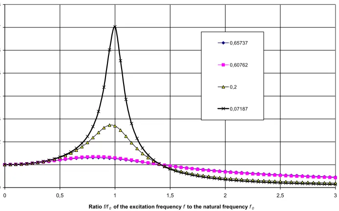
. Note that this second value (let us call it “the second natural frequency of oscillator”; the first one is a conventional natural frequency ω0) does not depend on damping. The curves for the absolute value of the transfer function for
different values of damping coefficient λ are shown on Figure 1.
Absolute Values of Transfer Functions
0 1 2 3 4 5 6 7 8
0 0,5 1 1,5 2 2,5 3
Ratio f/f0 of the excitation frequency f to the natural frequency f0
0,65737
0,60762
0,2
0,07187
These four values of damping coefficient λ correspond to the modal coefficients calculated in Tyapin (2012) for the sample soil-structure system considered further.
We see that the whole frequency range is divided not in two parts, but in three parts instead. Let us describe them from the left to the right:
1. Sub-critical range (excitation frequency ω is less than natural frequency ω0);
2. Near-critical range (excitation frequency ω is between the natural frequency ω0 and the
second natural frequency ω1, equal to the first natural frequency ω0 multiplied by the
square root of two);
3. Over-critical range (excitation frequency ω is greater than the second natural frequency ω1).
In the first two ranges the damping effect is “normal”; in the third range it is “abnormal”. This is a well-known result – one can find it for example on page 103 of Bolotin et al (1978). There is a special comment after the figure in this book stressing the increase of response with the increase of damping in the high frequency range of excitation (i.e. the “abnormal” damping effect).
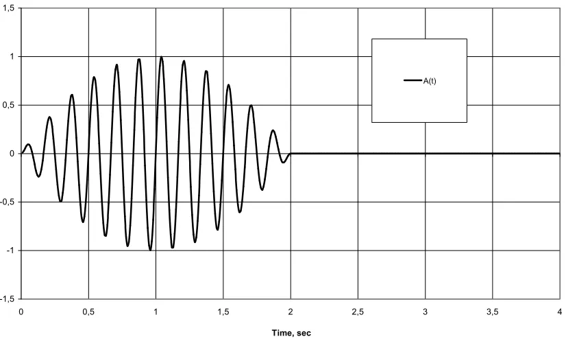
One can object that transfer functions describe the response to the harmonic excitation infinite in duration. However, the author has shown in Tyapin (2013-2) that harmonic excitation can be multiplied by a low-frequency “shape function” of finite duration leading to the excitation of finite duration. The example of such a narrow-banded (“almost harmonic”) excitation is shown in Figure 2.
Narrow-Banded Excitation
-1,5 -1 -0,5 0 0,5 1 1,5
0 0,5 1 1,5 2 2,5 3 3,5 4
Time, sec
A(t)
Figure 2. Example of narrow-banded excitation of the finite duration.
The same three frequency ranges may be described in other words, if we fix the excitation frequency and vary the natural frequency of oscillator. The same ranges will now go from the right to the left:
1. Sub-critical range (the natural frequency is greater that the excitation frequency);
3. Over-critical range (the natural frequency is less than the second excitation frequency).
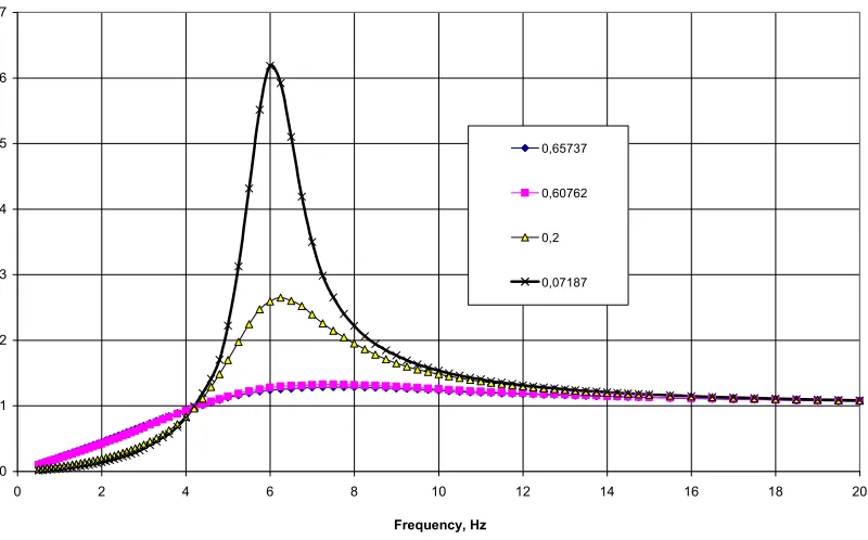
As above, in the two first listed frequency ranges we get “normal” damping effect; in the over-critical range we get the “abnormal” damping effect. This format enables the transfer to the response spectra. In Figure 3 one can see acceleration spectra for the excitation with dominant frequency 6 Hz shown in Figure 2. Damping values are the same as in Figure 1.
Spectra of the Narrow-Banded Excitation
0 1 2 3 4 5 6 7
0 2 4 6 8 10 12 14 16 18 20
Frequency, Hz
0,65737
0,60762
0,2
0,07187
Figure 3. Response spectra of the narrow-banded excitation with dominant frequency 6 Hz.
One can see in Figure 3 that the frequency range of the “abnormal damping” corresponds to the frequency range where spectral acceleration is less than peak ground acceleration (PGA). The same effect for transfer functions was in Figure 1.
The conclusion is that for narrow-banded excitations there exists a low-frequency spectral range (i.e. with low natural frequencies of oscillators) with “abnormal” damping effect. This conclusion may be valuable for the first modal responses to the high-frequency excitations like airplane crash. Another situation: seismo-isolated structures with very low first natural frequencies due to the special design of supports. In such situations the underestimation of modal damping leads to the non-conservative results in response calculated both by time-domain integration or spectral method.
BROAD-BANDED EXCITATION
Broad-Banded Excitation
-0,5 -0,4 -0,3 -0,2 -0,1 0,0 0,1 0,2 0,3 0,4 0,5
0,0 1,0 2,0 3,0 4,0 5,0 6,0
Time, sec
A(t)
Figure 4. Broad-banded seismic excitation.
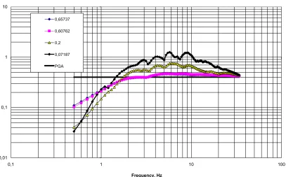
Spectra of the Broad-Banded Excitation
0,01 0,1 1 10
0,1 1 10 100
Frequency, Hz 0,65737
0,60762
0,2
0,07187
PGA
Comparing Figure 5 to the Figure 3 one can see a principal difference: spectral curves in Figure 5 do not have a single cross-section as in Figure 3. The range of the “abnormal” damping effect depends on the damping value. For high damping (two highest values about 0.6) this effect is seen up to 1.6 Hz – i.e. not far from the cross section point with horizontal straight line, corresponding to PGA. For the low damping values (0.2 and 0.0719) “abnormal” damping effect does not disappear, but the frequency range is shifted to the lower frequencies: at 0.5 Hz the damping effect is abnormal, but at 0.6 Hz it is normal.
Here one can find the explanation of the above mentioned common belief in the “normal” damping effect: for broad-banded excitations and the conventional low damping values the frequency range of the “abnormal” damping effect lies at the low frequencies where spectra are seldom calculated.
Why the difference between narrow-banded and broad-banded excitations is so great here? The author suggests the following explanation as a hypothesis. For given natural frequency of oscillator the response to a broad-banded excitation is a combination of responses to narrow-banded excitations with different dominant frequencies. Part of these narrow-banded components corresponds to the “normal” damping effect, another part – to the “abnormal” damping effect, depending of the ratio of dominant excitation frequencies to the second frequency of oscillator.
Let us compare the difference in spectra in Figure 3 for low damping (0.07 and 0.2) in “normal” frequency range (say, near 6 Hz) and in “abnormal” frequency range (say, near 4 Hz). In the first case the difference is higher. It means that even a small-magnitude component in “normal” range can compensate the effect of a component in “abnormal” range with higher magnitude. The less is damping the greater is a potential for such compensation. That is why the low-frequency components of broad-banded seismic excitation, though small in magnitude, for low damping cause the “normal” damping effect shifting the border of an “abnormal” range in Figure 5 to the left.
Thus the frequency content of excitation is of crucial importance for the damping effect. Probably there exists the frequency content, completely excluding “abnormal” damping effect for certain low damping values.
For a given excitation and given damping coefficients λ1 and λ2 one can calculate a frequency
fa(λ1,λ2), where spectrum for λ2 crosses spectrum for λ1. For the case shown in Figure 5 fa(0.07187;
0.2)=0.6 Hz, and fa(0.07187; 0.60762)=0.95 Hz. Limit of this frequency for value of λ2 approaching λ1
(let us call it Fa(λ1)) shows the lower boundary of the frequency range where damping effect keeps
“normal”.
One can note that the “abnormal” damping in the above mentioned cases is seen in the frequency range where spectral accelerations are comparatively small – they are less than PGA and far less than spectral peaks. In response the author would like to remind that in order to get nodal loads in the spectral method spectral accelerations are multiplied not only by masses, but also by coefficients depending on modes (e.g., see Russian civil codes SP-14.13330.2014). Limited number of modes usually controls the response due to these coefficients, sometimes in spite of comparatively small corresponding spectral accelerations. If corresponding natural frequencies for these modes fall into the “abnormal” range (for the given excitation time-history) the whole response may appear to be “abnormal”. Spectral approach is not impossible in such case, but some of the assumptions may become dangerous in terms of conservatism.
CONCLUSIONS
The results obtained in this paper demonstrate that the “abnormal” damping effect (i.e. the increase of the response with the increase of damping) is not an exception; it is a rule but acting in certain frequency range only. In terms of response spectra this is a range of small natural frequencies. This range depends on particular excitation time-history and particular damping. For the modes with natural frequencies falling into this range the underestimation of modal damping leads to the underestimation of the response – i.e. to the non-conservatism.
be special situations (e.g., seismo-isolated structures with very low natural frequencies; or the impact of light airplane where dominant frequencies of excitations are far greater than main natural frequencies) when the “abnormal” damping effect may be important.
The main conclusion is as follows. When one is going to underestimate modal damping (in Rayleigh model or somehow else) he must prove that such underestimate is not leading to the non-conservatism due to the “abnormal” damping effect. To show this one should calculate (at least in doubtful situations) not a single spectrum of excitation but several spectra for different damping values. The author recommends to calculate Fa
(λ
1) for given excitation history.
REFERENCES
Tyapin A.G. (2013). “Damping in Modal Approach. Part III: Paradox with Cut-off in Modal Damping,”
Earthquake Engineering. Structural Safety, Russia, 2, 36-40 (in Russian).
Tyapin A.G. (2012). “Damping in Direct and Modal Methods: Effect of the Artificial cut-off of the Damping Coefficients,” Earthquake Engineering. Structural Safety, Russia, 4, 29-35 (in Russian). Bolotin V.V. et al. (1978). Vibration in Technique: Handbook. Volume 1. Vibrations in Linear Systems.
Mashinostroyeniye, Russia (in Russian).
Tyapin A.G. (2013). “Damping in Direct and Modal Methods. Part II: Changing of Material Structural Damping for Rayleigh Damping,” Earthquake Engineering. Structural Safety, Russia, 1, 21-28 (in Russian).