©
DOI: 10.1534/genetics.104.034199
Bayesian Estimation of Recent Migration Rates After a Spatial Expansion
Grant Hamilton,* Mathias Currat,*
,†Nicolas Ray,*
,†Gerald Heckel,*
Mark Beaumont
‡and Laurent Excoffier*
,1*Computational and Molecular Population Genetics Lab, Zoological Institute, University of Bern, 3012 Bern, Switzerland, †Genetics and Biometry Laboratory, Department of Anthropology and Ecology, University of Geneva,
1211 Geneva 24, Switzerland and‡School of Animal and Microbial Sciences, University of Reading, Reading RG6 6AJ, United Kingdom
Manuscript received August 1, 2004 Accepted for publication January 21, 2005
ABSTRACT
Approximate Bayesian computation (ABC) is a highly flexible technique that allows the estimation of parameters under demographic models that are too complex to be handled by full-likelihood methods. We assess the utility of this method to estimate the parameters of range expansion in a two-dimensional stepping-stone model, using samples from either a single deme or multiple demes. A minor modification to the ABC procedure is introduced, which leads to an improvement in the accuracy of estimation. The method is then used to estimate the expansion time and migration rates for five natural common vole populations in Switzerland typed for a sex-linked marker and a nuclear marker. Estimates based on both markers suggest that expansion occurred⬍10,000 years ago, after the most recent glaciation, and that migration rates are strongly male biased.
M
AKING quantitative inferences on molecular data of models that more closely reflect the complexity of real processes, potentially allowing the estimation of more in complex demographic settings remains anon-going challenge. Traditionally, inferences have been meaningful biological parameters.
Many species have had a complex history that has made using summary statistics under simplified models
(e.g.,FuandChakraborty1998). While sometimes use- included a spatial expansion from a restricted range (e.g., an expansionary period following an ice age), with ful for qualitative comparisons, these simple models do
not adequately reflect the complexity of processes that the establishment of new demes and the exchange of genes among those demes (Hewitt 2000; Ray et al. might affect molecular genetic diversity. Recent advances
2003;Excoffier2004). Although these expansion pro-in maximum-likelihood and Bayesian approaches have
cesses affect various aspects of molecular diversity differ-shown that it is possible to make full use of the data
ently and can thus be described using a combination of gathered from population samples (e.g.,Beaumont1999;
summary statistics, making joint estimates of expansion
Beerli and Felsenstein 2001; Nielsen and Wakely
parameters in an explicitly spatial setting would be
diffi-2001; Wang and Whitlock 2003). Although these
cult using either full-likelihood or more conventional methods have the potential to be accurate, the
calcula-methods. However, it may be possible to use an ABC tion of likelihoods under complex models can be
prob-approach to simultaneously infer spatial expansion pa-lematic, necessitating the use of simplified demographic
rameters in the context of an appropriate spatial model. models. A promising alternative approach is to compare
Additionally, data from differently inherited molecular summary statistics that are calculated from observed
markers can be used to investigate interesting biological data and related to the parameter(s) of interest, with
phenomena such as differences in dispersal rates be-summary statistics simulated under a model for which
tween the sexes after a range expansion. the parameters are known (e.g.,FuandLi1997;Tavare´
The purpose of this study is to show that an
approxi-et al. 1997; Pritchard et al. 1999; Estoupet al. 2001,
mate Bayesian approach can be used to accurately infer 2004;EstoupandClegg2003). An appealing feature
parameters of spatial expansion in a two-dimensional of these approximate Bayesian computational (ABC)
stepping-stone (2DSS) model, using both mtDNA se-methods is that models of any complexity can be used,
quences and short tandem repeats (STRs) as molecular provided only that data can be simulated under the
markers. We test the method using a range of parameter model (Beaumontet al. 2002). This allows for the use
combinations and also show that sampling from several demes rather than from a single deme improves estima-tion accuracy. Finally, we challenge the method with 1Corresponding author:Computational and Molecular Population
Ge-empirical data from natural populations of the common
netics Lab, Zoological Institute, University of Bern, Baltzerstrasse 6,
3012 Bern, Switzerland. E-mail: [email protected] vole (Microtus arvalis) to assess differences between male
tween the “observed” valuess1ands2and the simulated values
and female dispersal levels and to determine the time
of the same statisticss⬘1ands⬘2can then be found simply as
since the most recent range expansion.
␦i⫽√w*i1(s1⫺s⬘1)2⫹w*i2(s2⫺s⬘2)2, (2) MATERIALS AND METHODS where the index i emphasizes the fact that the Euclidean distances between simulated and observed statistics will differ
Estimation procedure and simulation model:We follow the
depending on the parameter to be estimated. Note that a ABC approach described formally byBeaumontet al. (2002)
weighting scheme using simplyR2was also investigated, but and briefly below. The method relies on the simulation of
did not lead to drastic differences to the present weighting large numbers of data sets using known parameters under a
scheme. Compared toR2, an advantage of the weighting in given model. Summary statistics are calculated for each data
Equation 1 is that it will enhance the difference in weight set. These simulated statistics are then compared with
sum-between parameter-statistic pairs with a strong relationship mary statistics calculated from the observed sample. Simulated
(R2⬎0.8) and those with a poor relationship, ensuring that summary statistics that are “close” enough (i.e., fall within a
most weight is placed on statistics with large determination predetermined distance,␦) to the observed summary statistics
coefficients. After the weighting step, each parameter is inde-are retained, with their associated parameters. All other data
pendently estimated in a way similar to that of the standard sets are rejected. After a smooth weighting and local regression
ABC multivariate local regression approach. Apart from the adjustment step, the accepted parameters form an
approxi-use of a WED, our estimation procedure differs from that of mate posterior distribution that can be used to estimate the
Beaumont et al. (2002) only in that we separate the time-parameter of interest.
consuming simulation stage from the estimation procedure.
Modification to conventional ABC :One aspect of
simultane-The modified algorithm is : (1) select prior distributions for ously estimating several parameters with the ABC method is
parameters⌽1and⌽2; (2) draw values⌽⬘1and⌽⬘2for⌽1and that while a statistic may estimate a given parameter well, it
⌽2from the appropriate priors ; (3) use⌽⬘1and⌽⬘2to simulate may be a poor estimator for other parameters. This problem
genetic diversity under the chosen model to produce a single has the potential to lead to a decrease in the accuracy of
data set, using the same genetic marker, number of samples, estimation. For instance, while variance in the size of STR
and number of loci as the observed data; (4) calculate the alleles evolving under a stepwise mutation model shows a
summary statistics valuess⬘1ands⬘2for the data set; (5) repeat strong relationship with the scaled expansion time ()
steps 2–4 until the desired number of simulations has been (Goldsteinet al. 1999), it carries little information on gene
completed; (6) compute summary statisticss1and s2on ob-flow. Conversely, it would be expected that the scaled
migra-served data; (7) choose a tolerance levelP␦to determine the tion rateM⫽2Nm(whereNis the number of genes present
number of data points retained for posterior density estima-in a local deme and mis the immigration rate from
neigh-tion; (8) forS1, retain a small proportion (e.g., 1%) of the boring demes) would show a stronger relationship with FST
s⬘1that are closest tos1together with their associated parame-than, for example, the mean number of pairwise differences
ters⌽⬘1; (9) regress the retaineds⬘1on⌽⬘1and obtain theR2 among mtDNA sequences (Excoffier2004). Thus while
sta-value; (10) repeat steps 8 and 9 forS2and calculate weights tistics are chosen because they describe well one aspect of a
w*⌽
1S1andw*⌽1S2using Equation 1 and scaling described above; range-expansion phenomenon, they will usually be less
infor-(11) calculate the WEDs between each simulated data set mative on other parameters. We address this issue by using a
usingw*⌽
1S1andw*⌽1S2and the observed data as in Equation weighting scheme such that statistics carrying more
informa-2, and retain a fractionP␦of the data sets (summary statistics tion on the parameter of interest are given a greater weight.
with associated parameters) that are closest to the observed
Beaumontet al.(2002) defined the distance␦using a
Euclid-data; (12) perform multiple regression of the retained statistics ean metric to give circular acceptance regions, accepting a
on the parameters and adjust posterior density as described proportionP␦of the simulation data (the tolerance). To aid
inBeaumontet al. (2002); and (13) repeat steps 8–12 for⌽2. estimation efficiency, we use a weighted Euclidean distance
The difference in analysis time between the simultaneous (WED). We assess the relationship between each
parameter-estimation of parameters under the standard ABC method statistic pair during a preliminary analysis step, in which a
and the extended method described above in which parame-local regression is run in the vicinity of each observed summary
ters are estimated in succession is small, being in the order statistic. The square of the correlation coefficient between a
of seconds to several minutes for a single set of observed data, parameter and a statistic (R2) from each local regression was
depending on the size of the simulation file. Also the time taken as a simple measure of the utility of the statistic to
necessary for computing the weights is negligible compared act as an estimator of the parameter in that region of the
distribution. to the time required for the simulations and the rest of the
For illustration, consider just two statistics,S1andS2, that estimation procedure. A comparison between the standard are believed to be informative for the parameter ⌽1, with ABC method and the extended method using a WED was valuess1ands2calculated for an observed data set (this proce- conducted using the demographic model, summary statistics, dure could of course be extended to more than two statistics). and priors that are described below.
To calculate the weight forS1for this observed data set, simu- Simulations:The simulation model is a modification of the lated statistics that are in the vicinity ofs1(for example, the model described byRayet al. (2003). A subdivided population 1% of the empirical distribution closest tos1) are collected, was simulated on a torus of 50-by-50 demes with an expansion together with their associated parameters. The retained statis- from an originating deme arbitrarily located at具25, 25典.Ray
tics are regressed on the retained parameters, allowing the et al. (2003) simulated a forward demographic expansion in
weight to be calculated as which colonization occurs as a wave from the originating
deme, with an ongoing exchange of migrants among demes wi j⫽ ⫺log(1⫺R2i j) , (1) that have been colonized [range expansion (RE) model]. Our
simulation model differs from the RE model, making the whereR2
i jis the determination coefficient of theith
param-common assumption of an instantaneous expansion, such that eter by thejth statistic. After the operation is repeated for S2,
each of the 2500 demes is filled instantly to a given size N the weights are scaled so as to sum to unity as w*i j ⫽wi j/
a deme) identical for all demes [instantaneous expansion (IE) model]. This slight modification allowed for much faster simulations. Under this model, neighboring demes exchange genes at a rate m during the T generations following the expansion and a standard backward coalescent process is im-plemented to simulate gene genealogies. During this back-ward process, gene lineages can either migrate between differ-ent demes or coalesce if they are in the same deme. Going backward in time, the instantaneous expansion corresponds to an instantaneous contraction, where all gene lineages are instantaneously brought back to the originating deme, where further coalescent events can occur until only one lineage remains. Genetic data are obtained by adding mutations at rateunder a strict stepwise mutation model for STRs and
a finite sites model without transition bias for sequences. Pa- Figure1.—A plot of RMSE for estimates of the migration rameters describing the scaled expansion time ⫽2T, the parameterM vs.tolerance (P␦). Tolerance represents here scaled population size ⫽ 2N, and the scaled migration the fraction of simulations retained for parameter estimation. rateM ⫽ 2Nm are thus known and are recorded for each Estimates using the standard ABC method are shown as open simulation. We note here the advantage of separating the squares, and those using the modified weighted Euclidean simulation model from the estimation procedure. Since the distance are shown as solid diamonds. One million simulations accuracy of estimation depends in part on the number of were used for each estimation. Bootstrapped standard errors simulations used (the simulation size), where possible it is were calculated on 10,000 replicates and are reported here desirable to use several hundreds of thousands to millions of around point estimates.
simulations. Depending on the complexity of the underlying demographic model, it therefore takes much longer to gener-ate the simulation file than to run the ABC estimation
proce-simulated parameters before the regression adjustment, and dure. During the exploration phase of research, the separation
parameter estimates were based on the back-transformed val-of these two steps saves considerable time by allowing multiple
ues. We also followBeaumontet al. (2002; Equation 7) in analyses to be run using a single simulation file.
using the fitted value of the regression line as a point estimate
Samples and summary statistics:Samples were drawn from
of the parameter. During exploratory analysis of a small subset three demes on the torus, which were located arbitrarily at
of results, means, medians, and modes of the posterior distri-具10, 40典,具30, 30典, and具40, 15典(identified hereafter as demes
bution were calculated as alternative estimators, and only mi-1, 2, and 3, respectively). There were at least 10 demes between
nor differences in the value of parameter estimates were each of the sampling demes. Fifty genes were drawn from
found. each sampled deme, consisting of either DNA sequences (300
bp) or nuclear STRs (10 independent loci), which were used to calculate summary statistics. For mtDNA, four within-deme
RESULTS summary statistics were calculated for each sampled deme:
number of haplotypes,k; homozygosity,Ho; number of segre- Simulation studies—modified vs. standard ABC:The gating sites,S; and the average number of pairwise differences,
accuracy of estimation under the ABC procedure de-. For STR data, three within-deme summary statistics were
tailed by Beaumont et al. (2002) depends on several
calculated for each sampled deme: mean number of alleles
per locus, a; homozygosity,Ho; and mean variance (across factors, including the simulation size, the number of
loci) in allele repeat number. The fixation index, FST, was parameters to estimate, and the tolerance. For a given calculated among demes for both markers whenever more simulation size, increasing the number of parameters than one deme was sampled. These statistics were chosen for
requires an increase in the tolerance. To determine if
their ability to estimate parameters on the basis of preliminary
using a WED increased estimation efficiency across a
investigations and their known dependency on the values of
range of tolerance values, compared with a standard
the parameters of a range expansion under the infinite island
model (Excoffier2004). ABC approach under the 2DSS model, the two methods
Parameter estimation:For mtDNA, simulations were sam- were assessed as follows. An observation set of sequences
pled from prior distributions ofas a uniform distribution
was generated under parameters ⫽ 10, ⫽ 5, and
between 0 and 50, as a log-uniform distribution between
M ⫽ 10. Here, and in subsequent evaluations, each
0.01 and 10, andMas a log-uniform distribution between 0.01
observation set consisted of 1000 observations. The
pa-and 500. For STR loci, simulations were sampled from prior
distributions ofas a uniform distribution between 0 and 300, rameter chosen for evaluation (M) was estimated for as a log-uniform distribution between 0.01 and 200, andM each of the data sets across a range of tolerance levels as a log-uniform distribution between 0.01 and 500. A flat using both the standard ABC approach (Beaumontet uniform distribution was used for because there is often
al. 2002) and an ABC procedure using the WED
modifi-no prior expectation for the time of the range expansion.
cation. The relative mean square error (RMSE) was used
However, forMand, we used log-uniform prior distributions
to have equal coverage (and potentially equal accuracy of to assess both bias and accuracy. The WED modification
estimates) for small (⬍1), intermediate (⬎1 and⬍10), and improves estimation efficiency, particularly as the toler-large (⬎10) values of the parameters. Unless otherwise stated, ance increases (Figure 1). A similar result was found for 1,000,000 values of the summary statistics were generated and
STR loci (data not shown). Similar trends were found for
a tolerance P␦ ⫽ 0.001 was used to give 1000 points from
the estimation ofandfor both markers, although the
which parameters were estimated. As suggested byBeaumont
shown). In the limit of increasing numbers of simulated estimates using STR data are better than those obtained using single-locus DNA sequences, as would be expected data sets, the advantage gained by estimating parameters
separately and using a WED decreases until the esti- when using multiple loci for estimates (Table 1b). Al-thoughis often estimated well, there is again a tendency mates converge. Indeed, this was previously shown by
Beaumontet al. (2002) when comparing results of the to overestimation when migration is low to moderate, which is most marked when population sizes are small. standard ABC method with an earlier rejection
algo-rithm. Although 1 million simulations is adequate for Migration estimates are good whenMis very small, with an underestimation of the parameter asMincreases. The the estimation of three parameters in the model
pre-sented here, the capacity to use such a large number distribution of estimates is, however, broad. Population size is usually underestimated, although when expansion of simulations will depend to some extent on the
com-plexity of the underlying model and hence simulation time is long and M is large, this parameter is overesti-mated. Coverage study shows that the credible intervals times. For more complex models it may be necessary
to estimate parameters using fewer simulations. Previous tend to be conservative across most parameter combina-tions.
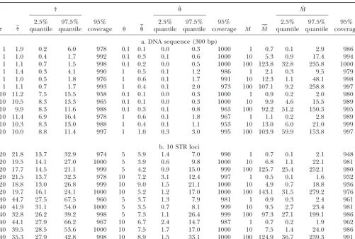
investigations have shown that with fewer (50,000)
simu-lations under the present model, the trend is similar to Parameter estimation from three demes :There are substantial gains in accuracy across a wide range of pa-that shown in Figure 1 as tolerance increased, but the
WED approach is considerably more accurate than the rameter value combinations when samples are drawn from three demes rather than from a single deme (Ta-standard method. For example, using the mtDNA
obser-vation set used above, and under identical conditions ble 2). For mtDNA sequences, expansion times are con-sistently estimated well and the range of estimates is except for a simulation size of 50,000, the RMSE forM
using P␦⫽0.01 for the standard ABC approach is 0.45 relatively narrow (Table 2a). The reduced coverage also implies that credible intervals of the posterior distribu-(⫾0.028 SE), which is substantially greater than that
from the WED modification (RMSE ⫽ 0.33 ⫾ 0.018 tions are narrower than that for 1-deme estimate while still encompassing the true parameter value inⵑ95% of SE). The greatest benefit of using the WED approach
thus accrues when the number of simulations is small cases. Migration estimates are also very accurate across the range of parameter combinations simulated. The range with respect to the number of parameters to be
esti-mated. All further estimation in this study was con- of estimates forMis relatively narrow and credible inter-vals show good coverage properties of the values under ducted using the WED modification.
The IE model was used to generate observation sets which the data sets were generated. Similarly,estimates are good with conservative credible intervals. Parame-under a range of known parameter values of ,, and
M. Analyses were conducted using samples from a single ters are also estimated well when using STR data (Table 2b). Expansion time estimates are consistently accurate, deme (deme 1) or from the three demes described
above. For each parameter combination, the behavior with a narrow range of estimates.Mestimates are now consistently good across the range of parameters simu-of the estimator was assessed using the mean and the
2.5 and 97.5 quantiles of the distribution of the 1000 lated, although with a tendency toward slight underesti-mation whenMis moderate. The 2.5 and 97.5 quantiles estimates, as well as the number of times the 95%
credi-ble intervals of the posterior distributions contained the show that the range of estimates of M is acceptable, and credible intervals of the posterior distribution show true parameter value (coverage property).
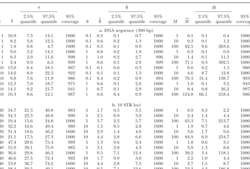
Parameter estimation from a single deme:When sam- good coverage of the true migration value with little substantial deviation from expectation. Population size ples are drawn from a single deme,FSTcannot be
calcu-lated, and it is therefore not used as a summary statistic. is also estimated well and does not show the tendency toward underestimation observed when data are sam-As reported in Table 1a for simulated DNA sequence
data, there is a substantial bias in estimates ofwhen pled from a single deme. However, the range of esti-mates of is broad for some parameter combinations expansion time is short and the scaled migration rate
Mis low to moderate. Estimates are more accurate un- when compared with the estimate range of other param-eters, and credible intervals are conservative.
der short expansion times when M increases, and the
range of estimates decreases as shown by the 2.5 and Application to the estimation of sex-biased dispersal in the common vole (M. arvalis):The present distribu-97.5 quantiles. Migration rate is underestimated when
expansion time is short and population size () is small. tional range ofM. arvalisspans most of Europe and the western parts of Asia (Mitchell-Joneset al.1999) and Again,andMare estimated quite well when migration
is large, and while the range of estimates foris good, Switzerland in the center of the Alps has been recently colonized after the melting of the ice cover ⵑ10,000 the 2.5 and 97.5 quantiles show that the distribution
of estimates for M is still very broad. Population size years ago. The mode of colonization and dispersal in small rodents suggests that the simple 2DSS world is an estimates were good across the set of parameter
combi-nations with an acceptable range. The coverage shows appropriate spatial model since physical restrictions and social association in subterranean burrows effectively that reconstructed 95% credible intervals were
TABLE 1
Range expansion parameters estimated from a single deme for samples of mtDNA sequences and 10 STR loci
ˆ ˆ Mˆ
2.5% 97.5% 95% 2.5% 97.5% 95% 2.5% 97.5% 95%
ˆ quantile quantile coverage ˆ quantile quantile coverage M Mˆ quantile quantile coverage
a. DNA sequence (300 bp)
1 10.9 7.3 14.1 1000 0.1 0.3 0.1 0.7 1000 1 0.1 0.1 0.4 1000
1 8.2 3.8 12.5 1000 0.1 0.6 0.2 1.3 1000 10 0.3 0.1 1.2 1000
1 1.8 0.8 4.7 1000 0.1 0.3 0.1 0.9 1000 100 62.5 0.6 263.6 1000
1 9.0 3.2 14.1 1000 1 0.8 0.2 1.9 1000 1 0.3 0.1 0.9 1000
1 6.3 2.0 11.6 999 1 1.0 0.2 2.7 996 10 1.4 0.1 11.5 1000
1 2.4 0.9 6.5 999 1 0.6 0.1 2.9 999 100 71.1 0.3 302.5 1000
10 13.0 8.4 18.5 967 0.1 0.1 0.0 0.3 1000 1 0.6 0.2 1.5 980
10 14.0 8.9 22.3 922 0.1 0.3 0.1 1.3 1000 10 4.6 0.7 12.8 1000
10 9.8 7.6 11.9 986 0.1 0.4 0.2 0.9 994 100 78.3 31.4 138.7 993
10 12.3 7.0 18.7 975 1 0.6 0.1 2.0 1000 1 1.0 0.1 3.2 943
10 14.1 9.2 21.7 941 1 0.7 0.1 2.9 1000 10 8.4 0.8 26.2 997
10 10.3 8.6 12.1 987 1 0.6 0.4 0.9 1000 100 124.8 66.1 218.4 986
b. 10 STR loci
20 34.7 21.3 49.8 983 5 1.7 0.5 3.5 1000 1 0.9 0.3 2.2 1000
20 34.3 22.3 48.8 999 5 2.1 0.9 3.9 1000 10 2.4 1.4 4.4 1000
20 19.4 15.6 24.8 1000 5 3.7 2.3 5.7 1000 100 65.3 7.1 213.7 1000
20 32.2 16.6 49.4 980 10 1.5 0.5 2.8 1000 1 1.9 0.7 4.6 1000
20 31.4 18.6 46.2 1000 10 2.9 1.4 4.9 1000 10 3.6 1.7 9.6 1000
20 21.1 17.5 27.3 1000 10 4.4 2.8 6.6 1000 100 84.9 6.9 254.7 1000
40 47.4 28.6 75.4 989 5 1.3 0.6 2.4 1000 1 1.8 0.6 3.1 1000
40 55.9 39.1 75.9 982 5 3.1 2.0 4.3 1000 10 3.9 1.3 8.6 1000
40 36.6 29.8 46.3 1000 5 9.5 7.1 12.4 1000 100 30.2 3.4 118.1 1000
40 46.6 27.5 72.4 992 10 1.7 0.9 3.0 1000 1 2.2 1.0 4.4 1000
40 53.8 36.7 74.2 1000 10 4.4 2.8 7.3 1000 10 3.7 1.5 8.7 1000
40 38.4 30.5 49.1 1000 10 9.5 7.1 12.6 1000 100 52.3 4.3 186.8 1000
Average estimations, 2.5 and 97.5 quantile values of the distributions of estimates from 1000 simulated samples are shown. “95% coverage” reports the number of simulated samples (among 1000) for which the true parameter lies within the 95% credible interval estimated from the posterior distribution.
toward males in Microtus like in the majority of mam- homogenous world, subject to the constraint that at least five nonsampled demes lay between each of the mals (Clutton-Brock1989;AarsandIms2000;
Clo-bertet al. 2001), but its effectiveness and the extent of sampling demes. Although sampling demes were as-signed to fixed positions during simulations, previous differences between the sexes are unknown since no
genetic studies have been conducted. We address these investigations have shown that the position of sampling sites has no discernible effect on estimated parameter questions forM. arvalisby analyzing a set of five
popula-tions (124 individuals) throughout Switzerland for values. For this, we created 12 simulation files (four replicates, with each replicate consisting of 3 simulation which data from 12 STR loci were typed and a 321-bp
fragment of the hypervariable region II of the mitochon- files). Within each replicate, sampling deme locations were fixed at randomly chosen positions; however, these drial control region was available (G. Heckel, R. Burri,
S. Fink, J.-F. Desmet and L. Excoffier, unpublished positions differed among replicates. All simulation files were challenged with the same observed data and esti-results). The five Swiss samples have been chosen
be-cause they present the same mtDNA (“central”) cytb mates of and M were made to assess whether the variation in estimates among replicates (due to sampling lineage, which is found in southern Germany and
north-ern Switzerland. We therefore assumed that the five deme position) was greater than variation within repli-cates. No such difference was found (data not shown). Swiss samples belonged to the same expansion wave that
has colonized Switzerland from the North after the last One million simulations were conducted for each type of molecular marker. Summary statistics for mtDNA glaciation (Fink et al. 2004). Simulations were
TABLE 2
Range expansion parameters estimated from three demes for samples of mtDNA sequences and 10 STR loci
ˆ ˆ Mˆ
2.5% 97.5% 95% 2.5% 97.5% 95% 2.5% 97.5% 95%
ˆ quantile quantile coverage ˆ quantile quantile coverage M Mˆ quantile quantile coverage
a. DNA sequence (300 bp)
1 1.9 0.2 6.0 978 0.1 0.1 0.0 0.3 1000 1 0.7 0.1 2.9 986
1 1.0 0.4 1.7 992 0.1 0.3 0.1 0.6 1000 10 5.3 0.9 17.4 994
1 1.1 0.7 1.5 998 0.1 0.2 0.0 0.5 1000 100 123.8 32.8 235.8 1000
1 1.4 0.3 4.1 990 1 0.5 0.1 1.2 986 1 2.1 0.3 9.5 979
1 1.0 0.5 1.8 976 1 0.6 0.1 1.7 991 10 12.3 1.1 48.1 998
1 1.1 0.7 1.7 993 1 0.4 0.1 2.0 973 100 107.1 9.2 258.8 997
10 11.2 7.5 15.5 958 0.1 0.1 0.0 0.3 1000 1 0.9 0.2 2.0 980
10 10.5 8.3 13.3 965 0.1 0.1 0.0 0.3 1000 10 9.9 4.6 15.5 989
10 9.9 8.3 11.6 988 0.1 0.3 0.1 0.8 963 100 92.2 51.2 150.3 995
10 11.4 6.9 16.4 978 1 0.6 0.1 1.8 967 1 1.1 0.2 2.8 989
10 10.3 8.3 13.0 988 1 0.4 0.1 1.1 953 10 13.0 6.0 21.0 999
10 10.0 8.8 11.4 997 1 1.0 0.3 3.0 995 100 103.9 59.9 153.8 997
b. 10 STR loci
20 21.8 13.7 32.9 974 5 3.9 1.4 7.0 990 1 0.7 0.1 2.1 948
20 19.5 14.1 27.0 1000 5 3.9 0.6 9.8 1000 10 6.8 1.1 22.1 981
20 17.7 14.5 21.1 999 5 4.2 0.9 15.0 999 100 125.7 25.4 252.1 980
20 21.5 13.7 32.3 978 10 7.2 3.1 12.4 997 1 0.5 0.1 1.6 932
20 18.8 13.0 26.8 999 10 9.0 1.5 21.1 1000 10 4.9 0.7 18.8 936
20 19.7 16.1 24.1 1000 10 5.2 1.2 17.0 1000 100 143.1 31.5 279.2 976
40 44.7 27.5 67.5 960 5 3.7 1.3 7.9 981 1 0.9 0.3 2.4 961
40 41.9 31.1 54.0 1000 5 3.5 0.7 8.1 999 10 9.5 2.7 23.4 981
40 32.8 26.2 39.2 998 5 7.3 1.1 26.4 999 100 97.3 27.1 199.1 986
40 44.1 27.9 66.2 967 10 6.7 2.4 14.7 987 1 0.7 0.2 1.9 962
40 39.5 28.5 53.6 1000 10 7.5 1.7 17.0 1000 10 7.5 1.4 24.0 986
40 35.3 27.9 42.8 998 10 8.9 1.5 33.1 1000 100 124.9 36.7 239.3 991
See Table 1 for details.
from prior distributions of-uniform [0:20],-log uni- mutation rate of 5 ⫻ 10⫺4 (Jarne andLagoda 1996; Ellegren 2004) and the reasonable assumption of form [0.01:20], andM-log uniform [0.01:500]. For STRs,
simulations were sampled from prior distributions of three generations per year (Hausser 1995), the time of the most recent range expansion was calculated as
-uniform [0:200],-log uniform [0.01:100], andM-log
uniform [0.01:500]. The ABC procedure was conducted ⵑ7667 years (with a 95% credible interval of 5455 to 11,337 years). For mtDNA,was estimated as 4.8 (Table as described previously. A tolerance of 0.001 was used for
each estimation procedure to give 1000 points for the 3). For the stretch of the control region used in this study, a mutation rate of 46% per site per million years of calculation of parameter estimates and the 95% credible
intervals of posterior distributions. The inferred scaled divergence was estimated by comparison with a related species with known divergence time (Finket al.2004), expansion time for STRs is 23.0 (Table 3). Using a STR
TABLE 3
Range expansion parameter estimates and the number of immigrant genes (Nm) per deme per
generation with 95% credible intervals (C.I.) for five vole populations in northern Switzerland, for samples of mtDNA sequences and STR loci
ˆ 95% C.I. ˆa 95% C.I. Mb 95% C.I. Nm 95% C.I.
mtDNA (321 bp) 4.8 2.8–8.0 1.8 0.1–6.1 0.29 0.02–2.5 0.15 0.01–1.25
STR (12 loci) 23 16.4–34 0.08 0.02–0.45 13.2 5.6–20.4 3.3 1.4–5.1
aestimates are presented for the whole chromosome rather than per site (base pair or STR locus). bMis equal to two times the number of immigrant females for mtDNA data, while it is equal to four times
explicit model using mtDNA sequences or STRs. The use of several summary statistics, each of which contains different information on the expansion process, allows for the simultaneous and accurate estimation of the time since the range expansion, the scaled population size, and the number of migrant genes exchanged be-tween neighboring demes. Furthermore, the introduc-tion of a weighted Euclidean distance giving greater weight to statistics that carry more information on a given parameter is shown to improve the accuracy of the estimation procedure, especially when the number of simulations is limited (Figure 1).
The ABC procedure is robust and estimates parame-ters consistently well across a broad range of parameter values in the two-dimensional stepping-stone model. A Figure2.—Plots of the posterior densities of the number
least-squares estimation procedure was proposed earlier
of immigrant genes (Nm) per deme per generation obtained
from the analysis of five northwestern Swiss vole populations. to estimate the parameters of a range expansion from The posterior density estimated using STRs is shown as a thin mismatch distributions computed from sequence data line, the posterior density estimated using mtDNA is shown
under an infinite island model (Excoffier2004).
Simu-as a thick line, and the estimated posterior density of the
lations have shown that this method provides reasonable
males obtained as a convolution of mtDNA and STR densities
estimates of, but it was found to be highly unreliable
is shown as a dashed line.
for estimating the migration parameter M (data not shown), because the mismatch distribution has a high although this estimate may be conservative due to the associated variance for lowM-values and is uninforma-potential for multiple hits per site. By again assuming tive forMwhen this parameter is large (M⬎50) ( Excof-three generations per year, the inferred expansion time fier2004). The ability to use other aspects of molecular for mtDNA isⵑ8127 years (with a 95% credible interval diversity, both within and between demes, considerably of 4725–13,605 years), showing that the two types of improves the estimation of the migration parameter, markers are in excellent agreement in showing a post- such that reliable estimates of sex-specific dispersal are glacial colonization time of Switzerland. As expected, possible.
estimation of theMparameter differs significantly be- As shown above, the accuracy of the estimation in-tween mtDNA and STR data (Table 3), withMSTR⫽13.2 creased when more demes were sampled. While
sam-(95% credible interval [5.6, 20.4]) for nuclear genes and pling from a single deme provided satisfactory estimates
Mmt ⫽ 0.29 [0.02, 2.5] for mtDNA. The difference in for some parameter combinations, it resulted in poor
ploidy and transmission pattern between mtDNA and estimates for other combinations, particularly when STR markers implies thatMSTR⫽4Nem, whereNeis the expansion times were short and migration was low. The
effective population size andNemis the effective number improvement due to the use of several demes is linked
of nuclear genes (3.3) exchanged between neighboring to the additional information available, but also to the demes per generation, whileMmt⫽2Nfm, whereNfis fact that when the total number of demes in the
popula-the number of females andNfmis the number of female tion is large, the gene genealogies of different samples
genes (0.145) exchanged between demes per genera- are almost independent after the expansion, thus pro-tion. The posterior distribution of the Nm values for viding replicate information on the migration process female, male, and total immigrant genes is shown in between neighboring demes. Moreover, information on Figure 2. The male posterior distribution was obtained the amount of differences between demes can be incor-from the convolution of the total and female densities, porated, for instance, by using the FST statistic, while
under the simple assumption thatNe⫽Nm⫹Nf. The only within-deme diversity can be used with a single
inferred male density has a mode at Nm ⫽ 3.01 and deme. It should be noted, however, that using informa-limits of an equal-tail 95% credible interval at 1.31 and tion from several demes to estimate a migration parame-5.2. Since the ratio of point estimates for male and ter assumes that it is a parameter tied to the biology femaleNmvalues is 20.76, it suggests that males move of the species rather than being location specific and
ⵑ20 times more than females, in agreement with an postulates that dispersal patterns will be equivalent at
extreme philopatry of females. different locations. In that sense the different samples
can be considered as replicates of the same process. This assumption is likely to be reasonable when samples
DISCUSSION
are drawn from similar environments. Additionally, the use of several demes in a single estimation procedure The results presented here show that ABC can be
wave. Obviously, our results could be erroneous if a deme size, the number of immigrants (Nm) estimated for males and females may not necessarily apply to the species had occupied its present range by a series of
independent range expansions (i.e., from different ref- same spatial scale. The 20-fold larger rate of immigra-tion for males compared to female voles could thus uge areas) and if sampled demes were drawn from
re-gions colonized from different sources. be an overestimation if the males were dispersing over
larger distances than the females. We nevertheless show An attractive feature of the ABC method is its ability
to handle different types of molecular markers easily, here how information on nuclear and mtDNA markers can be combined to get estimates of male dispersal, such as DNA sequences or microsatellites, but SNP data
could also be used if possible sources of ascertainment without the need for male-specific markers.
While our study suggests that the ABC procedure is bias could be simulated (e.g.,Wakeleyet al. 2001). One
particularly useful application is therefore to compare an efficient means of estimating parameters in the 2DSS model, more refined spatial models could be consid-parameter estimates obtained from different markers,
to assess either similarities or any discrepancies that ered, which could include a number of realistic features such as coastlines or environmental heterogeneity that may carry valuable biological information. There is a
remarkable concordance in expansion time estimates are likely to be important in shaping the molecular diversity of expanding populations. A simulation model inferred from mtDNA and STRs for the common vole
in Switzerland. These estimates are highly plausible that can include these factors as well as a more progres-sive range expansion has been recently made available since this suggests the onset of the range expansion
occurred after most of the ice cap covering the region (SPLATCHE,Curratet al.2004). Because simulations under this model are considerably slower than those during the last glacial maximum had melted by 12,000
years before present and the glaciers had retreated to reported here, its coupling to the ABC procedure is currently difficult, but should be possible with forthcom-the highlands (Hewitt1999). Moreover, from the
rela-tively extensive simulation studies on the performance ing increases in computing power. Since the accuracy of the ABC procedure depends in part on the number of our methodology reported in Tables 1 and 2, we see
that the coverage property of the posterior distributions of simulations used (and hence on simulation time), one interesting challenge for the future will be to deter-is conservative with 1 million simulations and a tolerance
level of 0.1%, so that we are confident that the estima- mine the benefits of increased model complexity and realism,vs.simulation size. Compared to likelihood ap-tions obtained from the vole data using the same
num-ber of simulations and tolerance level are valid. The proaches, the ABC methodology is much easier to imple-ment for complex demographic models, but it does not existence of glaciation data external to the genetic data
is extremely useful to further validate the expansion use as much data and should thus not be expected to be as accurate. A potential difficulty of the ABC ap-time estimates. Therefore, the good agreement between
these independent data sources suggests that the ABC proaches is in the choice of summary statistics and in the definition of the appropriate tolerance level, which method may work well when such corroborative data are
not available. In contrast to the similarity in estimated are difficult to assessa priori. Therefore, simulation stud-ies on the performance of the methodology should be expansion times for Northern Swiss vole mtDNA
se-quences and STRs, migration estimates showed an ex- conducted before applying it to observed data, to check for potential biases and for good coverage properties treme sex bias in dispersal, with males dispersing atⵑ20
times the rate of females. This extreme difference in of posterior distributions. Overall, however, this study shows that the ABC procedure should provide a valuable the immigration rate between the sexes was unexpected,
although the direction of the bias is completely in agree- and flexible tool for investigating questions involving range expansions, including those related to sex-biased ment with observational data (Clutton-Brock 1989;
Aars and Ims 2000; Clobert et al.2001; G. Heckel, dispersal or to the history of human settlement. unpublished data). Note here that our estimates reflect We are grateful to Pierre Berthier and Samuel Neuenschwander the effective number of immigrants received by each for computing assistance, to Sabine Fink and Reto Burri for assistance in the laboratory, and to Arnaud Estoup for helpful comments on
deme from surrounding unsampled subpopulations
the manuscript. This work was supported by a Swiss National Science
and not the number of genes exchanged between
sam-Foundation grant no. 3100A0-100800 to L.E.
pled demes, which is in clear contrast with other meth-ods aiming at estimating migration rates (e.g., Beerli
andFelsenstein2001). However, since the 2DSS model
LITERATURE CITED
is an approximation of a more continuous distribution
Aars, J., andR. A. Ims, 2000 Population dynamic and genetic
conse-of individuals (Bartonand Wilson 1995), the exact
quences of spatial density-dependent dispersal in patchy
popula-delineation of a deme and its neighborhood size should tions. Am. Nat.155:252–265.
Barton, N. H., andI. Wilson, 1995 Genealogies and geography.
depend on the pattern of the dispersal distance of
indi-Philos. Trans. R. Soc. Lond. Ser. B349:49–59.
viduals, which may not be identical for males and
fe-Beaumont, M. A., 1999 Detecting population expansion and decline
males. In that case, because we expect a quadratic rela- using microsatellites. Genetics153:2013–2029.
Beaumont, M. A., W. ZhangandD. Balding, 2002 Approximate
Bayesian computation in population genetics. Genetics 162: Goldstein, D. B., G. W Roemer, D. A. Smith, D. E. Reich, A.
Berg-2025–2035. man et al., 1999 The use of microsatellite variation to infer
Beerli, P., andJ. Felsenstein, 2001 Maximum likelihood estima- population structure and demographic history in a natural model
tion of a migration matrix and effective population size in n system. Genetics151:797–801.
subpopulations by using a coalescent approach. Proc. Natl. Acad. Hausser, J.,1995 Sa¨ugetiere der Schweiz: Verbreitung, Biologie, Oekologie. Sci. USA98:4563–4568. BirkHa¨user Verlag, Basel, Switzerland.
Currat, M., N. RayandL. Excoffier, 2004 SPLATCHE: a program Hewitt, G. M., 1999 Post-glacial re-colonization of European biota.
to simulate genetic diversity taking into account environmental Biol. J. Linn. Soc.68:87–112.
heterogeneity. Mol. Ecol. Notes4:139–142. Hewitt, G. M., 2000 The genetic legacy of the Quaternary ice ages.
Clobert, J., E. Danchin, A. A. DhondtandJ. D. Nichols, 2001 Nature405:907–913.
Dispersal. Oxford University Press, Oxford. Jarne, P., andP. J. L. Lagoda, 1996 Microsatellites, from molecules
Clutton-Brock, T. H., 1989 Mammalian mating systems. Proc. R. to populations and back. Trends Ecol. Evol.11:424–429.
Soc. Lond. Ser. B236:339–372. Mitchell-Jones, A. J., G. Amori, W. Bogdanowicz, B. Krystufek,
Ellegren, H., 2004 Microsatellites: simple sequences with complex P. J. H. Reinjnderset al., 1999 The Atlas of European Mammals.
evolution. Nat. Rev. Genet.5:435–445. T. & A. D. Poyser, London.
Estoup, A., andS. M. Clegg, 2003 Bayesian inferences on the recent Nielsen, R., andJ. Wakeley, 2001 Distinguishing migration from
island colonization history by the birdZosterops lateralis lateralis. isolation: a Markov chain Monte Carlo approach. Genetics158:
Mol. Ecol.12:657–674. 885–896.
Estoup, A., I. J. Wilson, C. Sullivan, J. M. CornuetandC. Moritz, Pritchard, J. K., M. T. Seielstad, A. Perez-Lezaunand M. W.
2001 Inferring population history from microsatellite and
en-Feldman, 1999 Population growth of human Y chromosomes:
zyme data in serially introduced cane toadsBufo marinus.Genetics a study of Y chromosome microsatellites. Mol. Biol. Evol. 16:
159:1671–1687.
1791–1798.
Estoup, A., M. Beaumont, F. Sennedot, C. MoritzandJ.-M.
Cor-Ray, N., M. CurratandL. Excoffier, 2003 Intra-deme molecular
nuet, 2004 Genetic analysis of complex demographic scenarios:
diversity in spatially expanding populations. Mol. Biol. Evol.20:
spatially expanding populations of the cane toad,Bufo marinus.
76–86. Evolution58:2021–2036.
Tavare´, S., D. J. Balding, R. C. GriffithsandP. Donnely, 1997
Excoffier, L., 2004 Patterns of DNA sequence diversity and genetic
Inferring coalescence times from DNA sequence data. Genetics structure after a range expansion: lessons from the infinite-island
145:505–518. model. Mol. Ecol.13:853–864.
Wakeley, J., R. Nielsen, S. N. Liu-CorderoandK. Ardlie, 2001 The
Fink, S., L. ExcoffierandG. Heckel, 2004 Mitochondrial gene
discovery of single-nucleotide polymorphisms—and inferences diversity in the common voleMicrotus arvalisshaped by historical
about human demographic history. Am. J. Hum. Genet.69:1332– divergence and local adaptations. Mol. Ecol.13:3501–3514.
1347.
Fu, Y. X.,andR. Chakraborty, 1998 Simultaneous estimation of
Wang, J., andM. C. Whitlock, 2003 Estimating effective population
all the parameters of a stepwise mutation model. Genetics150:
size and migration rates from genetic samples over space and 487–497.
time. Genetics163:429–446.
Fu, Y. X., andW. H. Li, 1997 Estimating the age of the common
ancestor of a sample of DNA sequences. Mol. Biol. Evol. 14: