Bayesian Mapping of Quantitative Trait Loci Under Complicated Mating Designs

Copyright2001 by the Genetics Society of America

Bayesian Mapping of Quantitative Trait Loci Under Complicated Mating Designs

Nengjun Yi and Shizhong Xu

Department of Botany and Plant Sciences, University of California, Riverside, California 92521

Manuscript received April 10, 2000 Accepted for publication December 19, 2000

ABSTRACT

Quantitative trait loci (QTL) are easily studied in a biallelic system. Such a system requires the cross of two inbred lines presumably fixed for alternative alleles of the QTL. However, development of inbred lines can be time consuming and cost ineffective for species with long generation intervals and severe inbreeding depression. In addition, restriction of the investigation to a biallelic system can sometimes be misleading because many potentially important allelic interactions do not have a chance to express and thus fail to be detected. A complicated mating design involving multiple alleles mimics the actual breeding system. However, it is difficult to develop the statistical model and algorithm using the classical maximum-likelihood method. In this study, we investigate the application of a Bayesian method implemented via the Markov chain Monte Carlo (MCMC) algorithm to QTL mapping under arbitrarily complicated mating designs. We develop the method under a mixed-model framework where the genetic values of founder alleles are treated as random and the nongenetic effects are treated as fixed. With the MCMC algorithm, we first draw the gene flows from the founders to the descendants for each QTL and then draw samples of the genetic parameters. Finally, we are able to simultaneously infer the posterior distribution of the number, the additive and dominance variances, and the chromosomal locations of all identified QTL.

T

HE availability of dense molecular marker maps Slate et al. 1999). The main reasons behind this

in-creased power are: (1) a complex pedigree increases provides a large opportunity to locate genes

respon-sible for variation of quantitative traits in plants, animals, the chance that founder alleles are equally represented in the mapping population; and (2) there are more and humans. Experimental design and methodology

are two important issues in quantitative trait loci (QTL) informative meioses in a complex pedigree than in a simple pedigree for the same number of genotypes. mapping. Most QTL mapping techniques require

de-signed line crosses, e.g., F2 or backcross (BC). These A variety of methods have been developed for QTL

mapping (Hoeschele at al.1997; Lynchand Walsh

crosses do not exist in natural populations and are not

1998). These methods can be classified into three cate-commonly used in some plant species in the breeding

gories: least-squares analysis (LS), maximum-likelihood industry. It is not economical to design such line cross

analysis (ML), and Bayesian analysis. These methods experiments solely for the purpose of QTL mapping if

differ in computational requirement, efficiency in terms these crosses are not regularly used in a breeding

pro-of extracting information, flexibility with regard to han-gram. Almost all natural populations and most

domesti-dling different data structures, and ability in mapping cated plant populations consist of complicated pedigree

multiple QTL. The simple LS method is efficient in structures. Even if inbred lines are used, different

terms of computational speed, but cannot extract all crosses may be connected by some common ancestors.

information from the data and is restricted to specific A mating design combining information from multiple

mating designs. ML interval mapping (Lander and

crosses is more powerful than one involving a single

Botstein1989) is one of the most widely used methods cross (Muranty 1996;Xu 1998). Multiple crosses

in-for QTL analysis in a single cross. The interval mapping crease the polymorphic levels of QTL alleles and may

method has been extended to composite interval map-permit the detection of QTL that are undetectable in

ping and multiple interval mapping (Jansen1993;Zeng

a single line cross. Animal and human geneticists have

1993;Kaoet al. 1999). These extensions are designed paid considerable attention to the relative power of

particularly for mapping multiple QTL in a single line simple pedigree analysis and more complicated family

cross. However, it is not straightforward to apply these structures in linkage analysis of QTL and found that

methods to QTL mapping in general pedigrees. The large complex pedigree designs are usually more

power-identical-by-descent-based variance component method ful (e.g.,Welleret al.1990;WijsmanandAmos1997;

can be applied to general pedigrees (Almasy and

Blangero 1998). This method not only incorporates full pedigree information but also is robust to the num-Corresponding author:Shizhong Xu, Department of Botany and Plant

ber of QTL alleles. In addition, it does not require the

Sciences, University of California, Riverside, CA 92521.

E-mail: [email protected] knowledge of marker linkage phases (Schork 1993;

Amos 1994;XuandAtchley1995). The identical-by- reversible jump Markov chain Monte Carlo (MCMC) algorithm, which allows simultaneous estimation of the descent (IBD)-based variance component approach has

become a very useful strategy for QTL mapping in hu- number, the locations, and effects of identified QTL.

mans. If the linkage phase information is indeed known, by ignoring such information, the IBD method may be

STATISTICAL METHODS suboptimal. It is also questionable to apply this method

to plants where the pedigree sizes are usually large due Mixed model:Assume that the mapping population

to the need to invert large IBD matrices repeatedly for consists ofnindividuals with arbitrary pedigree

relation-each QTL position considered. ships, and among thenindividuals there aremfounders

Bayesian analysis is preferable because of its conve- and (n⫺m) nonfounders. The whole population may

nience and flexibility in the use of full pedigrees and consist of a single large pedigree or multiple

indepen-mapping multiple QTL, although it is computationally dent pedigrees. A founder in a pedigree is defined as

very demanding. Bayesian mapping fully takes into ac- an individual with no parents included in the pedigree. count the uncertainties associated with all unknowns in In contrast, a nonfounder is defined as an individual

the QTL mapping problem, including the number and with both parents included in the pedigree. Founders

locations of QTL, effects of QTL, and the genotypes of are assumed to be unrelated but can be inbred. The

markers and QTL. In plant line-crossing experiments, descendants may be related in an arbitrary way.

Bayesian mapping has been developed by using the Let y represent an n ⫻ 1 vector for the observed

Markov chain Monte Carlo algorithm, in particular, for values of a quantitative trait. When the trait is controlled

detection of multiple QTL (Satagopanand Yandell by multiple genes acting independently, y can be

de-1996;Satagopanet al.1996;Sillanpa¨a¨andArjas1998, scribed by the linear model

1999;Stephens andFisch1998;Yi andXu2000). In

y⫽Xb⫹

兺

l

j⫽1

(up

j ⫹umj ⫹ vj)⫹ e, (1)

animals and humans, Bayesian mapping has been de-signed not only to map multiple QTL, but also to extract

full pedigree information (Heath 1997; Uimari and whereXis a known design matrix for a vector of

nonge-Hoeschele 1997). However, most existing Bayesian netic effects b (including the overall mean), l is the

mapping methods assume a biallelic QTL model. Al- number of QTL on all chromosomes,up

j andumj aren⫻

though this assumption may be reasonable for a single 1 vectors for the paternal and maternal allelic effects line cross, it is less so for complex pedigrees. Therefore, for thejth QTL,vjis ann⫻1 vector for the dominance

Bayesian mapping needs to be extended to multiallelic effects for thejth QTL, ande is the vector of residual

systems. (environmental) effects. This model is written in the

There are several differences between plants and ani- original form of the animal model (Fernando and

mals or humans in the context of general pedigrees: Grossman1989) except that we have included the

dom-(i) many plant species are self-compatible and one must inance effects.

deal with a system that involves a mixture of selfing Denote aj as a 2m⫻ 1 vector for the effects of the

and outcrossing; (ii) inbreeding and line crossing are founder alleles (withmancestors, each with two alleles)

common mating designs in most plant breeding popula- and dj as a vector of interaction effects (dominance

tions; (iii) a breeding population of plants usually con- effects) between all possible pairs of the 2m founder tains fewer founders than an animal or human popula- alleles at thejth QTL. The dimension ofdjism(2m⫹

tion and the founders can be pure inbred lines; and 1). The dimension ofdjcan be reduced greatly in some

(iv) family sizes of plants are usually large compared mating designs where it is impossible for some founder

with animals and humans. These differences provide alleles to be combined in any descendant. The QTL

additional opportunities for detecting QTL. Unfortu- effects of all individuals can be expressed as linear func-nately, the Bayesian mapping methods developed for tions of the allelic effects and their interactions in the human and animal pedigrees cannot handle the unique founders,i.e.,up

j ⫽Zpjaj,umj ⫽Zmjaj, andvj⫽Wjdj, leading

properties for plant pedigrees. This poses unique chal- to

lenges for plant geneticists to develop new QTL

map-y⫽ Xb⫹

兺

l

j⫽1

(Zp

j ⫹ Zmj)aj⫹

兺

l

j⫽1

Wjdj⫹e. (2)

ping statistics.

In this article, we develop a Bayesian method of QTL

mapping under arbitrarily complicated mating designs, This model is written in the form of a reduced animal

model (CantetandSmith1991) in which each allele

including a group of independent or related F2or

back-cross populations and complicated multiple-generation is traced back to one of the founder alleles throughn⫻

2mmatricesZp

j andZmj, also called the allelic inheritance

cross populations derived from inbred or outbred

founders. The method is so flexible that it can handle matrices. Note that the n ⫻ m(2m ⫹ 1) dominance

design matrixWjis a function ofZpj andZmj. The allelic

a variety of genetic models, such as arbitrary number of

the chromosome on which thejth QTL resides. There- each QTL has a uniform distribution of residing at any location on that chromosome. The prior distributions fore, the distributions of Zp

j and Zmj are functions of

marker information and the chromosomal location of of band␴2

eare assumed to be uniform on predefined

intervals, although other priors can be used. Finally, thejth QTL. The environmental effects are assumed to

follow aN(0,I␴2

e) distribution. p(Zp,Zm,M|l,␭,M*) is the joint conditional distribution

of QTL allelic inheritance matrices and complete The observables in model (2) include the phenotypic

values,y⫽{yi}ni⫽1, the covariateX, and the marker data marker genotypes.

In some situations, we need to add an extra layer to

M*. The marker data include the locations of markers

on chromosomes and the observed (possibly incom- the hierarchical model. The distributionsp(aj) andp(dj)

depend on other unknown quantities␴2

aj and ␴ 2 dj, the

plete) marker genotypes. The observed marker

geno-types in some individuals may not be fully informative allelic and dominance variance of thejth QTL. In other words, we replacep(aj) byp(aj,␴2aj)⫽ p(aj|␴

2 aj)p(␴

2 aj) and

and the patterns of allelic inheritance of such markers

p(dj) by p(dj,␴2dj)⫽p(dj|␴ 2 dj)p(␴

2

dj). The parameters of

may also be unknown. The list of unobservables includes

interest now are␴2 ajand␴

2

dj, withajanddjbeing treated

the number of QTLl, the QTL locations␭⫽{␭j}lj⫽1, the

as missing values. The joint posterior distribution of all

complete marker genotype matrixM, the QTL allelic

variables is then factorized as inheritance matricesZp⫽ _{Zp

j}lj⫽1 andZm⫽ {Zmj}lj⫽1, the

QTL allelic effectsa ⫽{aj}lj⫽1, the QTL dominance

ef-p(␪,Va,Vd|y,X,M*)⬀p(y|␪)p(Zp,Zm,M|l,␭,M*)

fectsd⫽{dj}lj⫽1, and the residual variance␴2e. The

loca-tion parameter,␭j, is expressed as the distance of thejth ⫻p(l)p(b)p(␴2e)

QTL from one end of the chromosome. The complete

⫻

兿

l j⫽1

兵

p(aj|␴2 aj)p(␴

2 aj)p(dj|␴

2 dj)

marker genotype means marker genotype with known linkage phase. A complete genotype for a nonfounder

⫻p(␴2

dj)p(␭j)

其

, (5)

means a known allelic inheritance pattern. The QTL dominance design matrices are suppressed in the list

where Va ⫽ {␴2aj} l

j⫽1,Vd⫽ {␴2dj} l

j⫽1, and the distributions

of unknowns because they are completely determined

p(aj|␴a2j) and p(dj|␴ 2

dj) are multivariate normal as given

by the QTL allelic inheritance matrices.

in the appendix. We use uniform prior distributions

In a Bayesian framework, the unknowns in the model

forp(␴2

aj) and p(␴ 2

dj) within some predetermined

inter-are considered to be drawn from appropriate prior

dis-vals. Other terms in Equation 5 are the same as in tributions. The joint posterior distribution of all

unob-Equation 3. servables ␪ ⫽ {l, ␭, a, d, b, M, Zp_{, Z}m_, ␴2

e} given the

Equations 3 and 5 correspond to two different ap-observables {y, X, M*} and prior information can be

proaches in QTL mapping, i.e., the fixed-model and

expressed as

the random-model approaches, respectively. If there are only a few founders who are not randomly sampled

p(␪|y,X,M*)⬀p(y|␪)p(Zp_,Zm_,M|_l,␭_,M*)

from a large reference population, our interest may be ⫻p(l)p(b)p(␴2

e)

only in the values of the actual allelic effects and the dominance effects for the founders at hand. Under the ⫻

_兿

l

j⫽1

兵

p(aj)p(dj)p(␭j)

其

. (3)

fixed-model approach the priors for the allelic and dom-inance effects are treated as variable with known distri-The likelihood functionp(y|␪) depends on the

distri-butions. The fixed-model approach is very common in bution of y. For normally distributed traits, it has the

designed line-crossing experiments,e.g., F2and BC

de-form _{signs, where the average effect of allelic substitution}

is the parameter of interest. When the founders are

p(y|␪)⬀(␴2

e)⫺n/2⫻ exp

冦

⫺

1 2␴2

e

RT_R

冧

_{, (4)}

randomly sampled from a reference population, we are usually interested in the variances of the genetic effects in the population from which the founders are sampled.

whereR⫽ y⫺Xb⫺Rl

j⫽1(Zpj ⫹Zmj)aj⫺Rlj⫽1Wjdj.

The priors of the allelic and dominance effects of In this case, the distributions for the allelic and domi-nance effects of founders depend on some unknown QTL,p(aj) andp(dj), depend on the inbreeding

coeffi-cients of the founders (seeappendix). The inclusion parameters. When the number of founders is so small

that a meaningful estimate of the allelic or dominance of inbreeding coefficients of founders enables the

pro-posed method to treat inbred founders. The prior distri- variance cannot be inferred from the limited number of alleles sampled, we may still use the fixed-model ap-bution of the number of QTL,p(l), is assumed to be

a truncated Poisson distribution with mean ␮ and a proach, even if the founders are a random sample. In

this study, we concentrate on the random model

ap-predefined maximum numberlmax. When no

informa-tion regarding the locainforma-tions is available, the prior proba- proach.

Reversible jump MCMC: In Bayesian analysis, infer-bility that a QTL is on a chromosome is proportional to

joint posterior distribution of all unknowns. Since the where ␪* means all elements of ␪ except thataj kis

re-placed by the proposalaj* k .

joint posterior distribution does not have a standard

The dominance effects of QTL are updated for two form, MCMC samplers are used to generate samples

founders at a time, again in a locus-by-locus basis. De-from the joint posterior distribution (Metropoliset al.

notedj

kk⬘as a vector of dominance effects between alleles

1953;Hastings1970;GemanandGeman1984;Green

of founderkand alleles of founder k⬘at the jth QTL. 1995). The MCMC algorithm consists of the following

The dimension of dj

kk⬘ is three or four, depending on

steps:

whether k equals k⬘ (see the appendix). To update

a. Updating QTL allelic effectsa⫽ {aj}lj⫽1; _dj_{kk⬘, a new proposal d}j_kk*_{⬘ is simulated by random walk,}

b. Updating QTL dominance effects d⫽{dj}lj⫽1; _{denoted by}

c. Updating QTL allelic variancesVa⫽ {␴2aj} l j⫽1;

dj*

kk⬘⫽ djkk⬘⫹(␦1,fk␦1⫹(1⫺ fk)␦2,fk␦1⫹ (1⫺fk)␦4)T

d. Updating QTL dominance variancesVd⫽ {␴2dj} l j⫽1;

e. Updating the fixed effects b and residual variance

ifk⬘ ⫽k; otherwise, ␴2

e;

f. Updating complete marker genotypes M and QTL dj*

kk⬘⫽ djkk⬘⫹(␦1,fk␦1⫹(1⫺ fk)␦2,fk⬘␦1

allelic inheritance matricesZp_andZm_;

⫹(1⫺ fk⬘)␦3,fkfk⬘␦1⫹ (1⫺fk)fk⬘␦2

g. Updating QTL locations␭⫽ {␭j}lj⫽1;

⫹fk(1⫺fk⬘)␦3⫹(1⫺ fk)(1⫺ fk⬘)␦4)T,

h. Birth of a QTL (adding one new QTL to the model) or death of a QTL (removing one existing QTL from

where␦1,␦2,␦3, and␦4are sampled independently from

the model).

the symmetric uniform distribution around zero. The new proposal is accepted with probability

The proposed algorithm starts from an initial point and proceeds to update each of the unknowns in turn.

min

冦

1,p(y|␪*)p(d

j* kk⬘|␴d2j)

p(y|␪)p(dj kk⬘|␴2dj)

冧

, (7)

One complete pass over these eight update steps defines a cycle of iteration. Updating steps (a)–(g) are

conven-tional and do not alter the dimension of the variable _{where ␪* means all elements of ␪ except that d}j

kk⬘ is

vector. We use Metropolis-Hastings algorithms to imple- _{replaced by the proposald}j* kk⬘.

ment steps (a)–(e) and (g), and the Gibbs sampler to _{Updating QTL variances: QTL allelic and dominance}

update step (f). Step (h) involves changing QTL num- _{variances are updated locus by locus. To update␴}2 ajand

ber by one and making necessary corresponding _␴2

dj, new proposals ␴2*aj and ␴2*dj are sampled from the

changes to (a, d, Va,Vd, Zp, Zm, ␭). A reversible jump _{symmetric uniform densities around their previous}

val-step is needed to change the number of QTL.

ues. The proposals are accepted with probabilities Several methods have been available for updating

marker genotypes in general pedigrees (e.g.,Sobeland

Lange 1996; Heath 1997; Uimari and Hoeschele _min

冦

_1,

兿

km⫽1p(ajk|␴2*a_j)

兿

m

k⫽1p(ajk|␴2a_j)

冧

and min

冦

1,

兿

m

k⫽1

兿

mk⬘⫽kp(djkk⬘|␴2*d_j)

兿

m

k⫽1

兿

m

k⬘⫽kp(djkk⬘|␴2d_j)

冧

, 1997;BinkandVan Arendonk1999). In the simulation

study (see the next section), we adopt the method of ₍₈₎

BinkandVan Arendonk(1999) to update the marker

respectively. genotypes. For more complicated situations, a descent

Updating QTL allelic inheritanceZp_andZm_{:Each allele}

graph sampler of Sobel andLange (1996) is needed

in the descendants can be traced back to one of the (seediscussion). Updating the fixed effectsband

resid-founder alleles. This is reflected byap

j ⫽Zpjajandamj ⫽

ual variance␴2

eis also straightforward.

Zm

jaj, where each row of matrices Zpj and Zmj has one Updating QTL effects: The allelic effects of QTL are

element taking 1 and all other elements being 0. It is updated founder by founder and locus by locus. Denote

not convenient to generate realizations of Zp

j and Zmj aj

k as a 2 ⫻ 1 vector for the allelic effects of the kth

directly, but we can easily generate a sample ofZp j and

founder at thejth QTL (appendix). To updateaj k, two

Zm

j indirectly through the following recursive approach.

random variables, ␦1 and ␦2, are simulated

indepen-Consider a pedigree with m founders. Let the 2m

dently from the symmetric uniform distribution around

founder alleles be numbered consecutively from 1 to zero (random walk). The length of this uniform

distribu-2m.Then allele 2k⫺1 and 2kare the two alleles of the tion is determined empirically and should result in a

kth founder. Assume that individuals are entered into reasonable rate of average acceptance rate. A new

pro-the pedigree in a chronological order so that pro-the parents posal value ofaj

ktakesajk*⫽ajk⫹(␦1,fk␦1⫹(1⫺fk)␦2)T,

are evaluated before their progeny. Denote Zp j(i) and

wherefkis the inbreeding coefficient of thekth founder.

Zm

j(i) as theith rows of Zpj andZmj, respectively;i.e.,Zpj

The new proposal is accepted with probability

(i) andZm

j(i) store the allele identifications of the

pater-nal and materpater-nal alleles of individuali, respectively. For min

冦

1,p(y|␪*)p(a

j* k|␴2aj)

p(y|␪)p(ajk|␴2 aj)

冧

, (6)

back to allele 3 of the founders and the maternal allele The proposals are accepted with probability is traced back to allele 10 of the founders, then the

third element ofZp

j(i) is 1 and all other elements are _min 1,

p(y|␪*,␭*j,Zpj*,Zmj*)

p(y|␪) ⫻ p(Up*

j ,Umj*|␭j*,GLj,GRj)

p(Up

j,Umj|␭j,GLj,GRj)

⫻ q(Upj,Umj)

q(Up*

j,Umj*)

  ,

0, and the tenth element of Zm

j(i) is 1 and all other

(9) elements are 0. We now describe the recurrent process

of building matrices Zp

j and Zmj. Assume that we have

where ␪* contains all elements of ␪ except ␭j, Zp j, Zmj.

already built matricesZp

j andZmj up to the first (i⫺1)th

LetGL

j(GRj) denote the complete genotypes of all

pedi-rows and are ready to build the ith rows. If the ith

gree members at the left (right) flanking locus of the individual is a founder, say thekth founder, then the

corresponding location. If the proposals are accepted, (2k⫺1)th element ofZp

j(i) and the (2k⫹1)th element

we update the location of thejth QTL and also modify ofZm

j(i) are 1. If theith individual is not a founder but

the segregation indicators, the allelic inheritance, and the progeny of individualsi1 (father) andi2(mother),

dominance design matrices at thejth QTL at the same then

time.

Updating QTL number:The reversible jump mechanism

Zp

j(i) ⫽upijZpj(il)⫹(1⫺ upij)Zmj(i1)

is needed to change the QTL number in the model. In

and _{this study, a reversible pair is used: birth/death of a}

QTL. In every cycle of the simulation, we make a random

Zm

j(i)⫽ umijZpj(i2)⫹ (1⫺umij)Zmj(i2),

choice between attempting to add one new QTL into the model or delete one existing QTL from the model, whereup

ijandumij are the paternal and maternal

segrega-with probabilities pa andpd ⫽ 1 ⫺ pa, respectively. Of

tion (meiosis) indicators, respectively, for individual i

course,pa⫽0 ifl⫽lmaxandpd⫽0 ifl⫽0, and otherwise

at the jth QTL. If the paternal allele of the father is

we choosepa⫽0.5, for 0⬍l⬍ lmax.

passed to individuali, thenup

ij⫽ 1; otherwise,upij⫽ 0.

For a birth step, we need to generate a new location The value ofum

ij is similarly defined but for the allelic

␭l⫹1, a new allelic variance␴2al⫹1, a new dominance

vari-inheritance of the mother. Note that Zp

j(i1),Zmj(i1),

ance␴2

dl⫹1, a new vector of allelic effects of the founder

Zp

j(i2), and Zmj(i2) have been previously built because

allelesal⫹1, a new vector of dominance effects between i1ⱕi⫺1 andi2ⱕi⫺1. Therefore, to trace the allelic

all possible pairs of the founder alleles dl⫹1, and new

origin, one only needs to simulate the segregation

indi-inheritance and dominance design matrices of all pedi-cators for each descendant.

gree membersZp

l⫹1,Zml⫹1, andWl⫹1for the new QTL. The

Simulating the segregation indicators (up

ij, umij) is

new location ␭l⫹1 and the variances ␴2al⫹1 and ␴ 2 dl⫹1

straightforward. The segregation indicators (up

ij,umij) can

are sampled from the corresponding prior densities. take four possible values,i.e., (1, 1), (1, 0), (0, 1), and

The allelic effects al⫹1 and the dominance effects dl⫹1

(0, 0). The conditional posterior distribution is thus a

are then simulated from the distributionsp(al⫹1|␴2a_l⫹1)

discrete distribution over the four possible allelic

inheri-andp(dl⫹1|␴2dl⫹1) described in theappendix.The

segre-tance patterns and depends on the position of the QTL,

gation indicator matrices, denoted asUp

l⫹1andUml⫹1, are

the segregation indicators of flanking loci (markers or

generated fromq(Up

l⫹1,Uml⫹1) using the method of

updat-QTL), the phenotypic value of the progeny, and other

ing QTL allelic inheritance matrices, and new inheri-parameter values in the model. We then sample a value

tance and dominance design matrices Zp

l⫹1, Zml⫹1, and

from the posterior distribution and convert the

segrega-Wl⫹1are then calculated. The proposal is accepted with

tion indicators into the design matrices using the

re-probability cursive equation. The recursive algorithm for QTL

al-lelic inheritance can be applied to complicated designs

with mixture of outcrossing and selfing. min

1,

p(y|␪*)

p(y|␪) ⫻ ␮ ⫻

p(Up

l⫹1,Uml⫹1,|␭l⫹1,GLl⫹1,GRl⫹1) l⫹ 1

Updating QTL locations:Similar to the method of Sil-lanpa¨a¨andArjas(1998, 1999), we do not fix the order

⫻ pd/(l⫹ 1) pa⫻q(Upl⫹1,Uml⫹1)

 

, (10)

of QTL when updating the QTL locations. Elements of␭ are modified one at a time using the Metropolis

algorithm. For thejth QTL, a proposal ␭*j is sampled where ␪* ⫽ (␪, ␭l⫹1, al⫹1, dl⫹1, Zpl⫹1, Zml⫹1) with l in ␪

replaced by (l ⫹ 1); GL

l⫹1(GRl⫹1) denotes the complete

from a symmetric uniform distribution in the

neighbor-hood of the previous value ␭j. In the meantime, new genotypes of all pedigree members at the left (right)

flanking locus of the location␭l⫹1.

proposals for the segregation indicator matrices, de-noted byUp*

j andUmj*, are generated according to the The death step is somewhat simpler. A random choice

is made among the existing QTL, and the chosen QTL method of updating QTL allelic inheritance matrices.

The new allelic inheritance matrices,Zp*

j andZmj*, are is then proposed to delete from the model. If thejth

existing QTL is proposed to delete, the acceptance prob-calculated using the recursive equations. Denote the

generating distribution of (Up*

form 20 full-sib families in the F2generation. Each

full-sib family is represented by an open square in the third row of Figure 1. Again, each family consists of 50 mem-bers, leading to 1000 individuals in the F2. The mating

was completely arbitrary, including selfing, full-sib, and half-sib mating. Although we did not simulate parent-offspring mating (overlapping generation), nothing prevents us from doing that.

A quantitative trait was modeled as being controlled by three QTL residing on two chromosomes of length 100 and 70 cM, respectively. The 40 ⫽ 2⫻ 20 allelic

effects and 820⫽ 40(40⫹ 1)/2 dominance effects of

each QTL in the founders were simulated from their corresponding normal distributions. The residual vari-ance was set at␴2

e⫽1.0. The fixed effect contains only

the overall mean, which was set at b ⫽ 0.0. The true locations, and allelic and dominance variances of the

Figure1.—The simulated pedigree consisting of 2020

indi-viduals over one base generation (founders) and two descen- three simulated QTL are given in Table 1. Marker data

dant generations. The 20 open circles in the first row represent _{were generated for all individuals. Eleven and 8}

codomi-20 founders sampled from a large random base population.

nant markers were respectively placed on the two chro-By random mating (including selfing), the 20 founders form

mosomes with a marker distance of 10 cM between two 20 full-sib families (open squares in the second row), each

with 50 sibs, making a total of 1000 sibs in the F1generation. neighboring markers. Six equally frequent alleles were

Among the 1000 F1individuals, 20 were randomly selected to simulated at each marker locus. With this assignment

form 20 full-sib families of the F2generation (open squares _{of marker allele frequencies, many loci were partially}

in the third row), each family consisting of 50 sibs, leading

informative and some were even uninformative at all.

to 1000 F2individuals.

No phenotypic records were available for the 20 found-ers. The linkage phases of markers in the founders were reshuffled and eventually reconstructed via the MCMC

min

  1,

p(y|␪*) p(y|␪) ⫻

l ␮ ⫻p(Up

j,Umj|␭j,GLj,GRj)

⫻pa⫻q(Upj,Umj)

pd/l

 

, process. Two sets of data were analyzed: data I include

all 2020 individuals and data II include only founders (11)

and the F1generation, a total of 1020 individuals.

where ␪* means all elements of ␪ except the items

The initial value for the QTL number was set at two corresponding to thejth QTL. Other terms of this

equa-and the corresponding locations were at 50 cM of chro-tion are defined similarly as in Equachro-tion 10.

mosome 1 and 40 cM of chromosome 2, respectively.

The prior Poisson mean of the QTL number was␮ ⫽

A SIMULATION STUDY 2 and the maximum number of QTL waslmax⫽6. The

starting values were 0.05 for all QTL allelic and

domi-Design of the simulation experiment:The proposed

nance variances and 0.0 and 2.0 for the overall mean and method was evaluated empirically by analyzing a

simu-the residual variance, respectively. The initial marker lated large complex pedigree. The pedigree consists of

linkage phases were assigned randomly for each 2020 individuals covering three discrete generations.

founder. The initial QTL allelic inheritance for each The pedigree is depicted in Figure 1. Twenty founders

individual was determined by the initial QTL locations were randomly sampled from an outbred base

popula-and the initial complete genotypes of the flanking tion;i.e., founders were noninbred and genetically

unre-markers. lated to each other. These founders are numbered from

A flat prior was assigned to the overall mean. The 1 to 20 and represented by open circles in the first row

priors for all variance components were chosen to be of Figure 1. With completely random mating among

uniform on (0.0, 2.0], the right endpoint being equal the founders, 20 full-sib families were formed, each

rep-to the true phenotypic variance. The prior for the QTL resented by an open square in the second row of Figure

locations was uniform over the whole genome. The tun-1. Because of the complete randomness, some founders

ing parameters of the proposal distributions were cho-(11, 13, and 18) were not represented in the next

gener-sen to be 2.0 cM for QTL locations and 0.05 for all ation while others (e.g., 1, 6, 9, etc.) were

overrepre-other parameters. sented. Each full-sib family contains 50 members so that

The proposed MCMC sampler was run for 5 ⫻ 105

a total of 1000 individuals are available in the F1

genera-cycles in each of the MCMC analyses. The first 400 tion (the second row of Figure 1). From the 1000

indi-samples (burn-in) were discarded. To reduce serial cor-viduals, we randomly selected 20 as parents of the next

TABLE 1

The true locations and allelic and dominance variances of the three simulated QTL

Chromosome Location (cM) Allelic variance (␴2

a_j) Dominance variance (␴2a_j) Heritability

1 25 0.15 0.10 0.2

1 75 0.10 0.00 0.1

2 25 0.15 0.10 0.2

The heritability is defined as proportion of the phenotypic variance explained by the locus of interest.

cycles of simulations so that the total number of samples tions of these two parameters for data I are depicted in Figure 4. The posterior mean and standard error are kept in the analysis was 104_.

Results:The estimated posterior distributions of the 0.2175 and 0.2790 for the overall mean, and 1.2037 and 0.0552 for the residual variance, respectively. It can be QTL number in the analyses of the two data sets are

given in Table 2. In each of the data sets, it is immedi- seen that the overall mean and the residual variance were slightly overestimated.

ately apparent that there are three QTL controlling the

trait. The posterior expectations are essentially the same Following the idea ofSillanpa¨a¨ andArjas (1999), two methods were used to assess the QTL effects (vari-as the true number of QTL for both data sets. The

posterior modes of QTL numbers are consistent with ances in our case). In the first method, we constructed

the location-wise posterior densities for the variances. the true number of QTL as well. The posterior for data

II is more widely spread than that for data I, indicating In the second method, we used only the posterior sam-ples in which QTL locations fall into the regions with that QTL can be more accurately detected using the

extended families. sufficiently high estimated QTL intensities to estimate

the allelic and dominance variances. Letfa(⌬k) andfd(⌬k)

QTL locations were estimated using the posterior

QTL intensity function (Sillanpa¨a¨ and Arjas 1998, be the cumulative distribution functions associated with the allelic and dominance variances of a putative QTL 1999). In practice, we divided each chromosome into

many small intervals of equal length, say 1 cM, and then in small interval⌬k. We used the means of samples in ⌬kto assessfa(⌬k) andfd(⌬k). Therefore,fa(⌬k) andfd(⌬k)

calculated the proportion of QTL in each interval from

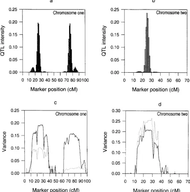
the MCMC samples. The posterior QTL intensities for can be expressed as

data I and II are presented in Figures 2 and 3,

respec-tively. The QTL intensity graphs are concentrated _f

a(⌬k)⫽

兺

104

m⫽1

兺

l(m)

q⫽1␴2aq1(␭ (m) q 苸⌬k)

兺

104

m⫽1

兺

l

(m)

q⫽11(␭(qm)苸⌬k)

around the true locations of the simulated QTL. Three peaks of the graph for data I appear in [24, 25] and

and [75, 76] on chromosome 1 and in [24, 25] on

chromo-some 2. The corresponding peaks for data II are in [25,

fd(⌬k)⫽

兺

104

m⫽1

兺

l(m)

q⫽1␴2dq1(␭ (m) q 苸⌬k)

兺

104

m⫽1

兺

l

(m)

q⫽11(␭(qm)苸⌬k)

, 26] and [75, 76] on chromosome 1 and in [25, 26] on

chromosome 2. These results not only support quite

strongly a model having three QTL but also indicate respectively, wherel(m)_{is the number of QTL in themth}

posterior sample,␭(m)

q is Note thatfa(⌬k) andfd(⌬k) are

that the QTL locations are estimated accurately for both

data sets. Finally, we noted that it took only a few thou- meaningful only when a sufficient number of samples are contained in ⌬k. The plots of fa(⌬k) andfd(⌬k) for

sand iterations for QTL locations to converge to their

stationary states, regardless of which initial position was data I are presented in Figure 2. The chromosome re-gions with sufficiently high posterior QTL intensity are chosen, indicating that the algorithm for updating QTL

locations is very efficient. given in Table 3. The posterior samples in which QTL

locations fell into these regions were used to estimate The overall mean and the residual variance were

esti-mated from all MCMC samples. The posterior distribu- the QTL variances. Figure 5 depicts the posterior

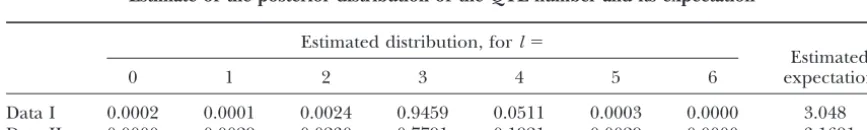
distri-TABLE 2

Estimate of the posterior distribution of the QTL number and its expectation

Estimated distribution, forl⫽

Estimated

0 1 2 3 4 5 6 expectation

Data I 0.0002 0.0001 0.0024 0.9459 0.0511 0.0003 0.0000 3.048

Figure 2.—Histograms of the posterior QTL intensity (a and b), and QTL allelic and dominance variance estimates (c and d) over two chromo-somes with bin length of 1 cM for the analysis of data I. In c and d, the solid and dotted curves represent allelic and dominance variances, respec-tively.

butions for the QTL variances from the analysis of data the distributions of allelic and dominance effects of QTL,i.e.,p(aj) andp(dj), are treated as priors or not.

I. We also calculated the means and the standard errors

of the posterior samples for the QTL variances (see If they are treated as prior distributions, the parameters involved in the prior distributions are assessed before Table 3). In most situations, it appears that the estimates

of QTL variances are close to the corresponding true the experiment, and there is no attempt to estimate

them. The model is then called the fixed model. On values with small standard errors. The posterior means

and the estimation errors of the QTL locations are also the other hand, ifp(aj) andp(dj) are not the ultimate

priors but the distribution of missing valuesaj and dj,

given in Table 3. It can be seen that the estimated QTL

locations are very close to the corresponding true values. we are then interested in the parameters in p(aj) and p(dj),e.g.,␴2aj, which in turn need to be assigned a prior.

We are essentially interested in making an inference DISCUSSION

for␴2

aj. In this case, the model is called a random model.

For the fixed model, the update steps for QTL variances There are many statistical methods and computer

programs available for QTL mapping. Most of them are in the proposed algorithm are no longer required.

Therefore, programming-wise, the difference between specialized in one or two particular types of designs,

e.g., BC, F2, or multiple nuclear families. Here, we intro- a random and a fixed model depends on the turning

on/off of a single statement. duce a unified methodology of QTL mapping for

arbi-trarily complicated mating designs, ranging from a sim- The ability to handle arbitrarily complicated

pedi-grees and the flexibility of switching between fixed and ple line cross to multiple independent sib-pairs. Although

we developed the method based on a random-model random models possessed by our Bayesian mapping

arise from the use of an “allelic approach” as opposed approach, it works equally well for a fixed model. The

difference between the random and the fixed models to the traditional “genotypic approach.” In this study,

Figure4.—Approximate posterior distributions of the

over-Figure3.—Histograms of the posterior QTL intensity over all mean (a) and residual variance (b) for data I. chromosomes 1 (a) and 2 (b) with bin length of 1 cM for the

analysis of data II.

with discrete effects, we can modify the update steps (c) and (d) in the proposed algorithm. Assume that rather than the genotypic values. We also sampled the

there arekalleles at a certain QTL with allelic effects “allelic inheritance” from parents to offspring rather

{ai}ki⫽1, dominance effects {dij}iⱖj, and frequencies {pi}ki⫽1

than sampling the “genotypic transition.” As a result,

in the base population, wherepi,ai, and dijare the

fre-there is no need to consider the number of alleles and

quency and effect of theith allele and the dominance the total number of genotypes per locus in the mapping

effect between alleles i andj, respectively. The priors population. Instead, consideration is needed only when

for ai anddij can be assigned as independent normal

we assess the prior distribution of the founder alleles.

with known mean and variance. The prior for {pi}ki⫽1can

This treatment has greatly simplified the algorithm and

take a symmetric Dirichlet. In this case, the parameters increased the robustness of the method.

of interest are {ai}ki⫽1, {dij}iⱖj, and {pi}ki⫽1. The frequencies

In QTL mapping experiments of plants, founders are

{pi}ki⫽1can be updated using a Gibbs sampler because its

not usually a random sample from a reference

popula-full conditional distribution also remains Dirichlet tion. They are often selected to be complementary for

(Gelman et al. 1995; Richardson and Green 1997). some traits of interest. As a consequence, the

fixed-To update allelic effects {ai}ki⫽1 and dominance effects

model approach can be used. Under a random model,

{dij}iⱖj, we first simulate a proposal for each parameter

however, the update steps for the additional parameters

by using a random walk, then update the alleles of each included in the priors p(aj) and p(dj) depend on the

founder by sampling from a multinomial distribution, form of their prior distributions. We have only

ex-and finally use the Metropolis-Hastings algorithm to plained the reversible jump MCMC algorithm under

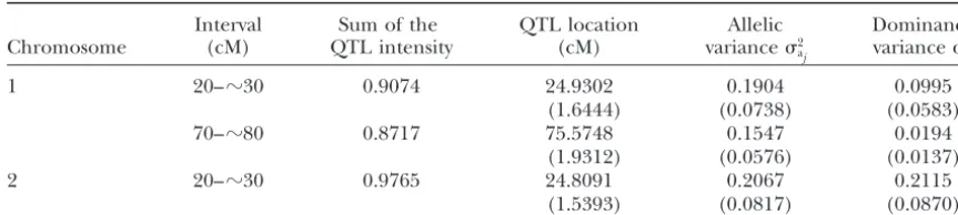
bial-TABLE 3

Highest posterior QTL intensity interval, Bayesian estimates of QTL locations, and allelic and dominance variances

Interval Sum of the QTL location Allelic Dominance

Chromosome (cM) QTL intensity (cM) variance␴2

a_j variance␴2a_j

1 20–ⵑ30 0.9074 24.9302 0.1904 0.0995

(1.6444) (0.0738) (0.0583)

70–ⵑ80 0.8717 75.5748 0.1547 0.0194

(1.9312) (0.0576) (0.0137)

2 20–ⵑ30 0.9765 24.8091 0.2067 0.2115

(1.5393) (0.0817) (0.0870)

Standard errors of the estimates are given in parentheses.

lelic QTL model have been proposed in Uimariand mixing of QTL locations in the simulation study. For

the normal QTL effects model, we found that the

Hoeschele(1997) andHeath(1997).

A problem may arise in real data analysis in which method used inStephens andFisch(1998) and

Sil-lanpa¨a¨ and Arjas (1998) resulted in QTL position the number of alleles of a putative QTL in the base

population is unknown, nor are the distributions of the stuck within the starting marker interval;i.e., the chain was essentially reducible. Furthermore, our algorithm effects of the QTL. In this situation, two strategies

should be considered: was much simpler than those of Heath (1997) and

Binket al.(2000). Second, the mixing of QTL number 1. We can use the fixed-model approach to solve the

was sensitive to the way in which the proposals for the random-model problem; that is, we first estimate the

new QTL were generated when one QTL was added to allelic and dominance effects of founders and then

the model and one QTL was removed from the model.

convert them into the QTL variances (Xu 1998).

The proposal distribution of allelic inheritance matrix This method is expected to be efficient in the case

Zp

l⫹1andZml⫹1was crucial for the reversible jump step to

where the number of founders is small.

perform well. It was found that QTL number mixed 2. In the case of many founders, one may use normal

poorly when p(Zp

l⫹1, Zml⫹1|␭l⫹1, GLl⫹1, GRl⫹1) was used to

distributions to approximate the prior distributions

generateZp

l⫹1andZml⫹1 in the normal-effects model ap-p(aj) andp(dj). In fact, drawing inferences about the

proach, although such proposal distributions of the ge-multiallelic QTL variance via the normal distribution

notypes of new QTL worked well in line crosses and the is a natural way to characterize genetic variation in

biallelic-effects model (Uimari andHoeschele 1997; the base population. In addition, normal distribution

Sillanpa¨a¨andArjas1998, 1999). Third, we found very of the allelic effects is usually a very robust

assump-little influence of the starting values of unknowns on tion. This has been verified in the context of ML

the mixing of the number of QTL. For example, starting

mapping by Xu and Atchley (1995) who found

withl0⫽6,lquickly dropped to 3 after several hundred

that, for data simulated under a biallelic model, the

iterations and subsequently behaved the same as that analysis based on normal distribution provided very

started withl0⫽3. We also found that the convergence

accurate estimates of QTL variances.

speed of different parameters was quite different. As expected, the dominance variance converged most Further investigation is needed to investigate the

ro-slowly due to too many dominance effects in the simu-bustness of normal distribution or other distributions

lated data. Finally, the implement of the algorithm was in the framework of Bayesian analysis.

computationally demanding due to the intricacy of our The proposed reversible jump MCMC algorithm

per-MCMC sampler. The analysis of data I with a chain of formed well for the simulated data. The following points

5⫻105_{cycles took}ⵑ_{3 days on a SUN SPARC 5}

worksta-are noteworthy. First, the update step of QTL locations is

tion. The most time-consuming parts of our program different from existing algorithms in Bayesian mapping

were the updates of complete marker genotypes, QTL (e.g., Satagopan et al. 1996; Heath 1997; Stephens

allelic inheritance, and dominance design matrices. The andFisch1998;Sillanpa¨a¨andArjas1998, 1999;Bink

computational speed can be improved substantially with

et al. 2000). We updated QTL location, allelic

inheri-more efficient programming skills. tance, and dominance design matrices simultaneously.

The assessment of the convergence and autocorrela-The acceptance probability depended on the proposed

tion of the MCMC with the use of the reversible jump location, the genotypes of flanking loci of the proposed

sampler remains a significant problem because the di-location (markers or QTL), and the phenotypic value

mension keeps changing from one cycle to another. of the progeny as well as other parameter values in

Figure5.—Approximate poste-rior distributions of the QTL al-lelic and dominance variances for data I. (a and b) Allelic and domi-nance variances determined from

interval 20–ⵑ30 cM of

chromo-some one, respectively; (c and d) allelic and dominance variances

determined from interval 70–ⵑ80

cM of chromosome 1, respectively; (e and f ) allelic and dominance variances determined from

inter-val 20–ⵑ30 cM of chromosome 2,

respectively.

also change. The parameters in one cycle of the iteration chain, and the interval length of subsampling to reduce the serial correlation. We used the plots of the changes may be different from those in the next cycle of

itera-tion. Therefore, the convergence criteria developed for in the number of QTL against the number of iterations to determine an approximate burn-in period (plots not the MCMC with fixed dimension are hardly applicable

to the reversible jump MCMC (e.g.,Brooks1997). In shown). The length of subsampling intervals was chosen to eliminate obvious changing trends for all parameters. our simulation study, therefore, we empirically

line-quantitative trait loci in outbred populations with incomplete

cross designs (e.g.,Sillanpa¨a¨andArjas1998), the

ac-marker data. Genetics151:409–420.

ceptance rates for adding a new QTL to the model and _{Bink, M. C. A. M., L. L. G. JanssandR. L. Quaas,2000 Markov chain}

Monte Carlo for mapping a quantitative trait locus in outbred

deleting a QTL from the model in our simulation were

populations. Genet. Res.75:231–241.

relatively low. This result is expected because too many

Brooks, S. P.,1997 Discussion to Richardson and Green (1997). J.

new values need to be generated for a birth step in the _{R. Stat. Soc. Ser. B59:774–775.}

Cantet, R. J. G.,andC. Smith,1991 Reduced animal model for

complicated mating design. The acceptance proportion

marker assisted selection using best linear unbiased prediction.

for updating QTL locations was rather high (ⵑ75%).

Genet. Sel. Evol.23:221–233.

We used the method of Bink and Van Arendonk _{Fernando, R. L.,andM. Grossman,1989 Marker-assisted selection}

using best linear unbiased prediction. Genet. Sel. Evol.21:467–

(1999) to update marker genotypes in the simulation

477.

study. This method is established on a marker-by-marker

Gelman, A. J. B., H. S. Carlin, H. S. SternandD. B. Rubin,1995

and individual-by-individual basis. In general, this kind _{Bayesian Data Analysis.Chapman & Hall, London.}

Geman, S.,andD. Geman,1984 Stochastic relaxation, Gibbs

distribu-of single-site update does not always lead to an

irreduc-tions, and the Bayesian restoration of images. IEEE Trans. Pattern

ible sampler because of the strong dependency of close

Anal. Machine Intell.6:721–741.

relatives and strong dependency of adjacent loci. In our _{Green, P. J.,1995 Reversible jump Markov chain Monte Carlo}

com-putation and Bayesian model determination. Biometrika82:711–

simulation study, we did not find insufficient mixing in

732.

marker genotype sampling, because the marker loci

Hastings, W. K.,1970 Monte Carlo sampling methods using Markov

were not tightly linked. However, a block sampling,e.g., _{chains and their applications. Biometrika57:97–109.}

Heath, S. C.,1997 Markov chain Monte Carlo segregation and

the genotypes at a given locus being updated

simultane-linkage analysis for oligogenic models. Am. J. Hum. Genet.61: ously for all individuals or sampling several loci jointly,

748–760.

is expected to be preferred over a single-site sampling _{Hoeschele, I., P. Uimari, F. E. Grignola, Q. ZhangandK. M. Gage,}

1997 Advances in statistical methods to map quantitative trait

in complex pedigrees and tightly lined loci. Such a

sam-loci in outbred populations. Genetics147:1445–1457.

pling strategy will be incorporated into the proposed

Jansen, R. C.,1993 Interval mapping of multiple quantitative trait

algorithm. The marker genotype sampler used in this loci. Genetics135:205–211.

Kao, C. H., Z. B. ZengandR. D. Teasdale,1999 Multiple interval

study is suitable only in the case where there is no

miss-mapping for quantitative trait loci. Genetics152:1203–1216.

ing marker nonfinal offspring. When there are missing _{Lander, E. S.,andD. Botstein,1989 Mapping Mendelian factors} markers in nonfinal offspring, more sophisticated sam- underlying quantitative traits using RFLP linkage maps. Genetics

121:185–199.

plers,e.g., the descent graph sampler (SobelandLange

Lynch, M.,andB. Walsh,1998 Genetics and Analysis of Quantitative 1996), are required to update the marker complete _{Traits.Sinauer Associates, Sunderland, MA.}

genotypes. The descent graph sampler can be used to Metropolis, N., A. W. Rosenbluth, M. N. Rosenbluth, A. H. TellerandE. Teller,1953 Equation of state calculations by

sample the gene flow patterns in arbitrarily complicated

fast computing machines. J. Chem. Phys.21:1087–1091.

pedigrees. This powerful computational algorithm can _{Muranty, H.,1996 Power of tests for quantitative trait loci detection}

be incorporated into our model. using full-sib families in different schemes. Heredity76:156–165.

Richardson, S., and P. J. Green, 1997 On Bayesian analysis of

Following the convention in human pedigree analysis,

mixtures with an unknown number of components. J. R. Stat.

we have assumed that all founders are included in the _{Soc. Ser. B59:731–792.}

model. In open-pollinated trees, however, seeds col- Satagopan, R. J.,andB. S. Yandell,1996 Estimating the number of quantitative trait loci via Bayesian model determination. Special

lected from one tree (mother) are usually pollinated

Contributed Paper Session on Genetic Analysis of Quantitative

from multiple unknown trees (fathers). Because the _{Traits and Complex Diseases. Biometric Section, Statistical} Meet-fathers (founders) are not identified, their contribution ing, Chicago, IL.

Satagopan, J. M., B. S. Yandell, M. A. NewtonandT. G. Osborn,

to the progeny is difficult to evaluate. Our model, in

1996 A Bayesian approach to detect quantitative trait loci using

theory, can include these founders in the pedigree but _{Markov chain Monte Carlo. Genetics144:805–816.}

Schork, N. J.,1993 Extended multipoint identity-by-descent analysis

treat their marker genotypes as missing. A method that

of human quantitative traits: efficiency, power, and modeling

excludes the missing founders while still analyzing the

considerations. Am. J. Hum. Genet.53:1306–1319.

data properly is under development. _{Sillanpa¨a¨, M. J.,andE. Arjas,1998 Bayesian mapping of multiple}

quantitative trait loci from incomplete inbred line cross data. We thank Claus Vogl and Lori Weingartner for helpful comments

Genetics148:1373–1388. on the manuscript. This research was supported by the National

Insti-Sillanpa¨a¨, M. J.,andE. Arjas,1999 Bayesian mapping of multiple tutes of Health grant GM55321 and the U.S. Department of Agricul- _{quantitative trait loci from incomplete outbred offspring data.} ture National Research Initiative Competitive Grants Program 97- _{Genetics151:1605–1619.}

35205-5075 to S.X. Slate, J., J. M. Pembertonand P. M. Visscher,1999 Power to

detect QTL in a free-living polygynous population. Heredity83:

327–336.

Sobel, E.,andK. Lange,1996 Descent graphs in pedigree analysis: applications to haplotyping, location scores, and marker-sharing

LITERATURE CITED

statistics. Am. J. Hum. Genet.58:1323–1337.

Almasy, L.,andJ. Blangero,1998 Multipoint quantitative-trait link- Stephens, D. A.,andR. D. Fisch,1998 Bayesian analysis of quantita-age analysis in general pedigree. Am. J. Hum. Genet.62:1198– tive trait locus data using reversible jump Markov Chain Monte

1211. Carlo. Biometrics54:1334–1347.

Amos, C. I., 1994 Robust variance-components approach for as- Uimari, P.,andI. Hoeschele,1997 Mapping linked quantitative sessing genetic linkage in pedigrees. Am. J. Hum. Genet. 54: trait loci using Bayesian analysis and Markov chain Monte Carlo

535–543. algorithms. Genetics146:735–743.

Weller, J. I., Y. KashiandM. Soller,1990 Power of daughter and

granddaughter designs for determining linkage between marker

loci and quantitative trait loci in dairy cattle. J. Dairy Sci. 73: _Var(aj k)⫽ ␴2aj

冢

1 fk

fk 1

冣

, (Var(aj

k))⫺1⫽

1

␴2 aj(1⫺f

2 k)

冢

1 ⫺fk

⫺fk 1

冣

2525–2537.

Wijsman, E. M.,andC. I. Amos,1997 Genetic analysis of simulated

oligogenic traits in nuclear and extended pedigrees: summary and

of GAW10 contributions. Genet. Epidemiol.14:719–735.

Xu, S.,1998 Mapping quantitative trait loci using multiple families of line crosses. Genetics148:517–524.

Var(dj kk)⫽ ␴2d_j

冢

1 fk fk

fk 1 fk

fk fk 1

冣

,

Xu, S.,andW. R. Atchley,1995 A random model approach to interval mapping of quantitative trait loci. Genetics141:1189– 1197.

Yi, N.,andS. Xu,2000 Bayesian mapping of quantitative trait loci for complex binary traits. Genetics155:1391–1403.

(Var(dj kk))⫺1⫽

1 ␴2

d_j(1⫹fk)(1⫹2fk)

冢

1⫹fk ⫺fk ⫺fk ⫺fk 1⫹fk ⫺fk

⫺fk ⫺fk 1⫹fk

冣

.

Zeng, Z. B.,1993 Theoretical basis of separation of multiple linked gene effects on mapping quantitative trait loci. Proc. Natl. Acad. Sci. USA90:10972–10976.

If fk ⫽ 1 and fk⬘ ⬆ 1, then djkk⬘(1) ⫽ djkk⬘(2) and djkk⬘(3) ⫽

Communicating editor:Y.-X. Fu dj

kk⬘(4). Therefore,djkk⬘is equivalent to the 2⫻1 normal

random vector (dj

kk⬘(1),djkk⬘(3))T, with covariance

APPENDIX _␴2

dj

冢

1 fk⬘ fk⬘ 1

冣

.

The prior distributions for allelic and dominance ef-fects of the founders:Denoteaj

kas a 2 ⫻ 1 vector for Similarly, iffk⬘⫽1 and fk⬆1,djkk⬘ is equivalent to 2⫻

the allelic effects of the kth founder at the jth QTL, 1 normal random vector (dj

kk⬘(1),djkk⬘(2))T, with covariance

anddj

kk⬘ as a vector of interaction effects (dominance

effects) between thekth and thek⬘th founder alleles at _␴2

dj

冢

1 fk fk 1

冣

. thejth QTL. The dimension ofdj

kk⬘is 3 or 4, depending

on whetherkequalsk⬘. Explicitly,aj

k⫽(ajk(1),akj(2))T,djkk⫽ _{Finally, for the case wheref}

k⬆1 andfk⬘⬆1, we can get

(dj

kk(1),djkk(2),djkk(3))T, anddjkk⬘⫽(dkkj⬘(1),djkk⬘(2),djkk⬘(3),djkk⬘(4))T

(k⬆k⬘). The dimension ofdj

kkis 3 because each founder

carries two alleles and potentially contributes 3 possible interactions in the descendants. The dimension ofdj

kk⬘ Var(djkk⬘)⫽ ␴2dj

冢

1 fk fk⬘ fkfk⬘ fk 1 fkfk⬘ fk⬘ fk⬘ fkfk⬘ 1 fk fkfk⬘ fk⬘ fk 1

冣

, is 4 because 2 founders carry a total of 4 alleles and

potentially contribute 2⫻ 2⫽ 4 possible interactions. The priors foraj

kanddjkk⬘are assumed to be indepen- _and

dent normals:

aj

kⵑN(0, Var(ajk)), dkkj ⬘ⵑN(0, Var(djkk⬘)).

(Var(dj

kk⬘))⫽_␴2 1

dj(1⫺f

2

k)(1⫺f2k⬘)

冢

1 ⫺fk ⫺fk⬘ fkfk⬘ ⫺fk 1 fkfk⬘ ⫺fk⬘ ⫺fk⬘ fkfk⬘ 1 ⫺fk

fkfk⬘ ⫺fk⬘ ⫺fk 1

冣

.

If the inbreeding coefficient, fk, for the kth founder

equals 1, the two elements of aj

kare identical, and so

are the three elements ofdj

kk. Therefore,ajkanddjkkeach

Under the assumption that the founders are indepen-turns into a scalar, aj

k(1) and djkk(1). Similarly, if both fk

dent from each other, the priorsp(aj) andp(dj) can be

and fk⬘ are unity, djkk⬘(1) ⫽ djkk⬘(2) ⫽ djkk⬘(3) ⫽ djkk⬘(4). Note

expressed as the following forms, respectively: that ␴2

aj and ␴ 2

dj are set at prefixed constants under a

fixed model. Otherwise, they are treated as unknown

p(aj)⫽

兿

m

k⫽1 p(aj

k) and p(dj)⫽

兿

m

k⫽1

兿

m

k⬘⫽k p(dj

kk⬘).