Strong approximations for resample quantile processes and
application to ROC methodology
Jiezhun Gu 1, Subhashis Ghosal2 3
Abstract
The receiver operating characteristic (ROC) curve is defined as true positive rate versus
false positive rate obtained by varying a decision threshold criterion. It has been widely used
in medical science for its ability to measure the accuracy of diagnostic or prognostic tests.
Mathematically speaking, ROC curve is a composition of survival function of one population
to the quantile function of another population. In this paper, we study strong approximation
for the quantile processes of bootstrap and the Bayesian bootstrap resampling distributions,
and use this result to study strong approximations for the empirical ROC estimator, the
corresponding bootstrap, and the Bayesian versions in terms of two independent Kiefer
processes. The results imply asymptotically accurate coverage probabilities for bootstrap
and the Bayesian bootstrap confidence bands, and accurate frequentist coverage probabilities
of bootstrap and the Bayesian bootstrap confidence intervals for the area under the curve
functional of the ROC.
Key words: Bayesian bootstrap; Bootstrap; Empirical process; Kiefer process; ROC
curve; Strong approximations.
1Department of Statistics, North Carolina State University, Raleigh, NC 27695. Email:
2Department of Statistics, North Carolina State University, Raleigh, NC 27695. Email:
1
Introduction
Originally introduced in the context of electronic signal detection (Green and Swets, 1966),
the receiver operating characteristic (ROC) curve, which is a plot of the true positive rate
versus the false positive rate, has become a popular method for measuring the accuracy of
diagnostic tests since the 1970s (Metz, 1978). The true positive rate and the false positive
rate can be obtained by varying the threshold criterion. The main attractions of ROC curve
may be described by the following properties: (1) it can display the trade-off between the
true positive rate and false positive rate by varying the decision threshold values in a unit
graph; (2) it can be compared with ROC curves of other diagnostic tests, even with different
measurements of the diagnostic variables. The area under the curve (AUC) functional of
ROC can be interpreted as the probability that the diagnostic value of a randomly chosen
patient with the positive condition (usually referring to disease) is greater than the
diag-nostic value of a randomly chosen patient without the positive condition. A nonparametric
estimator of ROC may be obtained by substituting into the empirical distributions, and its
variability may be estimated by bootstrap (Pepe, 2003). More recently, Gu et al. (2006)
pro-posed a smoother estimator and related confidence bands by using the Bayesian bootstrap
(BB) method. In this paper, we develop strong approximations of bootstrap and BB quantile
process by a sequence of appropriate Gaussian processes (more specifically, Kiefer processes).
Combining these results with some earlier results from strong approximation theory in an
appropriate way, we shall develop strong approximations for the empirical, bootstrap and
BB version of the ROC process, its AUC and other functionals. In particular, these results
imply a Gaussian weak limit for the processes and asymptotically valid coverage probabilities
for the resulting confidence bands and intervals.
• Koml´os, Major and Tusn´ady (1975) showed that the uniform empirical process can be strongly approximated by a sequence of Brownian bridges obtained from a single
Kiefer process;
• Cs¨org˝o and R´ev´esz (1978) proved that under suitable conditions quantile process can be strongly approximated by a Kiefer process;
• Lo (1987) studied the strong approximation theory for the cumulative distribution function (c.d.f.) of bootstrap and BB processes.
In this paper, we will first obtain strong approximations for quantile processes of
resam-pling processes based on the bootstrap and the BB. The ROC function isR(t) = ¯G( ¯F−1(t)),
where ¯F(x) = 1−F(x) and ¯G(y) = 1−G(y) are the survival functions of independent vari-ables X ∼ F and Y ∼ G. As a consequence, we will obtain the strong approximations for the empirical estimate of R(t) and the corresponding bootstrap, and the Bayesian versions of R(t). Interestingly, it will be seen that the forms of these Gaussian approximations are identical, and therefore the distribution of the ROC function, conditioned on the samples,
is identical to the Gaussian approximation of the empirical ROC estimate. This means that
frequentist variability of the empirical estimate of ROC can be asymptotically accurately
estimated by resampled variability of bootstrap and BB procedures, given that the
sam-ples and the “posterior”mean (i.e, mean of ROC under BB distribution) are asymptotically
equivalent to that of the empirical estimate up to the first order (O(N−1/2)), where N is
the total sample size. Also, the result implies that for functionals like AUC, the empirical
estimator is asymptotically normal and asymptotically equivalent to the BB estimator, and
2
Notation
2.1
Preliminary notation
Before introducing the notations for empirical and quantile processes, we will define some
commonly used notation:
1. Define the domain of X as [a, b]: a = sup{x : F(x) = 0}, b = inf{x : F(x) = 1}; For a given 0 < y < 1, k = ⌈ny⌉, where ⌈·⌉ is the ceiling function, that is, the smallest integer greater than or equal to x. U(0,1) denotes the uniform distribution on [0,1]; Abbreviate almost sure convergence by a.s.; Define inverse of a general c.d.f. as follows: F−1(t) = inf{x : F(x) ≥ t}, t ∈ [0,1]; X
1, ..., Xn ∼ i.i.d. F, equivalently,
Xj = F−1(Uj), where U1, . . . , Un ∼ i.i.d. U(0,1). Xj:n denote the jth largest order statistic based on {X1, . . . , Xn}, j = 0,1, . . . , n+ 1, where X0:n = a, Xn+1:n =b. We define Vj:n,Uj:n in the same way in this paper.
2. Condition A(Cs¨org˝o and R´ev´esz, 1978): LetX1, . . .be i.i.d. random variables with a
continuous distribution functionF which is twice differentiable on (a, b), whereF′ =f
6
= 0 on (a, b). For some γ >0, supa<x<bF(x)(1−F(x))
f′
(x)
f2(x)
≤
γ.
3. Condition BLet F and G satisfy Condition A and the following conditions:
sup a<x<b
F(x)(1−F(x))
g′
(x)
f2(x)
, sup a<x<b
F(x)(1−F(x))
g(x)
f(x)
are bounded.
For example, if F = Normal(0,1), G = Normal(1,1) , then Condition A and B hold since limx→+∞
R∞
x xe−
(t2−x2)/2
dt = 2.
α−1
m =o(m1/4), αm∗ =αm + 2m−1/2(log logm)1/2, α#m =αm+ (m−1)−1/2(log log(m− 1))1/2. The symbol is used at the end of the proof.
2.2
Empirical and quantile functions:
ForX1, ..., Xn ∼ i.i.d. F,
empirical function: Fn(x) = j/n, if Xj:n ≤x < Xj+1:n, j = 0,1, . . . , n. (1)
empirical process: Jn(x) = √n(Fn(x)−F(x)) (2)
quantile function: F−n1(y) = Xk:n=F−1(Uk:n), wherek =⌈ny⌉ (3)
quantile process: Qn(y) =√n(Fn−1(y)−F−1(y)) (4)
In particular, we will study bootstrap and BB resampling quantile processes.
2.2.1 Resampling distribution under bootstrap
X1, . . . , Xn ∼ i.i.d. F, bootstrap resample is given by {F−n1(Vj:n), j = 1, . . . , n;V1, . . . , Vn ∼ i.i.d. U(0,1) independent of Xi’s }. The empirical and quantile functions of bootstrap re-sampling distribution are denoted asF∗n(x) andF∗−n 1(y), respectively, based on the bootstrap resamples. Bootstrap empirical and quantile processes are defined as
J∗n(x) =√n(Fn∗(x)−Fn(x)) (5)
Qn∗(y) = √n(Fn∗−1(y)−F−n1(y)) =√n(F−n1(Vk:n)−F−n1(y)) = √
n(F−1(Uk∗
:n)−F−1(Uk:n)),
(6)
where k=⌈ny⌉, k∗ =⌈nV
2.2.2 Resampling distribution under BB
ForX1, ..., Xn ∼ i.i.d. F, BB distribution (c.d.f.) is defined as follows:
F#n(x) = X
1≤j≤n
∆j:n1(Xj:n≤x) x∈R,
whereV1, . . . , Vn−1∼i.i.d. U(0,1), independent ofXi’s, ∆j:n =Vj:n−1−Vj−1:n−1,j = 1, . . . , n.
The BB quantile function is defined as follows:
F#n−1(y) =
Xk:n, Vk−1:n−1 < y ≤Vk:n−1, k = 1,2, . . . , n,
X0:n, y= 0.
BB empirical and quantile processes are defined as follows:
J#n(x) = √n(Fn#(x)−Fn(x)), (7)
Q#n(y) = √n(Fn#−1(y)−F−n1(y)). (8)
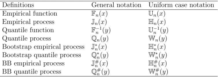
Table 1: Notation for empirical and quantile processes
Definitions General notation Uniform case notation Empirical function Fn(x) Un(x)
Empirical process Jn(x) Hn(x) Quantile function F−n1(y) U−n1(y) Quantile process Qn(y) Wn(y) Bootstrap empirical process J∗n(x) H∗n(x) Bootstrap quantile process Q∗n(y) W∗n(y) BB empirical process J#
3
Strong approximations for bootstrap and BB
quan-tile processes
Theorem 3.1(Strong approximation for bootstrap quantile process ) LetX1, X2, . . .∼i.i.d.
F satisfying Condition A. Then the quantile process of bootstrap Q∗n(y) can be strongly approximated by a Kiefer process K, in the sense that
sup δ∗
n≤y≤1−δ ∗ n
|f(F−1(y))Q∗n(y)−n−1/2K(y, n)|=a.s.O(ln). (9)
To prove this theorem, we need the following lemma whose proof is given in Section 5.
Lemma 3.1LetX1, . . . , Xn ∼i.i.d. F satisfying Condition A, and letV1, . . . , Vn ∼i.i.d.
U(0,1), independent of X1, ..., Xn. Then for the quantile process Qn(y) ofXi’s, there exists
a Kiefer process K such that
sup δ∗
n≤y≤1−δ ∗ n
|f(F−1(y))Qn(Vk:n)−n−1/2K(y, n)|=a.s.O(ln), (10)
where k=⌈ny⌉.
Proof of Theorem 3.1 :
When δ∗
n≤ y≤1−δn∗, [δn∗,1−δn∗]⊂[δn,1−δn]. Let k =⌈ny⌉ and k∗ =⌈nVk:n⌉. Then
Q∗n(y) can be split into summation of three parts as Qn(Vk:n) + ˜Qn(y)−Qn(y), where Qn(y)
and ˜Qn(y) are independent quantile processes forXi’s and ˜Xi’s respectively, Xi =F−1(Ui), ˜
Xi = F−1(Vi), Ui ∼ i.i.d. U(0,1), Vi ∼ i.i.d. U(0,1), and Ui’s and Vi’s are independent,
i= 1, . . . , n. By Theorem B of Appendix and Lemma 3.1, Theorem 3.1 is immediate. Theorem 3.2 (Strong approximation for the BB quantile process) LetX1, ..., Xn∼i.i.d.
by a Kiefer processK, in the sense that
sup δ#n≤y≤1−δ
#
n
|f(F−1(y))Q#n(y)−n−1/2K(y, n)|=a.s. O(ln). (11)
The proof requires the following lemma whose proof is deferred to Section 5.
Lemma 3.2 Let X1, . . . , Xn ∼ i.i.d. F satisfying Condition A, V1, . . . , Vn−1 ∼ i.i.d.
U(0,1),F−n1(y), ˜Un−1(x) andF#n−1(y) denote the quantile function ofX’s , empirical function of V’s and quantile function of the Bayesian bootstrap respectively. Then
sup
0<y<1
√
n|F#n−1(y)−F−n1( ˜Un−1(y))|=a.s O(n−1/2logn), (12)
In addition, there exists a Kiefer process K, such that
sup δ#n≤y≤1−δ
#
n
|√nf(F−1(y))(Fn−1( ˜Un−1(y))−Fn−1(y))−n−1/2K(y, n)|=a.s. O(ln). (13)
Proof of Theorem 3.2 :
We may represent Xi =F−1(Ui), whereUi’s∼ i.i.d. U(0,1), i= 1, . . . , n,V1, . . . , Vn−1 ∼
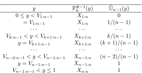
i.i.d. U(0,1), independent of X’s. Then we have (cf. See Table 2 for Values of F#−1
n (y) and ˜
Un−1(y))
F#n−1(y) =
F−n1(1+(n−1)˜Un−1(y)
n ), Vk:n−1 < y < Vk+1:n−1, k= 0, . . . , n−1,
F−n1((n−1)˜Un−1(y)
n ), y=Vk:n−1, k = 1, . . . , n−1.
Also, the BB quantile process Q#n(y) can be split as √n(F#n−1(y)− F−n1( ˜Un−1(y))) +
√
n(F−1
Table 2: Values of F#n−1(y) and ˜Un−1(y)
y F#−1
n (y) U˜n
−1(y)
0≤y < V1:n−1 X1:n 0
=V1:n−1 X1:n 1/(n−1)
· · · ·
Vk:n−1< y < Vk+1:n−1 Xk+1:n k/(n−1)
y=Vk+1:n−1 Xk+1:n (k+ 1)/(n−1)
· · · ·
Vn
−2:n−1< y < Vn−1:n−1 Xn−1:n (n−2)/(n−1) y=Vn
−1:n−1 Xn−1:n 1 Vn
−1:n−1< y≤1 Xn:n 1
4
Functional limit theorems for ROC curves and their
AUCs
4.1
Functional limit theorems for ROC curves
Let X1, X2, ..., Xm ∼ i.i.d. F, and Y1, Y2, ..., Yn ∼ i.i.d. G, which are c.d.f.’s of populations of interest. For example, in medical contexts F may stand for the c.d.f. of a population without disease and G for the c.d.f. of a population with disease. Assume F and G satisfy Condition A and B.
The ROC curve is defined as {(P(X > t), P(Y > t)) : X ∼ F , Y ∼ G , t ∈ R}, or alternatively asR(t) = ¯G( ¯F−1(t)); its derivative is R′(t) = g( ¯F−1(t))/f( ¯F−1(t)).
Theorem 4.1 ( Functional limit theorem for empirical, bootstrap and BB’s ROC curve
estimators, denoted as Rm,n(t), R∗m,n(t), R#m,n(t) respectively. ) Let X1, . . . , Xm ∼ i.i.d. F,
N =m+n, m N →λ,
n
N →1−λ. Then
Rm,n(t) =R(t) +R′(t)
K1(t, m)
m +
K2(R(t), n)
n +O(α
−1
m τm), t∈(αm,1−αm), (14)
R∗m,n(t) =Rm,n(t) +R′(t)K1(t, m)
m +
K2(R(t), n)
n +O(α
−1
m τm), t∈(α∗m,1−α∗m), (15)
R#m,n(t) =Rm,n(t) +R′(t)K1(t, m)
m +
K2(R(t), n)
n +O(α
−1
m τm), t∈(α#m,1−α#m). (16)
in the sense ofa.s. conditionally on the observed samples, whereK1 andK2 are independent
generic Kiefer processes (not identical in each appearance).
Proof of Theorem 4.1 :
1. Proof of (14) of Theorem 4.1: By Theorem A and B of Appendix, whent∈(αm,1−
αm)⊂(δm,1−δm), the empirical ROC curve estimatorRm,n(t) can be approximated by the following:
Rm,n(t) = ¯Gn(¯F−m1(t)) = ¯G(¯F−m1(t)) + 1
nK2( ¯G(¯F
−1
m (t)), n) +O(γn) = ¯G( ¯F−1(t)) + 1
nK2( ¯G( ¯F
−1(t)), n) +I
1+I2+O(γn),
where
I1 = ¯G(¯F−m1(t))−G¯( ¯F−1(t)) = m−1R′(t)K1(t, m) +O(αm−1τm), (17)
I2 =n−1K2( ¯G(¯Fm−1(t)), n)−n−1K2( ¯G( ¯F−1(t)), n) = O((m/n)1/2α−m1/2τm) (18)
Proof of (17) : By Theorem B of Appendix, we have
I1 =g( ¯F−1(t))
m−1K
1(t, m)−O(τm)
f( ¯F−1(t)) −g
′( ¯F−1(ξ))
m−1K
1(t, m)−O(τm)
f( ¯F−1(t))
and ξ lies between t and U⌈mt⌉:m, which ensures f( ¯F−1(ξ))/f( ¯F−1(t)) ≤ 10γ. By Condition B, we get
|R′(t)O(τm)|=
t(1−t)g( ¯F
−1(t))
f( ¯F−1(t))
O(τm)
t(1−t)
≤
O(αm−1τm) (19)
ξ(1−ξ)g
′( ¯F−1(ξ))
f2( ¯F−1(ξ))
f2( ¯F−1(ξ))
f2( ¯F−1(t))ξ(1−ξ)
(m−1K1(t, m)−O(τm))2
≤O(α−m1m−1log logm) a.s. (20)
By combining (19) and (20), we finish the proof of (17).
Proof of (18) : By modulus of continuity for Brownian motion on bounded interval, we get
|I2 |=|
1
nK2( ¯G(¯F
−1
m (t)), n)− 1
nK2( ¯G( ¯F
−1(t)), n)
|
≤n−1/2 |I1 |1/2 (log(1/|I1 |))1/2
≤n−1/2 | R′(t)
m K1(t, m) +O(α
−1
m τm)|1/2 (logm)1/2
≤n−1/2 |O(αm−1m−1/2(log logm)1/2) +O(α−m1τm)|1/2 (logm)1/2
=O((m/n)1/2αm−1/2τm) a.s. (21)
The proof of (14) is now complete.
2. Proof of (15) of Theorem 4.1: The idea of the proof of (15) is similar to (14),
except for the following: (1) A major difference is that Theorem 3.1 in Section 3 is used
instead of Theorem B of Appendix; (2) We can expand I∗
12 in Taylor’s series instead
of I∗
1, where I1∗ = ¯Gn(¯F∗−m1(t))−G¯n(¯F−m1(t)) =I11∗ +I12∗ , I12∗ = ¯G(¯F∗−m 1(t))−G¯(¯F−m1(t)),
I∗
estimator is expanded around the empirical estimator, the Taylor’s series expansion is
evaluated at the empirical point ¯F∗−m1(t) instead of at the true point ¯F−1(t). Measuring
these difference enlarges the range of domain fromt∈(αm,1−αm) tot∈(α∗m,1−α∗m), which allows the limiting distribution of bootstrap estimator to be the same as the
empirical estimator’s.
3. Proof of (16) of Theorem 4.1: The proof of (16) follows the same lines as the proof of (15) with the following modifications: (1) Theorem 3.2 is applied instead of Theorem
3.1 in Section 3; (2) In order to use Taylor’s series expansion and the boundedness
result of the ratio of ff( ¯( ¯FF−−11((ξt)))), whereξ lies between t and ˜Um−1(t), we will do Taylor’s
series expansion on I122# instead of I12#. That is, the decomposition I12# =I121# +I122# is essential, whereI12# = ¯G(¯F#m−1(t))−G¯(¯F−m1(t)),I121# = ¯G(¯F#m−1(t))−G¯(¯F−m1( ˜Um−1(t))),
I122# = ¯G(¯F−1
m ( ˜Um−1(t)))− G¯(¯F−m1(t)); (3) Similarly, one consequence of measuring the remainder term is to shrink the range of domain from t ∈ (α∗
m,1−α∗m) to t ∈ (α#
m,1−α#m).
4.2
Implication of the functional limit theorems for ROC curves
From (14), let N =m+n and assume that m N →λ,
n
N →1−λ, then asL∞[0,1] valued random function,
√
N(Rm,n(t)−R(t)) √1
λR
′(t)B
1(t) +
1 √
1−λB2(R(t)), (22)
in the sense of general weak convergence ( Van der Vaart & Wellner, 1996), where B1 and
conditionally on samples,
√
N(R∗m,n(t)−Rm,n(t)) √1
λR
′(t)B
1(t) +
1 √
1−λB2(R(t)), (23)
√
N(R#m,n(t)−Rm,n(t)) √1
λR
′(t)B
1(t) +
1 √
1−λB2(R(t)). (24)
Remark: We suspect that a possibly shorter approach to the distribution of (22), (23), (24) may be based on Donsker theorem, conditional Donsker theorem for bootstrap and
Hadamard differentiability (see Section 3.9 of Van der Vaart & Wellner, 1996). However,
calculation of Hadamard derivative of (F, G) 7−→ G¯ ◦ F¯−1 seems very challenging. The
approach based on strong approximation lets us work with real valued random variables
and ordinary Taylor’s series expansion, derive a stronger representation, and treat the whole
domain t ∈ [0,1] in the limit. In contrast, the weak convergence approach must leave out some neighborhoods of 0 and 1. From practical point of view, inclusion of levels near 0 is
important.
Result 1 For any continuity set A ⊂ L∞[0,1] of the process on the right hand side of
(22), interpreting probabilities as outer probabilities, then
Pr∗{√N(R∗m,n(·)−Rm,n(·))∈A} −Pr{ √
N(Rm,n(·)−R(·))∈A} →0. (25)
where Pr∗ stands for bootstrap probability conditional on samples.
Result 2 [Equivalence of empirical and BB estimator of ROC ]Conditionally on
samples,
√
4.3
Functional limit theorems for AUC
It is not difficult to show the following corollaries.
Corollary 1 Let ψ :R→R be a bounded function with continuous second derivatives,
N =m+n and assume that mN →λ, Nn →1−λ. Then as N → ∞, for any q >0 being the continuity point of the limiting random variable supt∈(0,1){ψ′(R(t))[λ−1/2R′(t)B
1(t) + (1−
λ)−1/2B
2(R(t))]}, interpreting probabilities as outer probabilities,
|Pr∗{ sup t∈(α∗
m,1−α ∗ m)
√
N |ψ(R∗m,n(t))−ψ(Rm,n(t))|≤q}
−Pr{ sup t∈(α∗
m,1−α ∗ m)
√
N |ψ(Rm,n(t))−ψ(R(t))|≤q} |→0, (27)
|Pr#{ sup t∈(α#m,1−α
#
m)
√
N |ψ(R#m,n(t))−ψ(Rm,n(t))|≤q}
−Pr{ sup t∈(α#m,1−α
#
m)
√
N |ψ(Rm,n(t))−ψ(R(t))|≤q} |→0, (28)
where Pr# stands for BB probability conditional on samples.
Remark: Equivalently, a metric d (such as Levy’s metric) which can characterize weak convergence can be also used to quantify the nearness of the distributions.
Corollary 2 Let φ(·) : C[0,1] → R be a bounded linear functional, N = m+n and assume that m
N → λ, n
N → 1−λ. Then as N → ∞, conditionally on the samples, we have for all q
Pr∗{√N(φ(R∗m,n)−φ(Rm,n))≤q} −Pr{ √
N(φ(Rm,n)−φ(R))≤q} →0 a.s. (29)
Pr#{√N(φ(Rm,n# )−φ(Rm,n))≤q} −Pr{√N(φ(Rm,n)−φ(R))≤q} →0 a.s. (30)
we have
√
N( ˆAm,n(α, β)−A(α, β))→N(0, σ2(α, β)), (31)
where σ2(α, β) = λ−1Rβ
α
Rβ
α R′(t)R′(s)(s ∧ t − st)dtds + (1 − λ)−
1Rβ
α
Rβ
α(R(t) ∧ R(s) −
R(t)R(s))dtds, ˆAm,n(α, β) =
Rβ
α Rm,n(t)dt, A(α, β) =
Rβ
α R(t)dt.
Remark: It can be easily shown that Condition B ensures the integrals in the expression
for σ(α, β) as α→0 and β→1.
5
Proof of the Lemmas in the sense of
a.s.
5.1
Proof of the Lemma 3.1
For any y ∈[δ∗
n,1−δ∗n], let k =⌈ny⌉. By applying Theorem D, K and N of Appendix, we can get
sup δ∗
n≤y≤1−δ ∗ n
|(y−Vk:n)Qn(Vk:n)f′(F−1(τ))/f(F−1(τ)))|=a.s. O(ln), (32)
for any τ lies between y and Vk:n. By Condition A, we have
f(F−1(y)) =f(F−1(Vk:n)) + (y−Vk:n)f′(F−1(ξ))/f(F−1(ξ)), (33)
where ξ lies between y and Vk:n. Note that y ∈ [δ∗n,1−δn∗] ensures that Vk:n ∈ [δn,1−δn]
5.2
Proof of the Lemma 3.2
5.2.1 Proof of the statement (12) of Lemma 3.2
By Theorem M, we have
sup
0<y<1
√
n|F#n−1(y)−Fn−1( ˜Un−1(y))|
≤ sup
0<y<1
√ n
F−n1 1 + (n−1) ˜Un−1(y)
n
!
−F−n1( ˜Un−1(y))
+ sup
0<y<1
√ n
F−n1 (n−1) ˜Un−1(y)
n
!
−F−n1( ˜Un−1(y))
≤ sup
0≤k≤n
2√n |Xk+1:n−Xk:n |=a.s. O(n−1/2logn).
5.2.2 Proof of the statement (13) of Lemma 3.2
Because y ∈ [δ#
n,1−δn#] ⊂ [ǫn,1−ǫn], where ǫn = 0.236n−1log logn, let k = ⌈ny⌉, ξ lies between y and ˜Un−1(y). The following four steps are needed to finish the proof.
1. By the similar argument as the proof of (32), we have supδ#
n≤y≤1−δ
# n
( ˜Un−1(y) −
y)ff′((FF−−11((ξξ))))Qn( ˜Un−1(y))
=a.sO(ln).
2. By Theorem B of Appendix, | √nf(F−1(y))(F−1
n (y)−F−1(y))−n−1/2K(y, n) |=a.s.
O(ln).
3. supδ#
n≤y≤1−δ
#
n |
√
nf(F−1(y))[F−1( ˜U
n−1(y))−F−1(y)]−n−1/2K(y, n)|can be bounded
by
sup δn#≤y≤1−δ
#
n
|√n( ˜Un−1(y)−y)−n−1/2K(y, n)|
+ sup
( ˜U (y)−y)2f′(F−
1(ξ))f(F−1(y))
which is O(ln) a.s.. The reasons for (34) are as follows:
(a) By Theorem A of Appendix, we have sup0<y<1p n n−1
√
n−1( ˜Un−1(y)−y)− K√(y,nn−−11)
=a.s.
O(√nlogn−2(1n−1)). By Theorems G and H of Appendix, we have sup0<y<1|n√−n1K(y, n−
1)−n−1/2K(y, n)|=a.s. O(ln). Therefore, the first term of (34) can be majorized
by sup0<y<1
p n n−1|
√
n−1( ˜Un−1(y)−y)−√n1−1K(y, n−1)|+sup0<y<1|
√
n
n−1K(y, n−
1)−n−1/2K(y, n)|=a.s. O(ln).
(b) By Theorem J of Appendix, we have ( ˜Un−1(y)−y)2 ≤a.s 4(n−1)−1y(1−y) log log(n− 1). By following a similar argument to that of Theorem 3 (Cs¨org˝o and R´ev´esz,
1978), we get ff((FF−−11((yξ)))) ≤10γ. Also by Condition A, the second term of (34) can be
majorized by supδ#
n≤y≤1−δ
#
n[4(n−1)
−1log log(n−1)]y(1−y)
ξ(1−ξ)ξ(1−ξ)
f′
(F−1(ξ))
f2(F−1(ξ))
f(F−1(y))
f(F−1(ξ)) ≤a.s.
O(ln).
4. By Theorems G and I of Appendix, we have sup0<y<1 √1
n−1 |K( ˜Un−1(y), n)−K(y, n)|=a.s.
O(ln).
Notice that F−1
n ( ˜Un−1(y))−F−n1(y) can be split as
[F−n1( ˜Un−1(y))−F−1( ˜Un−1(y))]−[Fn−1(y)−F−1(y)] + [F−1( ˜Un−1(y))−F−1(y)] (35)
By combining parts (1)- (4) above and plugging (35) into F−n1( ˜Un−1(y))−F−n1(y), we finish the proof of (13).
6
Appendix
Kiefer process: {K(x, y) : 0≤x≤1,0≤y <∞} is determined by K(x, y) =W(x, y)−
Kiefer process’s covariance function: E[K(x1, y1)K(x2, y2)] = (x1∧x2−x1x2)(y1∧
y2), where ∧ stands for the minimum.
The following theorems were used:
Theorem A: (Strong approximation for arbitrary empirical process) [Corollary of strong
approximation for uniform empirical process: Koml´os, Major and Tusn´ady, 1975]: Let
X1, X2, . . . ∼ i.i.d. F, whereF is any arbitrary continuous distribution function and Gn(x)
be the empirical process. Then there exists a Kiefer process{K(y, t); 0≤y ≤1, t ≥0}, such that
sup x
Jn(x)−n−1/2K(F(x), n)
=a.s. O(n−1/2log2n).
Theorem B: (Strong approximation for arbitrary quantile process) [Cs¨org˝o and R´ev´esz, 1978, Theorem 6]: Let X1, X2, . . . ∼ i.i.d. F, satisfying Condition A. Then the quantile
process Qn(x) of X can be approximated by a Kiefer process {K(y, t); 0≤y ≤1, t≥0}
sup δn≤y≤1−δn
|f(F−1(y))Qn(y)−n−1/2K(y, n)|=a.s.O(ln).
Theorem C: (Strong approximations for empirical processes of bootstrap and the
Bayesian Bootstrap) [Lo, 1987, Lemma 6.3]: There exists a Kiefer process {K(s, t); 0 ≤s≤
1, t≥0}independent of X such that
sup x |
J∗n(x)−n−1/2K(Fn(x), n)|=a.s.O(ln),
sup x |
J#n(x)−n−1/2K(Fn(x), n)|=a.s.O(ln).
Condition A. Then
lim sup n→∞
√
n
log lognδn≤supy≤1−δn
|f(F−1(y))Qn(y)−Wn(y)|≤40γ10γ a.s.
Theorem E: [Cs¨org˝o and R´ev´esz, 1981, Lemma 4.5.1]: Let U1, U2, . . . be i.i.d. U(0,1)
random variables, and let Kiefer process {K(y, t); 0 ≤ y ≤ 1,0 ≤ t} defined on the same probability space. Then
sup
1≤k≤n
n−1/2 |K(Uk:n, n)−K(k/n, n)|=a.s.O(ln).
Theorem F: [Cs¨org˝o and R´ev´esz, 1981,Theorem 1.15.2]: Lethnbe a sequence of positive numbers for which limn→∞ logh−n1
log logn =∞, γn= (2nhnlogh−
1
n )−1/2. Then
lim
n→∞0≤tsup≤1−hn
γn|K(t+hn, n)−K(t, n)|=a.s 1,
lim
n→∞0≤tsup≤1−hn
sup
0≤s≤hn
γn|K(t+s, n)−K(t, n)|=a.s 1.
Theorem G: Let K(s, n) be a Kiefer process,
sup
0<s<1
1 √
n−1
K(s, n−1)−K(s, n)
=a.s.O(ln).
Remark: Because Bn(s) = K(s, n)−K(s, n−1) is a series of independent Brownian bridges, this result follows immediately from the result of Lo (1987).
Theorem H: [Law of Iterated Logarithm (LIL)]: Let K(y, n) be Kiefer process,
lim sup n→∞
sup
0≤y≤1
|K(y, n)| (2nlog logn)12
=a.s. 1
Theorem I: [Special case of Lemma 6.2 (Lo, 1987) whenF =U(0,1)]: LetU1,· · · , Um∼ i.i.d. U(0,1), Um(s) is the empirical function of Ui’s. For any Kiefer process K independent of U1,· · · , Um,
sup
0<s<1
1 √
m |K(Um(s), m)−K(s, m)|=a.s.O(lm).
Theorem J: [Cs¨org˝o and R´ev´esz, 1978, Theorem D] : LetHn(x) be the uniform empirical process, ǫn = 0.236n−1log logn, then
lim sup
n→∞ǫn≤supx≤1−ǫn
(x(1−x) log logn)−1/2 |Hn(x)|=a.s. 2.
Theorem K: [Cs¨org˝o and R´ev´esz, 1978, Theorem 2]: LetWn(y) be the uniform quantile process, then
lim sup
n→∞δn≤supy≤1−δn
(y(1−y) log logn)−1/2 |Wn(y)|=a.s. 4.
Theorem L: [Cs¨org˝o and R´ev´esz, 1978, Lemma 1]: Under Condition A,
f(F−1(y 1))
f(F−1(y 2)) ≤
y1∨y2
y1∧y2 ·
1−y1∧y2
1−y1∨y2
γ
for any pair y1, y2 ∈(0,1).
Theorem M: [Slud, 1978]: Let U1, . . . , Un ∼ i.i.d. U(0,1) and define maximal uniform space Mn as Mn= max0≤k≤nUk+1:n−Uk:n. Then
nMn/logn →a.s1.
Theorem N: Important inequalities [Proof follows Cs¨org˝o and R´ev´esz, 1978, Theorem
For any y∈[δ∗
n,1−δ∗n]⊂[δn,1−δn], let k=⌈ny⌉,ξ lies between y and Vk:n. Then
y(1−y)
ξ(1−ξ) ≤5 (37)
ξ Vk:n ≤
5, 1−ξ
1−Vk:n ≤
5 (38)
sup δ∗
n≤y≤1−δ ∗ n
f(F−1(ξ))/f(F−1(Vk:n))≤10γ (39)
Remark: When y ∈ [δ#
n,1−δ#n], ξ lies between y and ˜Un−1(y). By Theorem J of
Ap-pendix, the inequalities (37), (38) and (39) hold fory, ξ and ˜Un−1(y) by the same arguments,
yielding
sup δn#≤y≤1−δ
#
n
y(1−y)
ξ(1−ξ) ≤5, (40)
sup δn#≤y≤1−δ
#
n
ξ
˜
Un−1(y) ≤5, δ# sup
n≤y≤1−δ
#
n
1−ξ
1−U˜n−1(y) ≤5, (41)
sup δn#≤y≤1−δ
#
n
f(F−1(ξ))/f(F−1( ˜Un−1(y)))≤10γ. (42)
7
References
1. Cs¨org˝o, M. and R´ev´esz, P. (1978). Strong approximations of the quantile process. The
Annals of Statistics 6, 882–894.
2. Cs¨org˝o, M. and R´ev´esz, P. (1981). Strong Approximations in Probability and Statistics.
Academic press, New York.
3. Green, D. M. and Swets, J. A. (1966). Signal Detection Theory and Psychophysics.
Institute of Statistics Mimeo Series 2592, NCSU.
5. Koml´os, J. , Major, P. and Tusn´ady, G. (1975). An approximation of partial sums of
independent RV’s and the sample DF. I. Z.Wahrsch. verw. Gebiete 32, 111–131.
6. Lo, A. Y. (1987). A large sample study of the Bayesian bootstrap. The Annals of
Statistics 15, 360–375.
7. Metz, C. E. (1978). Basic principles of ROC analysis. Seminars in Nuclear Medicine
8, 283–298.
8. Pepe, M. S. (2003). The Statistical Evaluation of Medical Tests for Classification and
Prediction. Oxford Statistical Science Series, Oxford University Press.
9. Slud, E. (1978). Entropy and maximal spacings for random partitions. Z. Wahrsch.
Verw. Gebiete 41, 341–352.
10. Van der Vaart, A. W. and Wellner, J. A. (1996). Weak Convergence and Empirical