Division V
STUDY ON SIDE GROUND SPRING OF
EMBEDDED NUCLEAR POWER PLANT FACILITIES
Yusuke Fujiwara1, Teruhito Urabayashi2, Masao Koba3, Daiki Torii4, Yuzo Kishi5,
and Takeshi Ugata6
1 Nuclear Power Division, The Kansai Electric Power Co., Inc., Japan
2 Assistant Manager, Nuclear Power Division, The Kansai Electric Power Co., Inc., Japan 3 Manager, Nuclear Power Division, The Kansai Electric Power Co., Inc., Japan
4 Nuclear Power Division, The Kansai Electric Power Co., Inc., Japan
5 Senior engineer, Nuclear Power Plant Design, Design Division, Taisei Corporation, Japan 6 General Manager, Nuclear Facilities Division, Taisei Corporation, Japan
ABSTRACT
When constructing an analytical model for an embedded nuclear power plant facility, it is important to discuss the modelling of the embedding. According to Japanese design guidelines (JEAG (1991)), the side soil spring of lumped-mass stick model is evaluated based on the Novak’s formula, and generally only the horizontal soil spring is considered. However, as an actual phenomenon, a frictional force acts between the side of the building and the soil, and it is considered to be a certain degree of resistance to the rotational component of the building. Therefore, it is conceivable to provide not only the horizontal side soil springs but also the rotational springs for lumped-mass stick models.
In this study, the validity of lumped-mass stick model with not only the horizontal side soil spring but also the rotational side soil spring, using three-dimensional finite element (3-D FE) soil model which can be modelled more closely to the real phenomenon is studied. As a result, it is confirmed that the seismic response result of the lumped-mass stick model provided with the rotational side soil spring almost corresponds with the result of the 3-D FE soil model. In addition, the influence of difference in embedding range on seismic response by using 3-D FE soil model is investigated. As a result, there is extremely small influence on the seismic response even if it is not fully embedded or embedding is partially replaced by an adjacent building.
INTRODUCTION
When the backfill soil is very soft or the embedded area is small, the analysis model for the design is modelled without considering the embedding, even if the building is buried in the soil. However, unless the building and side soil are completely separated, a force exchange occurs between the building and the side soil, because the building is in some way in contact with the side soil.
Especially, when the surrounding soil is rigid and the embedding depth is deep, the restraining effect on the earthquake response of the building and the exchange of force with the surrounding soil are considered to be not negligible. Therefore, it is important to model the boundary between the building and the surrounding soil appropriately.
In order to model the boundary between the building and the surrounding soil in a form closer to the real phenomenon, it is conceivable to model the soil with a D FE. By modelling the ground with 3-D FE, phenomena such as contact and separating of side soil and building can be simulated more closely to be actual. However, it is also true that the number of parameters to be considered increases, such as friction and adhesion between the building and the soil, initial soil pressure and so on.
same time, by considering the uncertainty of the model in the 3-D FE soil mentioned above, the influence of the modelling of the boundary condition between the building and the side soil on the response of the building is grasped.
ANALYSIS CONDITION
Analysis object
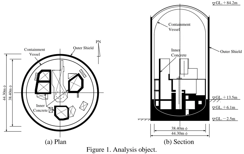
The main plan and section of the 3 loop PWR type reactor building which is dealt with in this study are shown in Fig. 1. The diameter of the circular basemat is 44.3 m, the basemat height is 8.6 m, and the height of the reactor building including the basemat is about 90 m.
The shear wave velocity of the ground is Vs = 2200 m/s near the ground surface. The ground deeper than about 70m is slightly harder and the shear wave velocity is Vs = 2560 m/s. Since the ground surface level around the building is GL. +13.5 m and the basemat bottom level is GL. -2.5 m, the embedding depth is 16.0 m, as shown from the section in Fig. 1. The surrounding soil is a rock with Vs = 2200 m/s, and there is no waterproof layer between the surrounding soil and the building.
PN
44
.30
m
φ
38
.40
m
φ
Containment Vessel
Inner Concrete
Outer Shield
GL.+13.5m
GL.+6.1m
GL.-2.5m
38.40mφ
44.30mφ
Containment Vessel
Outer Shield Inner
Concrete
GL.+84.2m
(a) Plan (b) Section
Figure 1. Analysis object.
Soil spring model
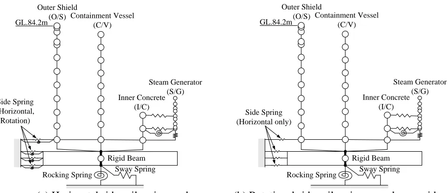
As shown in Fig. 2, the soil spring model consists of a lumped-mass basemat, basemat bottom soil springs and side soil springs. According to JEAG (1991), the stiffness of the bottom soil spring is set by the value of the real part of the soil impedance at the frequency of zero, and the stiffness of the side soil spring is set by the maximum value of the real part of the soil impedance. The impedance of the former is evaluated by vibration admittance theory by Tajimi (1952) and the latter impedance is evaluated by the Novak et al. (1978). Damping of the bottom and the side soil springs are evaluated from the imaginary part of the impedance at the first basemat mode.
Outer Shield
(O/S) Containment Vessel (C/V)
Inner Concrete (I/C)
Steam Generator (S/G) GL.84.2m
Rigid Beam Sway Spring Rocking Spring
Side Spring (Horizontal,
Rotation)
Outer Shield
(O/S) Containment Vessel (C/V)
Inner Concrete (I/C)
Steam Generator (S/G) GL.84.2m
Rigid Beam Sway Spring Rocking Spring
Side Spring (Horizontal only)
(a) Horizontal side soil springs only (b) Rotational side soil springs are also considered Figure 2. Soil spring model.
3-D FE soil model
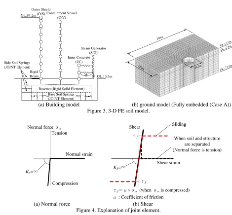
As shown in Fig. 3(a), for the 3-D FE soil model, the building model is the same lumped-mass stick model as the soil spring model, the basemat is modelled by solid elements, and it is assumed to be rigid considering the constraining effect of the upper building.
Fig. 3(b) shows the ground model of the 3-D FE soil model, which is modelled by solid elements. To prevent the influence of the building model on the ground behavior near the ground model boundary, the ground is modelled up to about 5 times of the building basemat width in a plane, and GL. -73.5m where the physical property value of the ground changes in depth. The mesh size of the ground model is set to be at least 4 meshes per wavelength in order to secure analysis resolution up to around 50 Hz. Specifically, the size of the mesh is set to be 2200/50/4 = 11m or less at the maximum. On the side of the ground model, a shear column is installed to simulate the semi-infinite ground, and it is connected with the ground model with a damper. Also, a viscous boundary is set on the bottom of the ground model. In order to save analysis time, a 1/2 model considering symmetric conditions is adopted.
The building and the ground are connected with joint elements so that separating and contact phenomena could be taken into consideration on both the basemat bottom and side. As shown in Fig. 4, the stiffness of the joint element is rigid while the building and ground are contacting (compression) and becomes zero in both axial and shear directions while they are separating (tension). The stiffness in the shear direction can be made zero when the shear force exceeds the frictional resistance (= coefficient of friction × axial force).
Since the basemat consists with solid elements, the basemat model and the ground model can be connected by the joint element directly. On the other hand, for the lumped-mass stick model, as shown in Fig. 3(a), a rigid beam is set from the mass point of the building model to the ground model, and connected the node of the ground model and the end point of the rigid beam with the joint element.
pressure on the side surface of the building is obtained by self-weight analysis of the surrounding soil only, assuming the surrounding soil is buried back.
GL.13.5m Outer Shield
(O/S) Containment Vessel (C/V)
Inner Concrete (I/C)
Steam Generator (S/G)
Rigid Beam GL.84.2m
Basemat(Rigid Solid Element)
… …
Side Soil Springs (JOINT Element)
Base Soil Springs (JOINT Element)
240m
120
m 44.3m
GL.13.5m
GL.-2.
5m
GL.-73
.5m
(a) Building model (b) ground model (Fully embedded (Case A))
Figure 3. 3-D FE soil model.
Tension
Compression Kn=∞
Normal force σn
Normal strain
KS=∞
When soil and structure are separated (Normal force is tension) Shear
Shear strain τf
τf
τf=μ×σn (when σn is compressed) Sliding
μ : Coefficient of friction
(a) Normal force (b) Shear
Figure 4. Explanation of joint element.
Input seismic motion
0.02 0.1 1 5 30
20
10
0
h=0.05
Period (s)
Acceleration
(m
/s
2)
80 60
40 20
0 10
0
-10
MAX.= 8.5m/s2
Time (s)
Accel
. (
m
/s
2)
(a) Acceleration time history (b) Acceleration response spectrum
Figure 5. input seismic motion on basemat bottom level of GL. -2.5 m.
COMPARISONS OF RESPONSE ANALYSIS RESULTS BY DIFFERENCE OF MODELLING
Soil impedance
Soil impedances of the side soil is evaluated for the soil spring model and the 3-D FE soil model mentioned above.
The soil impedance of the soil spring model is evaluated by the Novak’s formula.
On the other hand, for the 3-D FE soil model, the soil impedance is evaluated as the reciprocal of the average displacement obtained by applying unit force into a rigid basemat on the 3-D FE soil model as shown in Fig. 6. When a load is applied into the rigid basemat whose shape is as shown in Fig. 6, the soil impedance combined with the side soil and the bottom soil is evaluated. Therefore, the soil impedance of the side soil is evaluated by subtracting the soil impedance of the bottom soil from that of the entire basemat. Furthermore, when there is a waterproof layer between the side soil and the building, it may be considered that the building and the side soil behave independently (slide freely) in the shear direction. The soil impedance is also evaluated for the case where the basemat and the side soil behave independently in the shear direction.
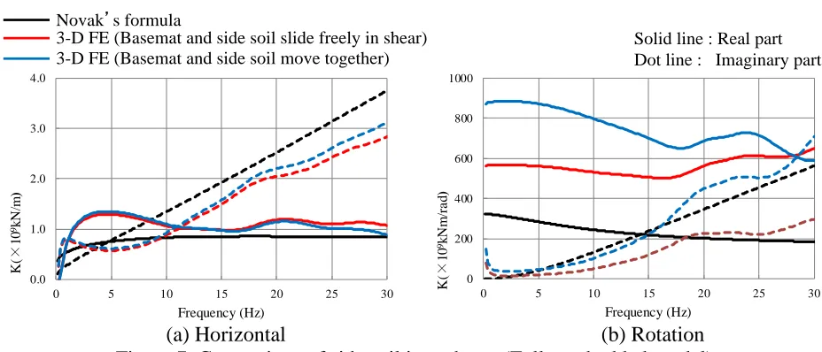
Fig. 7 shows that the soil impedance by the 3-D FE soil model is substantially consistent with the result of Novak’s formula in the horizontal direction. On the other hand, the following two findings can be respect to the rotational direction. First, the soil impedance in the rotational direction is a relatively large value even when the building and the side soil slide freely in the shear direction. In other words, it is better to consider not only the horizontal side soil spring but also the rotational side soil spring for the soil spring model. Secondly, in the 3-D FE soil model, the case of considering the slide in the shear direction is closer to the result of Novak’s formula. This is because the rotational spring of Novak’s formula is originally evaluated by the cumulative evaluation of the rotation per unit depth. Therefore, it is considered that it gives a rather small result as rigidity (that is the real part of the impedance) than that obtained from the rotational behaviour of the whole building.
Unit horizontal distributed load
Average horizontal deformation
Rotational deformation Unit rotational load
(a) Horizontal (b) Rotation (building and soil move together)
Novak’s formula
3-D FE (Basemat and side soil slide freely in shear) 3-D FE (Basemat and side soil move together)
Solid line : Real part Dot line : Imaginary part
0.0 1.0 2.0 3.0 4.0
0 5 10 15 20 25 30
K(
×
10
9kN
/m
)
Frequency (Hz)
0 200 400 600 800 1000
0 5 10 15 20 25 30
K(
×
10
9k
N
m
/r
a
d
)
Frequency (Hz)
(a) Horizontal
(b) Rotation
Figure 7. Comparison of side soil impedance (Fully embedded model)
Natural Frequency
Table 1 shows natural frequencies evaluated for the above mentioned analysis models.
As regards the soil spring model, the natural frequency is slightly higher when the rotational side soil spring is taken into consideration, and the natural frequency is slightly lower in the case where the building and the side soil slide freely in the shear direction in the 3-D FE soil model. Comparing the soil spring model and the 3-D FE soil model, the former’s natural frequency is slightly lower than the latter’s, but the difference is small. This is thought to be due to the fact that the side soil impedance by the 3-D FE soil model is stiffer than Novak’s formula, although there is the influence of the soil impedance of the basemat bottom. As a result, in the soil spring model, it is close to the result of the 3-D FE soil model in which the building and the side soil slide freely in the shear direction when considering the rotational side soil spring.
Table 1:
Comparison of natural frequency (Hz)
.Mode
Soil spring model 3-D FE soil model
Only horizontal spring is considered
Both horizontal and rotational spring are considered
Building and soil move together (No sliding)
Building and soil slide freely in shear
1st 3.698 3.773 3.865 3.748
2nd 5.322 5.328 5.341 5.338
3rd 6.819 6.821 6.832 6.831
4th 10.44 10.45 10.54 10.52
Analysis cases
For the 3-D FE soil model, as shown in Table 2, the parameters for investigating the degree of influence are the consideration of contact and separating and the friction coefficient, and three cases are conducted. Case 1 is a case where the building and the side soil move together completely (no sliding), and corresponds to Fig. 6(b) in investigation of the soil impedance. Cases 2 and 3 are set with the friction coefficient between the side soil and the building as a parameter. As an extreme example, the case where the friction is zero (the building and the side soil is always sliding freely even when they are in contact) and infinity (the building and side soil always move together, regardless of how much the shear force increases) is performed.
Table 2:
Analysis cases for 3-D FE soil model
.Parameter for joint element
Contact and separation Coefficient of friction
Case 1 Not considered -
Case 2 Considered ∞ (No sliding)
Case 3 ↑ 0 (Sliding freely)
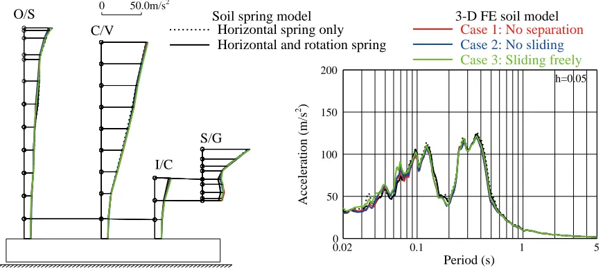
Seismic responses
The results of applying the seismic wave into each analysis model are shown in Fig. 8 for the maximum acceleration response, Fig. 9 for the response spectrum and Table 3 for the basemat uplift ratio.
Fig. 8 and Fig. 9 show that the influence of the analysis model and modelling difference between the building and the side soil on both the maximum response and the response spectrum is very small.
The basemat uplift ratio decreases as the degree of fixation between the building and the surrounding soil becomes weak. Particularly in the case of the soil spring model with only the side horizontal soil springs, the uplift ratio is extremely low, and It becomes smaller than that of the 3-D FE soil model which the building and the side soil slide freely.
0.02 0.1 1 5
200
150
100
50
0
h=0.05
Period (s)
A
cceleration
(
m
/s
2 )
Case 1: No separation
Case 2: No sliding
Case 3: Sliding freely
3-D FE soil model Horizontal spring only
Horizontal and rotation spring Soil spring model
0 50.0m/s2
O/S
C/V
I/C
S/G
Figure 8. Maximum acceleration response Figure 9. Horizontal floor response spectra
Table 3: Comparison of basemat uplift ratio (%).
Soil spring model 3-D FE soil model
Horizontal spring only
Horizontal and
rotation Case 1: No separation
Case 2: No sliding (friction is infinity)
Case 3: Sliding freely (no friction)
31.9 71.7 99.4 71.3 53.2
EFFECT ON EMBEDDED AREA
Analysis cases
In the actual site, there are the steps in basemat level, the adjacent building and so on, and it is rare that the building is entirely embedded in the surrounding soil. Therefore, using the 3-D FE soil model described in above, the following cases are examined with reference to the situation of the site where the target building actually exists.
Case A: The entire circumference of the building is embedded (Fully embedded) Case B: 3/4 of the whole is embedded
Case C: About half of the whole is embedded
Case D: The entire circumference is embedded but a part of it is an adjacent building
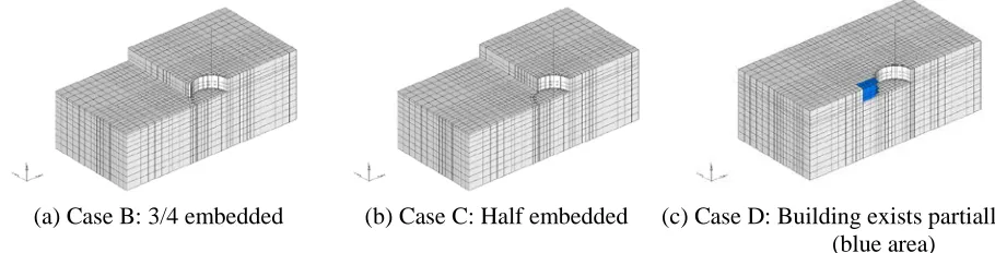
In addition to the case A of fully embedded shown in Fig. 3(b), an analysis models for case B to D are shown in Fig. 10. It is necessary to set the position of the non-embedded part or the adjacent building against the excitation direction for the case B to D, but since the ground model is 1/2, these parts are modelled so as to be symmetrical with respect to the axis of symmetry to affect the response most.
In the case D, it is assumed that the adjacent building (the blue painted part in the figure) is combined with the target building, and its boundary with the soil is the same as the boundary between the target building and the soil. Where, the adjacent building is a two-layer building consisting of a wall and a floor, and it is modelled by a shell element. That is, it has a building with a space inside.
(a) Case B: 3/4 embedded (b) Case C: Half embedded (c) Case D: Building exists partially
(blue area) Figure 10. Analysis model for difference of embedded area
Natural frequency
Table 4: Comparison of natural frequency (Hz). (3-D FE soil model)
Mode Case A: Fully embedded Case B: 3/4 embedded Case C: Half embedded Case D: Building exists partially
1st 3.865 3.822 3.804 3.841
2nd 5.341 5.335 5.332 5.339
3rd 6.832 6.828 6.826 6.831
4th 10.54 10.52 10.52 10.53
Soil impedance
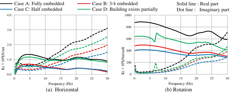
For the four 3-D FE soil models with different embedding conditions shown in the above, the soil impedance for the side soil is evaluated by the method shown in Fig. 6.
The results are shown in Fig. 11. Although the soil impedance decreases as the embedding area gets smaller, the difference between 3/4 embedded and half embedded is small when compared with the difference between fully embedded and 3/4 embedded. On the other hand, when a part of the soil is replaced with an adjacent building, the impedance of the rotational component is discontinuous around 6.5 Hz. This phenomenon seems to be caused by an effect with a building replacing a part of the soil. This is because when the primary frequency in the vertical direction is evaluated from the mass and the rigidity of the adjacent building, it is approximately 6.5 Hz.
Case A: Fully embedded Case B: 3/4 embedded
Case C: Half embedded Case D: Building exists partially
Solid line : Real part Dot line : Imaginary part
0.0 1.0 2.0 3.0 4.0
0 5 10 15 20 25 30
K(
×
10
9kN
/m
)
Frequency (Hz)
0 200 400 600 800 1000
0 5 10 15 20 25 30
K(
×
10
9k
N
m
/r
a
d
)
Frequency (Hz)
(a) Horizontal (b) Rotation
Figure 11. Comparison of side soil impedance (effect on embedded area).
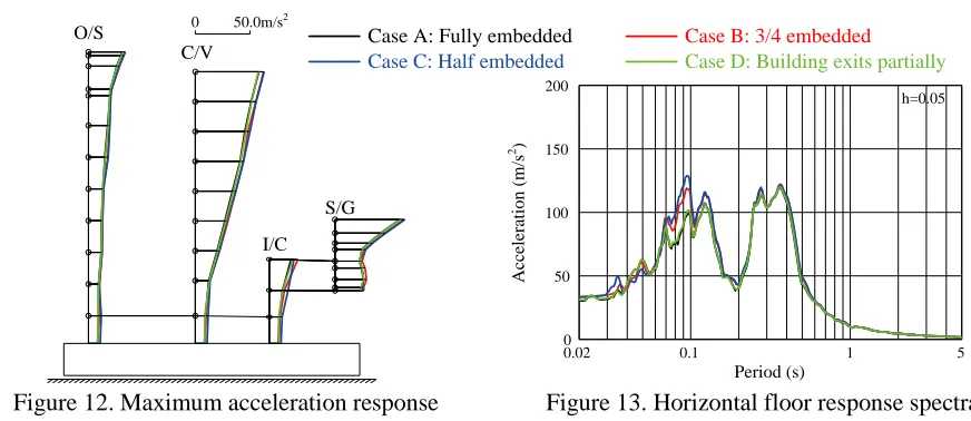
Seismic responses
The results of applying the same seismic waves into each analysis model are shown in Fig. 12 for the maximum acceleration response, Fig. 13 for the response spectrum and Table 5 for the basemat uplift ratio.
Fig. 12 and Fig. 13 show that the influence of the embedded range and the presence of adjacent building on both the maximum response and the response spectrum is very small.
0.02 0.1 1 5 200
150
100
50
0
h=0.05
Period (s)
Acceleration
(m
/s
2)
O/S
C/V
I/C S/G
0 50.0m/s2
Case A: Fully embedded Case B: 3/4 embedded
Case C: Half embedded Case D: Building exits partially
Figure 12. Maximum acceleration response Figure 13. Horizontal floor response spectra
(O/S dome top)
Table 5: Comparison of basemat uplift ratio (%). (3-D FE soil model)
Case A: Fully embedded Case B: 3/4 embedded Case C: Half embedded Case D: Building exists partially
71.3 65.1 57.4 71.3
CONCLUSION
The modelling method of side soil for the embedded nuclear power plant facilities is examined. As a result, the following findings are obtained.
In the case of the 3-D FE soil model,the horizontal responses of the building are hardly affected by the contact and separation in the axial direction and the friction in the shear direction between the side soil and the building. However, these affect the magnitude of the basemat uplift ratio. Similarly, the difference in the range of embedding and the presence of adjacent building also have little influence on the horizontal responses.
For the soil spring model as well, the difference in modelling of the side soil has little influence on the horizontal response of the building, and these horizontal responses almost match the 3-D FE soil model. When the rotational side soil spring is not taken into consideration in the soil spring model, the basemat uplift ratio becomes extremely small, and it is rather consistent with the result of the 3-D FE soil model when considering the rotational side soil spring.
From the above mentioned findings, it is confirmed that it is more appropriate to model the soil spring model as considering the rotational side soil spring even if the embedded state is incomplete to some extent in consideration of the actual situation of the site.
REFERENCES
Japan Electric Association Guideline (JEAG (1991)), “Technical Guidelines for Aseismic Design of Nuclear Power Plants - JEAG 4601-1991 Supplement” (in Japanese)
Novak, M., Nogami T. and Aboul-Ella F. (1978), “Dynamic Soil Reactions for Plane Strain Case”, The Journal of the Engineering Mechanics Division, ASCE, 104(4), 953-959.