ABSTRACT
GUO, XIANGYANG. A Study of Code Compilation and Garbage Collection on Android. (Under the direction of Dr. Huiyang Zhou).
Nowadays, Android systems are the most widely used platform for mobile devices. Numerous apps have been developed and deployed on Android systems. As a result, the efficiency of both the code and the runtime memory management, i.e., garbage collection (GC), running on Android devices has huge impact on user experience and the battery life. A detailed study on code compilation and GC on Android is presented in this thesis.
A Study of Code Compilation and Garbage Collection on Android
by Xiangyang Guo
A thesis submitted to the Graduate Faculty of North Carolina State University
in partial fulfillment of the requirements for the degree of
Master of Science
Computer Engineering
Raleigh, North Carolina 2016
APPROVED BY:
_______________________________ Dr. Huiyang Zhou
Committee Chair
_______________________________ _______________________________
ii DEDICATION
iii BIOGRAPHY
iv ACKNOWLEDGMENTS
I would like to thank Dr. Huiyang Zhou for being my advisor since I joined North Carolina State University. I am thankful to his persistent guidance, discussions and suggestions. I would also like to thank Dr. Byrd and Dr. Tuck for serving on my thesis committee and all the feedback of my work.
I would like to thank all my colleagues: Yi, Ping, Chao, Hongwen, Mayank, Yuan, Qi and Zhen for their discussions and feedback.
v TABLE OF CONTENTS
LIST OF TABLES ... vi
LIST OF FIGURES ... vii
1 Introduction ... 1
2 Backgrounds ... 5
2.1 Android Basics ... 5
2.2 Code Compilation in ART ... 7
2.3 Garbage Collection in ART ... 11
3 ART Compiler Study ... 13
3.1 Case Study: Fibonacci Sequence ... 13
3.2 Dalvik Bytecode Optimizer ... 21
3.2.1 Compiler Frontend ... 22
3.2.2 Compiler Backend ... 31
3.3 Experiment Results ... 40
4 ART GC Study ... 50
4.1 Case Study: Camera App ... 53
4.2 New GC Selection Algorithm ... 54
4.3 Experiment Results ... 55
5 Related Work ... 59
6 Conclusion ... 62
vi LIST OF TABLES
Table 1. Comparison of Java bytecode and Dalvik bytecode ... 9
Table 2. Representation of types in Dalvik bytecode [20]... 23
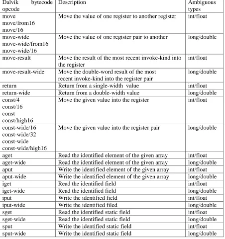
Table 3. Dalvik bytecode instructions with ambiguous types ... 24
Table 4. Intrinsic functions of ‘iput’ ... 30
Table 5. Descriptions of benchmarks ... 41
vii LIST OF FIGURES
Figure 1. Android Architecture [7] ... 6
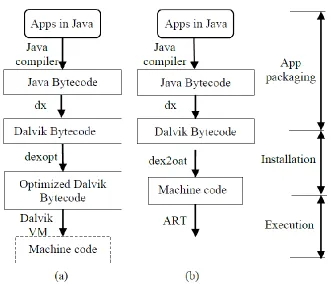
Figure 2. Android app compilation (a) JIT (b) AOT ... 8
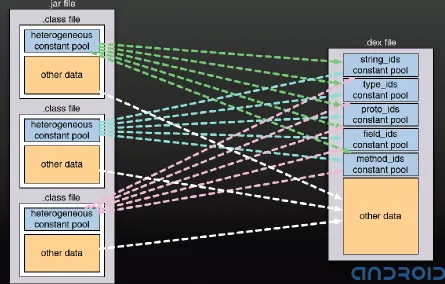
Figure 3. Compilation Process from Java bytecode to Dalvik bytecode [5] ... 9
Figure 4. Java code of Fibonacci numbers ... 13
Figure 5. Dalvik bytecode of Fibonacci numbers ... 14
Figure 6. ARM assembly code for array initialization and loop branch ... 17
Figure 7. ARM assembly code for the loop body ... 19
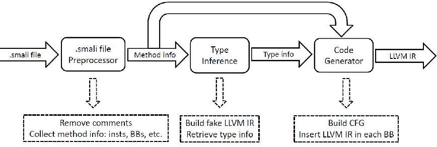
Figure 8. Framework of Dalvik bytecode optimizer ... 22
Figure 9. Framework of customized frontend ... 31
Figure 10. Standard pipeline of LLVM backend ... 33
Figure 11. Examples of describing registers with TableGen ... 34
Figure 12. Examples of describing instruction set with TableGen ... 35
Figure 13. Examples of describing calling conventions with TableGen ... 36
Figure 14. Framework of customized backend ... 38
Figure 15. Optimized Dalvik bytecode of Fibonacci numbers ... 39
Figure 16. Performance speedup on Android 5 ... 41
Figure 17. Dalvik bytecode of Boolean negation without optimization ... 42
Figure 18. ARM Assembly of Boolean negation generated on Android 5 ... 42
Figure 19. Dalvik bytecode of Boolean negation with optimization ... 42
Figure 20. Dalvik bytecode of the recursion function in benchmark 'Method' ... 44
viii
Figure 22. Comparison of performance on Android 5 and Android 6... 46
Figure 23. Performance speedup on Android 6 ... 46
Figure 24. ARM assembly generated on Android 6 from the example in Figure 17 ... 47
Figure 25. Java code of Boolean negation inside a loop... 47
Figure 26. Dalvik bytecode generated from the example in Figure 25 ... 48
Figure 27. ARM assembly generated on Android 6 from the example in Figure 26 ... 48
Figure 28. Algorithm for next GC type selection ... 51
Figure 29. GC activities of Camera app... 53
Figure 30. Heap usage of the Camera app to show GC activities ... 54
Figure 31. Optimized algorithm for next GC type selection ... 55
Figure 32. Pause time comparison on Android 5 (the lower the better) ... 56
1 1 Introduction
With the rapid growth of smartphones, the number of mobile computing devices surpassed the number of personal computers (PCs) in 2014[13]. The number of smartphone users reaches 1.75 billion in 2014 [14] and is expected to increase to 2.5 billion by 2015[16]. Among these smartphones, the majority use the Android systems, 81.1% in 2014[15]. Making use of such ubiquitous computing devices, numerous Android applications (apps) have been developed and deployed. As a result, it is crucial to examine how efficiently the apps are executed on Android systems. Given the massive number of Android devices, even a small improvement will lead to huge impacts on the user experience and battery life.
In this thesis, both code compilation and memory management in Android systems are studied to understand the constraints of mobile devices, to evaluate both the code generated by the static compiler and memory management by the runtime garbage collection (GC), and to identify opportunities to improve them.
2 the app runs. Therefore, it can achieve higher performance and improves the battery life at the cost of longer installation time. As Dalvik bytecode is a more compact representation than the native binary, one potential drawback of the ART system is the app’s code size and the resulting pressure on the instruction cache.
Besides Java, another way to develop Android apps is to use the C/C++ programming language through the Java native interface (JNI). However, as cautioned in Android developers’ guide [18], this approach incurs substantial complexity and may lose portability
across different devices.
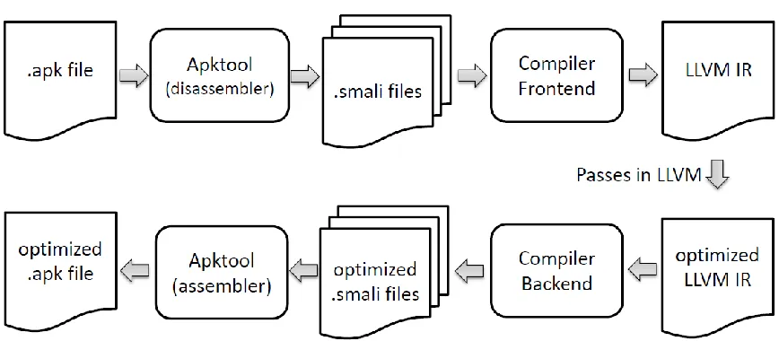
3 In this thesis, an empirical study on both code compilation and runtime memory management are performed on the Android 5 system. The analysis shows the following key observations: (1) The constraints of current mobile devices limit how aggressive the compiler optimizes the code. As a result, the code generated in Android systems is not highly optimized. (2) The current GC selection algorithm cannot always select the collector with the best efficiency. (3) There exist good opportunities to optimize Android for more efficient execution. A Dalvik bytecode optimizer based on LLVM framework is implemented to optimize Dalvik bytecode. It can extract the Dalvik bytecode from the Android application package, convert the Dalvik bytecode into LLVM intermediate representation (IR), apply optimization passes, transfer the LLVM IR back to Dalvik bytecode and pack it as a new Android application package. This way, an optimized app can be achieved without additional optimization passes on Android smartphone. Therefore, the app installation time is not affected while the execution time can be significantly reduced. The experimental results show that the optimizer improves the performance significantly on a Nexus 5 smartphone running on Android 5 and the latest Android 6. An optimization on the GC selection algorithm is also proposed, which fixes the pathological cases of the current algorithm and can reduce the pause time significantly for a range of apps.
5 2 Backgrounds
2.1 Android Basics
Android systems contain several key components as shown in Figure 1 [7]: Linux kernel, Libraries, Android Runtime, Application Framework and Applications.
Android systems are built on Linux kernel with customized modifications and enhancements because of the unique features and requirements of smartphones. For example, Android systems implement and apply customized Inter Processes Communication (IPC) named Binder in order to achieve low processing overhead and high security. Because smartphones are powered by batteries that usually have limited capacity, the Linux kernel in Android systems has an enhanced Power Management (PM), which uses more aggressive power management policies. For instance, the PM provides the ‘weak lock’, which can be requested by applications to keep the devices power on.
In terms of Libraries, Android systems also imply some unique features. For example, instead of inheriting the traditional libc library, Android systems implement a customized libc called bionic. The bionic library is implemented and optimized for embedded systems because of its smaller size and fast code paths. The Libraries contain rich native libraries targeting different usages: WebKit for web browsers usage, Media Framework for processing videos and audios, a light-weight SQLite for data storage, Surface Manager for rendering surface to framebuffer, OpenGL ES for rendering 3D graphics, SSL for internet security, FreeType for font rendering and so on.
6 structures, file accesses and so on. Before Android 5, the DVM is used by default and it runs Dalvik Bytecode using interpreter or JIT.
Figure 1. Android Architecture [7]
Since Android 5, a new Android Runtime ART is used by default. It compiles the Dalvik bytecode into native code and executes native code directly instead of using interpreter or JIT. In this way, it can achieve better performance and power efficiency.
7 System is used to show different views (e.g. text, buttons, bars and so on) to implement user interface.
2.2 Code Compilation in ART
8 Figure 2. Android app compilation (a) JIT (b) AOT
9 Figure 3. Compilation Process from Java bytecode to Dalvik bytecode [5]
Similar to Java bytecode, Dalvik bytecode is defined upon a virtual machine to achieve portability among different devices. One key difference is that the Dalvik virtual machine uses a load-store style register-based RISC instruction set architecture (ISA) while Java virtual machine is based on a stack-based ISA. A detailed comparison of Java bytecode and Dalvik bytecode is shown in Table 1 [9].
Table 1. Comparison of Java bytecode and Dalvik bytecode
Java Bytecode Dalvik Bytecode
Application Structure multiple .class files single .dex file
Register architecture stack-based register-based
Instruction set 200 instructions 218 instructions
Constant pool structure multiple constant pools single constant pool
Ambiguous primitive types no yes
10 Dalvik bytecode is a register-based load-store style ISA with variable-length encoding. It is designed to achieve device portability and code size efficiency. Encoded as one or more 16-bit units, an instruction has an 8-bit opcode and variable-length operands. Current Dalvik bytecode instruction set defines operations for opcode values ranging from 0x00 to 0xE2. The remaining ones, from 0xE3 to 0xFF are currently unused. Each opcode is associated with a specific format for operand encoding. For example, a move instruction with the opcode as 0x04 uses a format of ‘12x’, which means that it uses two 4-bit virtual register operands, i.e., move
RA, RB, where A and B are 4-bit numbers. In comparison, a move instruction with the opcode as 0x05 uses a format of ‘22x’, which means that the instruction has a destination virtual register operand with 8-bit encoding and a source virtual register operand with 16-bit encoding, i.e., move/from16 RAA, RBBBB, where AA is an 8-bit value and BBBB is a 16-bit value. As a result, an instruction with the format of ‘move RA, RB’ has a size 16 bits while an instruction with the format of ‘move RAA, RBBBB’ has a size of 32 bits. The reason for such
variable-length encoding for operands is that most methods do not use a large number of register operands and fixed-length encoding leads to a waste in the application package (apk) space.
11 2.3 Garbage Collection in ART
ART relies on the garbage collection (GC) runtime to manage memory automatically. It applies different types of collectors in different situations. The SS collector divides the allocation space into two. The app can only allocate objects in one space. When the GC is triggered, it moves the live objects from one space to the other. The dead objects left in the previous space will be reclaimed. Then, the roles of these two spaces are swapped. The SS collector can reduce fragmentation by moving live objects next to each other. As copying objects is time consuming, the SS collector is only used in limited situations. For example, when a foreground app goes to background as a result of the ‘home’ button being pressed, the SS collector will be triggered to compact the heap [11]. The reason is that users do not care about the pause time in this case.
12 be allocated. There are three types of CMS collectors in ART: the full CMS collector, the partial CMS collector, and the sticky CMS collector. The full CMS collector deletes dead objects in the Zygote Space, Malloc Space and Large Object Space while the partial CMS collector deletes dead objects in the Malloc Space and Large Object Space. In comparison, the sticky CMS collector only removes dead objects among those which were allocated since the last GC iteration. To implement sticky CMS, ART maintains an allocation stack, which records the newborn objects since last GC iteration. Since sticky CMS does not need to mark the whole Malloc Space, it consumes less running time than partial CMS. Based on the assumption that most objects have very short lifetimes [24], the sticky CMS collector can delete a large amount of dead objects within little running time.
13 3 ART Compiler Study
3.1 Case Study: Fibonacci Sequence
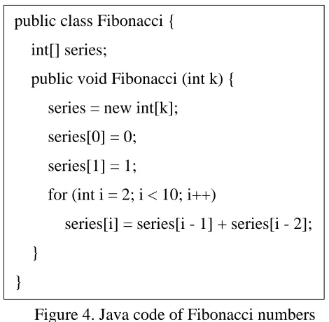
In this section a microbenchmark that computes Fibonacci numbers is used to analyze Android code compilation. Both the Dalvik bytecode and native machine code are analyzed to evaluate the code quality, understand the constraints facing the compilers for mobile devices, and identify opportunities for improvement. Here, the algorithm is implemented by using a simple array-based approach, as shown in Figure 4. The Java code in Figure 4 computes the first ten Fibonacci numbers. It first allocates the memory for the array containing the Fibonacci numbers. It initializes the first two Fibonacci numbers and then pre-computes the next eight ones in the loop.
Figure 4. Java code of Fibonacci numbers
The code is constructed for several reasons. First, the value of the input number k is not checked deliberately before accessing array elements. This way, if there is no array
public class Fibonacci { int[] series;
public void Fibonacci (int k) { series = new int[k];
series[0] = 0; series[1] = 1;
for (int i = 2; i < 10; i++)
series[i] = series[i - 1] + series[i - 2]; }
14 bound/range checking, a buffer overflow may occur. Second, the array accesses ‘series[0]’ and ‘series[1]’ by using constant array indices. Third, the loop has constant loop bounds.
PC : Dalvik bytecode instruction ; Comment 0x0000: const/4 v3, #+1
0x0001: const/4 v2, #+0
0x0002: new-array v1, v6, int[] // type@2321
0x0004: iput-object v1, v5, [I example.fibonacci.Fibonacci.series // field@8283 0x0006: iget-object v1, v5, [I example.fibonacci.Fibonacci.series // field@8283
0x0008: aput v2, v1, v2 ; series[0] = 0 0x000a: iget-object v1, v5, [I example.fibonacci.Fibonacci.series // field@8283
0x000c: aput v3, v1, v3 ; series[1] = 1 0x000e: const/4 v0, #+2 ; loop lower bound 0x000f: const/16 v1, #+10 ; loop upper bound 0x0011: if-ge v0, v1, +22 ; branch if i>=10 0x0013: iget-object v1, v5, [I example.fibonacci.Fibonacci.series // field@8283
0x0015: iget-object v2, v5, [I example.fibonacci.Fibonacci.series // field@8283
0x0017: add-int/lit8 v3, v0, #-1 ; i-1 0x0019: aget v2, v2, v3 ; series[i-1] 0x001b: iget-object v3, v5, [I example.fibonacci.Fibonacci.series // field@8283
0x001d: add-int/lit8 v4, v0, #-2 ; i-2 0x001f: aget v3, v3, v4 ; series[i-2] 0x0021: add-int/2addr v2, v3
0x0022: aput v2, v1, v0 ; series[i] = series[i-1] + series[i-2] 0x0024: add-int/lit8 v0, v0, #+1 ; i++ 0x0026: goto -23
0x0027: return-void
15 Next, the Dalvik bytecode generated from the Java code in Figure 4 is examined. The Java code is first complied into Java bytecode by the Java compiler, javac. Then the Dalvik bytecode generator dx transfers the Java bytecode into Dalvik bytecode. The Android SDK and JDK6 are used as suggested on the Android developer website to develop the apps. The resulting Dalvik bytecode of function Fibonacci is shown in Figure 5.
Several observations can be made from Figure 5. First, as mentioned in [19], the storage unit in the instruction stream is 16-bit quantity. From the instruction addresses, most Dalvik bytecode instructions have a size of either one 16-bit unit, e.g., add-int/2addr v2,v3 at address 0x0021, or two 16-bit units, e.g., add-int/lit8 v3,v0, #-1 at address 0x0017. As a result, the code size is effectively reduced. Second, there are semantically rich instructions defined in the Dalvik bytecode for instance field access and array accesses. For example, the ‘iget’ instruction can read value from one instance field while the ‘iput’ instruction can update an instance field. The ‘aget’ instruction can read the value of one element from an array while the ‘aput’
instruction can write value to one element of one array. Based on the different types of instance field and array element, different suffixes are appended to ‘iget’, ‘iput’, ‘aget’ and ‘aput’. For example, the ‘iput-object’ instruction at address 0x0004 is used to update the specific instance
16 instruction at address 0x0013, 0x0015 and 0x001b respectively. In the loop body, the virtual register v1 is used to store the instance field ‘series’ and never be redefined again. So the other two loads for instance field ‘series’ are redundant if the code can reuse v1. However, neither Common Subexpression Elimination (CSE) nor Global Value Numbering (GVN) is performed to eliminate the redundant instance field accesses. It is expected as the Java compiler at the build time, javac, does not optimize the code significantly and Java relies on the JIT compiler, a part of the Java Virtual Machine (JVM), to translate and optimize the code upon the target device. Fourth, the loop structures are implemented using a loop-bound-checking forward-jumping conditional branch together with a backward-forward-jumping ‘goto’ instruction. Apparently it is not as efficient as using a loop-bound-checking backward-jumping conditional branch.
The Dalvik bytecode will go through a program, dexopt, in Android systems when the app is installed. The dexopt mainly verifies the bytecode and optimizes it at the method level, such as method inlining or empty method removal. It does not affect the bytecode example in Figure 5. As discussed in Section 2, ART is the new compilation framework in Android systems. When an app is installed on a device, the AOT compiler dex2oat compiles the app into the native ISA code for this particular device. We use the tool ‘oatdump’ to disassemble
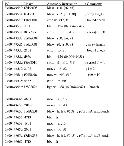
17 Among the instructions shown in Figure 6, before using the store instruction at address 0x004495ce to initialize the array element ‘series[0] = 0’, there are several instructions used for array bound/range check. The first of them, ‘ldr.w r12, [r10, #8]’ retrieves the array length
PC : Binary Assembly instruction ; Comments 0x004495c0: f8d6a008 ldr.w r10, [r6, #8]
0x004495c4: f8dac008 ldr.w r12, [r10, #8] ; array length 0x004495c8: f1bc0f00 cmp.w r12, #0 ; bound check 0x004495cc: d93f bls +126 (0x0044964e)
0x004495ce: f8ca700c str.w r7, [r10, #12] ; series[0] = 0 0x004495d2: f8d6a008 ldr.w r10, [r6, #8]
0x004495d6: f8da0008 ldr.w r0, [r10, #8] ; array length 0x004495da: 2801 cmp r0, #1 ; bound check 0x004495dc: d93c bls +120 (0x00449658)
0x004495de: f8ca8010 str.w r8, [r10, #16] ; series[1] = 1 0x004495e2: 2502 movs r5, #2 ; i = 2
0x004495e4: f04f0a0a mov.w r10, #10 ; r10 = 10 0x004495e8: 4555 cmp r5, r10
0x004495ea: f280802a bge.w +84 (0x00449642) ; branch ….
0x0044964e: 4661 mov r1, r12 0x00449650: 2000 movs r0, #0
0x00449652: f8d9e238 ldr.w lr, [r9, #568] ; pThrowArrayBounds 0x00449656: 47f0 blx lr
0x00449658: 1c01 mov r1, r0 0x0044965a: 2001 movs r0, #1
0x0044965c: f8d9e238 ldr.w lr, [r9, #568] ; pThrowArrayBounds 0x00449660: 47f0 blx lr
18 information, which is set during the array allocation function call. Then, the subsequent ‘cmp.w’ and ‘bls’ instructions check whether the arrange length is less than or equal to the
index value, the constant 0 in this case. If so, the branch at 0x004495cc will be taken and an array bound exception will be thrown using the instructions between address 0x0044964e and 0x00449656. Such a bound check may be considered necessary in this case as we intentionally did not perform any check on the array size in the Java code in Figure 4. However, after initializing the array element ‘series[0]’, the next few instructions initialize the element ‘series[1]’. In the same way, the array bound is checked again with the index value, the constant
1 this time. Between these two array bound checks, the first one is redundant as we can infer the results from the second one (i.e., if array length > 1, then array length > 0). In addition, the array length is loaded twice (0x004495c4 and 0x004495d6), although the destination register r12 of the first load has not been altered. In other words, the second bound check can use r12 directly to remove one redundant instruction. The loop branch in Figure 6 are a direct translation from the corresponding bytecode in Figure 5.
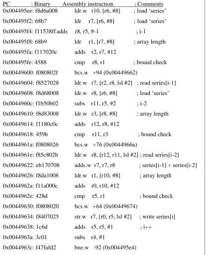
19 other words, every array access in each loop iteration involves a bound check. In this loop body, there are 24 instructions and 9 of them (i.e., 37.5%) are used for bound checking.
PC : Binary Assembly instruction ; Comments 0x004495ee: f8d6a008 ldr.w r10, [r6, #8] ; load ‘series’
0x004495f2: 68b7 ldr r7, [r6, #8] ; load ‘series’ 0x004495f4: f11538ff adds r8, r5, #-1 ; i-1
0x004495f8: 68b9 ldr r1, [r7, #8] ; array length 0x004495fa: f117020c adds r2, r7, #12
0x004495fe: 4588 cmp r8, r1 ; bound check 0x00449600: f080802f bcs.w +94 (0x00449662)
0x00449604: f8527028 ldr.w r7, [r2, r8, lsl #2] ; read series[i-1] 0x00449608: f8d68008 ldr.w r8, [r6, #8] ; load ‘series’ 0x0044960c: f1b50b02 subs r11, r5, #2 ; i-2
0x00449610: f8d83008 ldr.w r3, [r8, #8] ; array length 0x00449614: f1180c0c adds r12, r8, #12
0x00449618: 459b cmp r11, r3 ; bound check 0x0044961a: f0808026 bcs.w +76 (0x0044966a)
0x0044961e: f85c802b ldr.w r8, [r12, r11, lsl #2] ; read series[i-2]
0x00449622: eb170708 adds.w r7, r7, r8 ; series[i-1] + series[i-2] 0x00449626: f8da1008 ldr.w r1, [r10, #8] ; array length
0x0044962a: f11a000c adds r0, r10, #12
0x0044962e: 428d cmp r5, r1 ; bound check 0x00449630: f0808020 bcs.w +64 (0x00449674)
0x00449634: f8407025 str.w r7, [r0, r5, lsl #2] ; write series[i] 0x00449638: 1c6d adds r5, r5, #1 ; i++
0x0044963a: 3c01 subs r4, #1
0x0044963c: f47fafd2 bne.w -92 (0x004495e4)
20 All of them can be redundant if we perform a bound check, (array length >= loop upper bound), before the loop. Also, the same as the bound checking code in Figure 6, the array length is loaded multiple times. After studying the ART source code in AOSP for Android 4.4.4 and Android 5.0, it is found that there is one optimization to remove identical bound checks. However, if the identical ones exist across loop iterations, they are not detected. Furthermore, the current code does not leverage the logic relationship among bound checks to remove redundant ones. As for the apparently redundant loads for the array length, we found that although there is dead code elimination, it is performed within a basic block. As each bound check inserts a branch, the scope is code optimization is severely affected. Also, the code for the loop body shows that there is no loop level optimization.
There are following reasons for limited optimizations in the ART compiler. First, as the Dalvik bytecode is compiled when an app is installed on a device, the compilation/installation time is a key concern. Although the bytecode preserves much of the Java semantics, such as constants or array lengths, additional compiler passes may incur overwhelmingly long installation time, especially for low-end devices with limited CPU power. Second, the storage space on a device is another concern. The AOT compiler, dex2oat, in the Android 5.0, has a small size of 83344 Bytes. With limited disk space on mobile devices, it is difficult to accommodate a full-blown compiler like gcc.
21 array.length information are preserved in the bytecode, the installation-time compiler, dex2oat in both Android 4.4 and Android 5.0, performs limited optimizations. In particular, the resulting machine code contains a significant amount of redundant bound checking instructions as well as other redundant instructions. The code layout for loops is not highly efficient, and neither loop-level optimizations nor complex constant propagations have been observed. The machine code essentially is more or less a direct translation from the Dalvik bytecode. As a result, there exists significant room to improve this installation-time compiler. The challenge, however, is how to improve it with little overhead on the compilation time as well as the compiler binary size.
3.2 Dalvik Bytecode Optimizer
22 experience, will not increase. Figure 8 shows the framework of the proposed Dalvik bytecode optimizer.
Figure 8. Framework of Dalvik bytecode optimizer
An open source tool named Apktool [1] is used to extract Dalvik bytecode from an .apk file and repack the optimized Dalvik bytecode back to a new .apk file. It presents the Dalvik bytecode as human readable .smali file [31]. Smali/baksmali is an assembler/disassembler for dex format used by Dalvik.
3.2.1 Compiler Frontend
The Dalvik bytecode optimizer takes each .smali file as input. Before the code generator generates LLVM IR based on the Dalvik bytecode, several preprocessing steps need to be done first.
23 either integer type or float type. In addition, the operations of virtual registers with type of char, byte and short use the operations of integer. For example, ‘add-int v0, v1, v2’ can be used
to calculate the sum of two virtual registers v1 and v2 whose types are short. For the virtual registers with boolean type, Dalvik bytecode does not include the value of ‘true’ or ‘false’. Instead, it uses constant value 1 or 0 to represent ‘true’ or ‘false’. Table 2 [20] lists the legal types in Dalvik bytecode while Table 3 shows the Dalvik instructions which are type ambiguous. One thing needs to mention is that the Dalvik bytecode uses constant value 0 to represent the null reference, which means the comparison operator (e.g. ‘if-nez’) cannot distinguish between the integer and the object reference. For example, v0 can represent the reference of an object. In order to check if the object is null, one comparison instruction ‘if-nez v0, :cond_0’ can be used to check if v0 does not equal with 0. However, the same
comparison instruction can also represent a comparison between a constant integer and 0. Table 2. Representation of types in Dalvik bytecode [20]
Syntax Meaning
V void; only valid for return types
Z boolean
B byte
S short
C char
I int
J long
F float
D double
Lfully/qualified/Name; the class fully.qualified.Name
[descriptor array of descriptor, usable recursively for arrays-of-arrays
24 v1 is defined as a reference of an array object at address 0x0006 while it is redefined as an integer with value of 10 at address 0x000f.
Table 3. Dalvik bytecode instructions with ambiguous types Dalvik bytecode
opcode
Description Ambiguous
types move
move/from16 move/16
Move the value of one register to another register int/float
move-wide
move-wide/from16 move-wide/16
Move the value of one register pair to another long/double
move-result Move the result of the most recent invoke-kind into the register
int/float move-result-wide Move the double-word result of the most
recent invoke-kind into the register pair
long/double
return Return from a single-width value int/float
return-wide Return from a double-width value long/double
const/4 const/16 const
const/high16
Move the given value into the register int/float
const-wide/16 const-wide/32 const-wide
const-wide/high16
Move the given value into the register pair long/double
aget Read the identified element of the given array int/float
aget-wide Read the identified element of the given array long/double
aput Write the identified element of the given array int/float
aput-wide Write the identified element of the given array long/double
iget Read the identified field int/float
iget-wide Read the identified field long/double
iput Write the identified field int/float
iput-wide Write the identified filed long/double
sget Read the identified static field int/float
sget-wide Read the identified static field long/double
sput Write the identified static field int/float
25 In contrast, LLVM IR has strict type requirement and it is in SSA form. In order to transfer the Dalvik bytecode into LLVM IR, the first challenge is to retrieve the type information of each virtual register. Here, a context based type inference is proposed. Similar approach is used by ded decompiler [9] and dexpler [3]. The Dalvik bytecode instructions can be categorized into two categories: the first category contains the instructions whose opcode encodes the type information. For example, in Figure 5, the instruction ‘add-int/lit8 v3, v0, #-1’ at address 0x0017 defines a new virtual register v3. The opcode ‘add-int/lit8’ means the two
source operands should be a virtual register with integer type and an immediate number while the destination register should be integer type. So we can infer that v3 is in integer type just based on its opcode. Most of the computation instructions belong to this category. The second category contains instructions whose opcode has no hint of type. All the instructions in Table 3 belong to this category. The data flow information such as use-definition chain and definition-use chain can be used to detect the type information. For example, in Figure 5, the virtual register v3 is defined with value 1 at address 0x0000. However, v3 could be integer or float without the analysis of its context. Based on data flow information, v3 is used in the instruction ‘aput v3, v1, v3’ at address 0x000c. In this instruction, v3 is used twice: the first
26 v3’ because v1 represents the reference of an array object, whose type can be found when v1
is defined initially. The virtual register ‘v1’ is defined in instruction ‘iget-object v1, v5, [I example.fibonacci.Fibonacci.series // field@8283’ at address 0x0006, from which we can infer that v1 represents a one dimension array whose element is integer type. As shown in Table 2, ‘[I’ means the instance field is one dimension array with integer type.
From the above analysis, we can conclude that data flow information is critical for type inference. In order to retrieve the data flow information, we treat each virtual register as integer type and build a fake IR for each method. This fake IR is only for retrieving the data flow information such as the definition-use chain and use-definition chain. When building this fake IR, another challenge is that the Dalvik bytecode is not in SSA form while LLVM does require all virtual registers to be in SSA form. However, the memory objects are not required to be in SSA form in LLVM IR. It is recommended to make a stack variable for each mutable variable in a function [21] and then use ‘load’ and ‘store’ to access each mutable variable. For each virtual register within one method shown in the .smali file, an ‘alloca’ instruction is used to allocate memory on the stack frame. Then the ‘load’ and ‘store’ instructions are used to read and update to the virtual registers. In this way, we can get rid of creating Phi node. After building an initial LLVM IR with a lot of ‘load’ and ‘store’ instructions, an optimization pass named ‘mem2reg’, whose job is to do register promotion, is applied for eliminating the
27 of each operand is attached to each LLVM IR. With this metadata and dataflow information, we do type inference for instructions belonging to the second category.
1. For instructions whose opcode is ‘iget’,’iget-wide’, ‘iput’, ‘iput-wide’, ‘sget’, ‘sget-wide’, ‘sput’ or ‘sput-wide’ , the last operand of the Dalvik instruction shows the
type information. For example, the instruction ‘iget v5, v0, Lcom/android/cm3/LoopAtom;->FIBCOUNT:I’ reads the instance field ‘FIBCOUNT’ within the class ‘Lcom/android/cm3/LoopAtom’. The type of this
instance field is ‘I’. As mentioned in Table 2. ‘I’ represents the integer. So the virtual register v5 defined by this instruction is integer type.
2. For instructions whose opcode is ‘aget’, ‘aget-wide’, ‘aput’ and ‘aput-wide’, we need to find the producer of the array reference. One thing need to mention is that in this fake IR, if the producer of the array reference is a Phi node or a ‘move’ instruction, we need to go further to find the initial producer because neither Phi node nor ‘move’ instruction contains the type information of array. The initial producer of an array object (e.g. the formal argument, ‘new-array’ instruction, ‘iget-object’ instruction and so on) contains type information of the array element.
3. For instructions whose opcode is ‘const’ or ‘const-wide’, we need to find the users of this instruction. Similarly, the users could be Phi node or ‘move’ instruction. In
28 4. For instructions whose opcode is ‘move-result’ or ‘move-result-wide’, they follow an ‘invoke’ instruction immediately and contain the return value of the callee. The
type information can be retrieved from the callee’s signature. For example, the instruction ‘invoke-virtual {p0, v0}, Lcom/android/cm3/MethodAtom;
->arithmeticSeries(I)I’ is followed by the instruction ‘move-result v0’. From the ‘invoke’ instruction, we can find that the callee’s name is ‘arithmeticSeries’ and the return value is an integer because the last ‘I’ represents the type of return value. So
the virtual register v0 should be integer type.
5. For instructions whose opcode is ‘move’ or ‘move-wide’, either the users of this instruction or the definition of the source operand can be used to retrieve the type information.
6. For instructions whose opcode is ‘return’ or ‘return-wide’, the signature of this method can be used to decide the type of the virtual register. For example, if the instruction ‘return v0’ is used in method ‘arithmeticSeries(I)I’, we can conclude
that the v0 is an integer register.
29 As discussed in session 3.1, Dalvik bytecode includes rich instructions for instance field, static filed and array element access. Each of these complex instructions involves address calculation and load/store operation. In LLVM IR, the ‘getelementptr’ instruction is used to calculate the memory address and ‘load’/’store’ instruction is used to access certain memory address. If we translate these complex instructions strictly based on their syntax (e.g. each instruction is converted to one ‘getelementptr’ instruction following by a ‘load’/’store’
instruction), the compiler backend needs to do a lot of work to analysis and combine the corresponding ‘getelementptr’ instruction and ‘load’/’store’ instruction to convert them back to ‘iget’, ’iput’, ’aget’, ’aput’, ’sget’ or ’sput’. Fortunately, LLVM supports user to define intrinsic functions to simulate new instructions. For example, for ‘iput vA, vB, field@CCCC’
instruction, which can update value to an instance filed with integer type or float type, two intrinsic functions are defined as shown in Table 4 to update the integer value and float value respectively. The intrinsic functions three source operands: the first parameter ‘llvm_i32_ty’ or ‘llvm_float_ty’ represents the virtual register vA; the second parameter ‘llvm_i32_ty’
represents the virtual register vB, which represents an object reference; the third parameter ‘llvm_i32_ty’ represents the instance field ‘filed@CCCC’. From Figure 5, we can observe that
30 that the optimization passes can process the intrinsic function properly. ‘IntrNoMem’ means the intrinsic does not access memory or have any other side effects. ‘IntrReadArgMem’ means
the intrinsic reads only from memory that one of its argument points to. ‘IntrReadMem’ means the intrinsic reads from unspecified memory. ‘IntrReadWriteArgMem’ means the intrinsic reads and writes to memory that its argument points to.
Table 4. Intrinsic functions of ‘iput’
def int_dex_iput : Intrinsic<[], [llvm_i32_ty, llvm_i32_ty, llvm_i32_ty], [IntrReadWriteArgMem]>;
def int_dex_iput_float : Intrinsic<[], [llvm_float_ty, llvm_i32_ty, llvm_i32_ty], [IntrReadWriteArgMem]>;
Besides these intrinsic functions, we also define other intrinsic functions such as ‘array-length’, ‘new-array’, ‘new_instance’, ’check_cast’, ‘instance_of’, ‘throw’, ‘cmpl_float’, ‘cmpg_float’, ‘cmpl_double’, ‘cmpg_double’, ‘cmp_long’. When the code generator detects a
complex instruction, it will insert a proper intrinsic function.
31 Figure 9. Framework of customized frontend
3.2.2 Compiler Backend
LLVM backend for standard register-based microprocessor contains the following several phases [34]:
1. Instruction Selection phase translates the LLVM IR into Selection DAG (Directed Acyclic Graph).
2. Scheduling and Formation phase schedules the order of instructions and emits Machine Instructions, which is just another IR for backend.
3. SSA-based Machine Code Optimizations phase performs several Machine Instruction level optimizations such as Machine Instruction level LICM, CSE, DCE and so on. 4. Register Allocation eliminates virtual registers and assigns architectural registers
defined by different targets.
32 6. Late Machine Code Optimization phase applies optimizations such as branch folding,
register copy propagation and tail duplication.
7. Code Emission phase generates the assembly and/or executable machine code.
33 Figure 10. Standard pipeline of LLVM backend
TableGen [33] , which is a special language to describe the register classes, instruction set and calling conventions, is used to implement a customized backend for Dalvik bytecode. In Dalvik bytecode, the maximum number of virtual registers is 65536 (e.g, v0-v65535). However, different Dalvik instructions have different requirements of legal virtual registers. For example, certain instructions only accept virtual registers from v0 to v15 (e.g. ‘if-test vA, vB, +CCCC’, ‘iget/iput vA, vB, field@CCCC’, ‘add-int/lit16 vA, vB, #+CCCC’ and so on) while certain instructions accept virtual registers from v0 to v255 (e.g. ‘aget/aput vAA, vBB, vCC’, ‘sget/sput vAA, field@BBBB’, ‘add-int vAA, vBB, vCC’ and so on). Only a few Dalvik instructions accept virtual registers from v0 to v65535 (e.g. ‘move/16 vAAAA, vBBBB’, ‘move-wide/16 vAAAA, vBBBB’ and so on). In addition, the wide variables such as double
34 register classes with TableGen. Figure 11 shows two examples of register classes. ‘GRRegs’ class contains v0 to v15 whose type can be integer or float while ‘GRRegsAdditional’ class contains v0 to v255. In this way, the different register classes can be assigned to different Dalvik instructions.
Besides register classes, instructions supported by Dalvik bytecode also need to be defined with TableGen. Figure 12 shows two simple examples of describing instructions with TabelGen. Each definition contains four parts: the first part ‘ins’ defines the destination register if applicable; the second part ‘outs’ defines the source registers; the third part defines how the assembly will be printed out by code emitter; the forth part defines how pattern matching will be done. The pattern matching can be done for pre-defined opcode such as ‘add’ in instruction ‘ADDINT’ or intrinsic function such as ‘int_dex_iput’ in instruction ‘IPUT’. As shown in
Figure 12, the proper register class is attached to each operand. The instruction ‘add-int’ accepts virtual registers from v0 to v255, so the register class ‘GRRegsAdditional’ is attached. The instruction ‘iput’ only accepts virtual registers from v0 to v15, so the register class ‘GRRegs’ is attached. TableGen also supports defining customized types and nodes, which are
used for lowering ‘branch’, ‘function call’ and ‘return’. def GRRegs : RegisterClass<"DEX", [i32, f32], 32,
(add R0, R1, R2, R3, R4, R5, R6, R7, R8, R9, R10, R11, R12, R13, R14, R15, SP)>;
def GRRegsAdditional : RegisterClass<"DEX", [i32, f32], 32, (add (sequence "R%u", 0, 255), SP)>;
35 Calling convention also needs to be defined with TableGen for lowing formal arguments, return values and function call. Figure 13 shows two examples of describing calling conventions with TableGen. ‘CC_DEX’ is for formal arguments. Because the smali code uses virtual registers starting with ‘p’ to represent the formal arguments. The virtual registers used in ‘CC_DEX’ are registers starting with ‘P’, which will be printed out as ‘p0’, ‘p1’ and so on
from MC Streamer. ‘RetCC_DEX’ is used to lower the return value. In these two examples, only registers with integer type are shown. However, other types such as float, long and double also need to be added to both ‘CC_DEX’ and ‘RetCC_DEX’. When the registers are not enough for assigning the formal arguments, the arguments could be assigned to the stack with specific aligned units.
def ADDINT: InstDEX<(outs GRRegsAdditional:$dst),
(ins GRRegsAdditional:$src1, GRRegsAdditional:$src2), "add-int $dst, $src1, $src2",
[(set i32:$dst, (add i32:$src1, i32:$src2))]>;
let isPseudo = 1, AddedComplexity = 100 in {
def IPUT : InstDEX<(outs) , (ins GRRegs:$value, GRRegs:$src1, i32imm:$src2), "iput $value, $src1, $src2",
[(int_dex_iput i32:$value, i32:$src1, DEXimm8:$src2)]>; }
36 Even though TableGen is helpful to develop and maintain records of domain-specific information, we need also implement several customized classes with proper functions in order to implement a customized backend. For example, with the calling convention defined in In
Besides the TableGen, in order to lower functions, ‘LowerFormalArguments()’ and ‘LowerReturn()’ are also needed to implement based on the specific target. The function ‘LowerFormalArguments()’ will analysis ‘CC_DEX’, assign locations to all incoming
arguments, copy the arguments in registers and create Selection DAG nodes for each argument. The function ‘LowerReturn()’ will analysis ‘RetCC_DEX’, walk the return value location,
create Selection DAG node and pattern match to the customized return instruction defined in TableGen.
In order to lower the function call, ‘LowerCall()’ and ‘LowerCallResult()’ are needed to implement. The function ‘LowerCall()’ will analysis operands of the call, assign locations to each operand, walk the register assignments to insert copies, retrieve the calling address and add Selection DAG node for the function call (e.g. ‘invoke’ instruction for Dalvik bytecode) and handle the result value. The function ‘LowerCallResult()’ will assign location to the value returned by the callee, analysis the call result and copy the result. Because no prolog or epilog is needed in Dalvik bytecode, the customized backend will not emit prolog nor epilog.
// this is for formal argument def CC_DEX : CallingConv<[
CCIfType<[i32], CCAssignToReg<[P0,P1,P2,P3,P4,P5,P6,P7,P8,P9,P10,P11,P12,P13,P14,P15]>>, ….
]>;
//this is for function return value def RetCC_DEX : CallingConv<[
CCIfType<[i32], CCAssignToReg<[R0,R1,R2,R3,R4,R5,R6,R7,R8,R9, R10,R11,R12,R13,R14,R15]>>, ….
]>;
37 Because different backends handle branches in different ways, customized implementations such as ‘AnalyzeBranch()’, ‘InsertBranch()’ and ‘RemoveBranch()’ are need to analysis the branch. In order to lower the conditional branch, the customized types and nodes are defined in TableGen. In addition, ‘LowerBR_CC()’ will insert an Selection DAG node to represent the conditional branch.
Certain special instructions may be introduced by LLVM optimization passes and need to be handled properly in order to lower all the LLVM IRs into Selection DAG. For example, in LLVM IR the ‘select’ instruction (e.g. ‘%4 = select i1 %1, i32 %2, i32 %3’) can be used to choose one value based on a condition wihtout IR level branch. This instruction is introduced by LLVM passes automatically but Dalvik bytecode does not contain the corresponding instruction. In order to lower this intruction, the backend needs to insert a conditional branch, successive basic blocks and proper Phi node. Another example is the comparison instruction (e.g. ‘%0 = icmp eq i32 %1, %2’). Usually the comparison instruction is followed by an conditional branch instruction. However, the comparison instruction can also be used with an signed extented instruction such as ‘%4 = sext i1 %0 to i32’. In this case, these two instructions
are also converted into a conditional branch, successive basic bloks and proper Phi node.
38 corresponding table. So we need to replace the index with the real Type, String or Field properly.
Figure 14. Framework of customized backend
39 Figure 15 shows the optimized Dalvik bytecode for Fibonacci number. Compared with the original Dalvik bytecode in Figure 5, redundant instructions (e.g. ‘iget-object’ instructions in loop body) are removed. Notice that two additional ‘move’ instructions are shown as the first and second instruction in Figure 15. The reason is that formal arguments are lowered into register class whose registers start with ‘p’ while the other operations need lowering its
operands into register classes whose registers start with ‘v’. These two ‘move’ instructions are used to copy the value of parameters so that the following instructions can use the value of formal arguments.
move-object/from16 v0, p0 move/from16 v1, p1 new-array v1, v1, [I
iput-object v1, v0, Lexample/fibonacci/Fibonacci;->series:[I iget-object v1, v0, Lexample/fibonacci/Fibonacci;->series:[I const v2, 0
aput v2, v1, v2 const v2, 1 aput v2, v1, v2 const v5, 2 const v1, 9 :cond_0 if-gt v5, v1, :cond_1
iget-object v2, v0, Lexample/fibonacci/Fibonacci;->series:[I add-int/lit8 v3, v5, -1
aget v3, v2, v3 add-int/lit8 v4, v5, -2 aget v4, v2, v4 add-int v3, v3, v4 aput v3, v2, v5 add-int/lit8 v5, v5, 1 goto :cond_0 :cond_1 return-void
40 3.3 Experiment Results
To evaluate the proposed Dalvik bytecode optimizer, three benchmark suits, CaffeineMark [6], Linpack [26] and Scimark 2 [30] are run on a Nexus 5 smartphone with android-5.0.0_r1. Both Linpack and Scimark 2 are from an open source app 0xbench [1]. Table 5 lists the benchmark details. Nexus 5 has a Qualcomm Snapdragon 800 quad-core SoC running the ARM V7 ISA. In order to avoid the Dynamic Voltage and Frequency Scaling (DVFS) and thread migration which can lead to performance scaling, three cores are manually shut down and the only active core is kept working at frequency 1.5 GHz. Each benchmark is tested five times and the average result is shown in Figure 16. CaffeineMark uses an internal score metric, which roughly correlates with the number of Java instructions executed per second [6]. For Linpack and SciMark 2, the millions of floating-point operations per second (MFLOPS) is used as metric. From Figure 16 we can observe that the overall performance is increased by 52.5%. Among all the benchmarks, the benchmarks ‘Logic’, ‘Float’ and ‘Method’ show significant performance improvement.
The benchmark ‘Logic’, which has a 13.38 times improvement, mainly tests the Boolean negation. Dalvik bytecode uses constant value 1 or 0 to represent Boolean value ‘true’ or ‘false’. The Boolean negation will be transferred into a conditional branch. For example,
41 Table 5. Descriptions of benchmarks
Benchmark Description
Sieve Test the classic sieve of Eratosthenes algorithm
Loop Test sorting and sequence generation
Logic Test decision-making instructions
String Test append and indexof operations of String object Float Test the simulation of a 3D rotation of objects
Method Test recursive function calls
Linpack Test floating point computing
FFT Fast Fourier Transform (FFT) performs a one-dimensional forward
transform of 4K complex numbers
SOR Jacobi Successive Over-relaxation (SOR) on a 100x100 grid
exercises typical access patterns in finite difference applications
MC Monte Carlo integration approximates the value of Pi by computing
the integral of the quarter circle y = sqrt(1 - x^2) on [0,1]
SPMV Sparse matrix multiply uses an unstructured sparse matrix stored in compressed-row format with a prescribed sparsity structure.
LU dense LU matrix factorization Computes the LU factorization of a
dense 100x100 matrix using partial pivoting
Figure 16. Performance speedup on Android 5 0 0.2 0.4 0.6 0.8 1 1.2 1.4 1.6 1.8 2
Sieve Loop Logic String Float Method Linpack FFT SOR MC SPMV LU Gmean
42 As shown in Figure 17, the Boolean negation is converted into a conditional branch. One ‘if-nez’ instruction is used to compare the virtual register v1 with zero. If v1 does not
equal with zero, v1 will be assigned to value 0. Otherwise, v1 will be assigned as value 1. What’s more, when the Dalvik bytecode in Figure 17 is compiled into ARM assembly shown
Dalvik bytecode instruction ; Comments if-nez v1, +4 ; compare v1 with 0 const/4 v1, #+1 ; set v1 to 1
return-void
const/4 v1, #+0 ; set v1 to 0 goto -2
PC : Binary Assembly instruction ; Comments 0xb6bc5750: b082 sub sp, sp, #8
0xb6bc5752: 9000 str r0, [sp, #0] 0xb6bc5754: 9105 str r1, [sp, #20] 0xb6bc5756: 1c15 mov r5, r2
0xb6bc5758: b91d cbnz r5, +6 (0xb6bc5762)
; compare with 0 and branch 0xb6bc575a: 2501 movs r5, #1 ; set r5 to 1 0xb6bc575c: b002 add sp, sp, #8
0xb6bc575e: e8bd8020 pop {r5, pc}
0xb6bc5762: 2500 movs r5, #0 ; set r5 to 0 0xb6bc5764: e7fa b -12 (0xb6bc575c)
0xb6bc5766: 0000 lsls r0, r0, #0
Figure 17. Dalvik bytecode of Boolean negation without optimization
Figure 18. ARM Assembly of Boolean negation generated on Android 5
Dalvik bytecode instruction ; Comments const v8, -0x1
xor-int v1, v17, v8 and-int/lit8 v12, v1, 0x1
43 in Figure 18 by Android compiler dex2oat, this conditional branch is kept without any optimization. In contrast, LLVM can detect and convert the conditional branches into ‘xor’ instruction and ‘and’ instruction as shown in Figure 19. In this way, the performance is improved significantly.
The benchmark ‘Float’, which shows 2.07 times improvement, mainly tests the operations on double with a lot of two dimension array accesses. LLVM eliminates a lot of redundant instructions. In addition, the kernel of the benchmark ‘Float’ contains several nested loops whose lower bound and upper bound are constant values. LLVM can detect this and apply Loop Unrolling to unroll these nested loops. This way, the instructions for calculating the loop iterator and the conditional branches are removed, which leads to the reduction of dynamic instruction count and branch penalty.
For the benchmark ‘Method’, the kernel contains one recursion function shown in Figure 20. The function ‘arithmeticSeries()’ calculates the summation from 0 to value of the
44
.method public arithmeticSeries(I)I .locals 1
if-nez p1, :cond_0 const/4 v0, 0x0 :goto_0
return v0 :cond_0
const/4 v0, 0x1 sub-int v0, p1, v0
invoke-virtual {p0, v0}, Lcom/android/cm3/MethodAtom;->arithmeticSeries(I)I move-result v0
add-int/2addr v0, p1 goto :goto_0
.end method
.method public arithmeticSeries(I)I .locals 1
move/from16 v0, p1 ; assume the formal argument is i move/from16 v1, v0
const v0, 0
if-eq v1, v0, :cond_0 ; if i==0, branch to :cond_0 add-int/lit8 v0, v1, -1 ; i-1
int-to-long v2, v0
add-int/lit8 v4, v1, -2 ; i-2 int-to-long v4, v4
mul-long v2, v2, v4 ; (i-1) * (i-2) const v4, 1
ushr-long v2, v2, v4 ; (i-1) * (i-2) >> 1 = (i-1) * (i-2) / 2 long-to-int v2, v2
mul-int v0, v0, v0 ; (i-1) * (i-1) add-int v0, v0, v1 ; (i-1) * (i-1) + i
sub-int v0, v0, v2 ; (i-1) * (i-1) + i – (i-1) * (i-2) / 2 = i * (i+1) / 2 :cond_0
return v0 .end method
Figure 20. Dalvik bytecode of the recursion function in benchmark 'Method'
45 In ART, two types of compiler are implemented: one is ‘quick’ compiler, the other is ‘optimizing’ compiler. The ‘quick’ compiler contains limited number of optimization passes
such as method inlining, null checking elimination, global value numbering and bacis block combination. Android 5 uses ‘quick’ compiler by default. In contrast, the latest Android 6 uses ‘optimizing’ compiler by default. One important improvement of ‘optimizing’ compiler in
Android 6 is that it contains one loop level optimization LICM. In addition, it also contains a simple boundary checking elimination pass and a boolean simplify pass. Figure 22 compares the performace of Android 5 and Android 6. The default benchmarks are used in this case. The average performance speedup of Android 6 is 35.9% due to the additional optimizations. However, the performance of benchmark ‘String’ decreases to 51.2%. The benchmark ‘String’
tests the string’s APIs such as ‘append’ and ‘indexOf’. After comparing the assembly code generated from Android 5 and Android 6, it is found that the instruction ‘blx LR’ is used to perform a subroutine call. ‘LR’ is the link register and is set to the subroutine return address. In Android 5, move instructions with opcode ‘movw’ or ‘movt’ are used to update the ‘LR’ while in Android 6 load instructions with opcode ‘ldr’ or ‘ldr.w’ are used to update the ‘LR’.
46 Figure 22. Comparison of performance on Android 5 and Android 6
Figure 23. Performance speedup on Android 6 0 0.5 1 1.5 2 2.5
Sieve Loop Logic String Float Method Linpack FFT SOR MC SPMV LU Gmean
Sp ee d u p Android5 Android6 0 0.2 0.4 0.6 0.8 1 1.2 1.4 1.6 1.8 2
Sieve Loop Logic String Float Method Linpack FFT SOR MC SPMV LU Gmean
47 Figure 23 shows the speedup of our Dalvik bytecode optimizer on Android 6. The overall speedup is 24.8%. For most of the benchmarks, the performance improvement is limited becasue the optimization passes inside Android ‘optimizing’ compiler can have similar impact with the optimization passes in LLVM. However, For benchmarks ‘Logic’, ‘Float’ and ‘Method’, the speedup introduced by Dalvik bytecode optimizer is still signigicant.
The benchmark ‘Logic’ has a improvement of 491%. The performance improvement
mainly comes from the optimziation of boolean negation. Even though the ‘optimizing’ compiler implements one boolean simplify optimization, it cannot perform as well as LLVM does. For simply boolean negation such as the example in Figure 17, the ‘optimizing’ compiler can optimize it into a ‘xor’ instruction. Figure 24 shows the ARM assembly code generated in Android 6 of example in Figure 17. However, if the boolean negation resides in a complex code layout, the ‘optimizing’ compiler cannot optimize it any more. Considering the example
shown in Figure 25, a boolean negation operation resides in a loop body.
boolean testboolean(boolean a, int k){ for(int i = 0; i<k; i++)
a = !a; return a; }
Figure 25. Java code of Boolean negation inside a loop
PC : Binary Assembly instruction ; Comments 0x003208e4: f0820001 eor r0, r2, #1 ; xor instruction
0x003208e8: 4770 bx lr
48 PC : Dalvik bytecode instruction ; Comments
0x0000: 1200 const/4 v0, #+0
0x0001: 3530 0a00 if-ge v0, v3, +10 ; if i >= k, branch to 0x000b 0x0003: 3902 0600 if-nez v2, +6 ; if a != 0, branch to 0x0009 0x0005: 1212 const/4 v2, #+1 ; a = 1 (true)
0x0006: d800 0001 add-int/lit8 v0, v0, #+1 ; i++
0x0008: 28f9 goto -7 ; branch to 0x0001 0x0009: 1202 const/4 v2, #+0 ; a = 0 (false) 0x000a: 28fc goto -4 ; branch to 0x0006 0x000b: 0f02 return v2
PC : Binary Assembly instruction ; Comments ….
0x003208fa: f0408014 bne.w +40 (0x00320926)
0x003208fe: 2000 movs r0, #0 ; i = 0 0x00320900: 4298 cmp r0, r3 ; if i > = k 0x00320902: f280800d bge.w +26 (0x00320920) ; branch
0x00320906: 2a00 cmp r2, #0 ; compare with0 0x00320908: bf0c ite eq ; if-then-else 0x0032090a: 2201 movseq r2, #1 ; a = 1 if a == 0 0x0032090c: 2200 movsne r2, #0 ; a = 0 if a == 1 0x0032090e: 3001 adds r0, #1 ; i++
0x00320910: f8b9c000 ldrh.w r12, [r9, #0] ; state_and_flags 0x00320914: f1bc0f00 cmp.w r12, #0
0x00320918: f43faff2 beq.w -28 (0x00320900) 0x0032091c: f000b80e b.w -8388580 (0xffb2093c) 0x00320920: 0010 lsls r0, r2, #0
0x00320922: b006 add sp, sp, #24 0x00320924: bd20 pop {r5, pc} ….
Figure 26. Dalvik bytecode generated from the example in Figure 25
49 Figure 26 shows the Dalvik bytecode generated from the Java code in Figure 25. Figure 27 shows the ARM assembly generated on Android 6 with ‘optimizing’ compiler from Dalvik bytecode shown in Figure 26. As we can see in Figure 27, a compasion instruction is exectued at address 0x00320906 to compare the value of r2 with 0. The instruction ‘ite eq’ at address 0x00320908 means the following several instructions work with this ‘if-then-else’ instruction. The instruction ‘movseq r2, #1’ at address 0x0032090a updates r2 with value 1 if r2 equals with 0. The instruction ‘movsne r2, #0’ at address 0x0032090c updates r2 with value 0 if r2 does not equal with 0. In conclusion, the Boolean simplify optimization inside ‘optimizing’ compiler can only work in some simple cases.
The benchmark ‘Float’ has a performance improvement of 27% because the ‘optimizing’ compiler in Android 6 does not have loop unrolling pass. The benchmark ‘Method’ has a performance improvement of 76.7% because the ‘optimizing’ compiler does
not contain the tail call elimiation pass. In contrast, LLVM contains rich well tuned optimization passes. The performance of benchmark ‘FFT’ decreases by 3%. The reason is that the assembly code generated from the optimized Dalvik bytecode contains more ‘load’/’store’ instrcutions because of register spill and reload.
50 4 ART GC Study
As presented in Section 2, the default GC in ART is the CMS collector and there are three types of CMS collectors, sticky, partial and full, to choose at runtime. In this section, the GC selection strategy used in ART is first presented. Then, a benchmark is used to highlight its limitation.
In ART, the GC can be trigged for many reasons [17]: (1) when a memory allocation fails; (2) when there is limited free memory available after the current memory allocation; (3) when the GC is invoked, ‘System.gc()’, from the app source code explicitly; (4) when the
allocation through JNI exceeds the limit; or (5) when the collector type needs to change from one to another (e.g. the collector type is changed from CMS to SS when the app goes to background). Among those reasons, the second one is the most common case as it proactively frees up memory for incoming objects. To do so, ART maintains a variable named ‘max_allowed_footprint’, which sets a soft boundary of the heap for an app. The collector is
triggered when the size of allocated objects is close to ‘max_allowed_footprint’. Due to the limited memory on smartphone, ‘max_allowed_footprint’ is set to be a small value initially and will be increased accordingly when the app requires more memory.
At the end of one GC iteration, both ‘max_allowed_footprint’ and ‘next_gc_type’ will be recalculated, where the variable ‘next_gc_type’ is used to determine which type of the CMS collector will be used when it is invoked next time. Figure 28 shows the algorithm [17]. In the figure, the variable ‘heap_utilization’ is the ideal percentage of heap to be used and it is set to a constant 75% for user processes. ‘C1’ is heap growth multiplier, which is set to 2 when the
51 ‘C1’ is set to 1 to keep the footprint small. ‘C2’, whichis sticky GC throughput adjustment, is
set to 1 by default. Adjusting ‘C2’ can affect the selection of ‘next_gc_type’. For example,
increasing ‘C2’ can trigger more sticky CMS more often compared with non-sticky CMS. The
variable ‘max_free’ is the default ideal free heap size and is set to 8MB for Nexus 5. The variable ‘min_free’, which is 512 KB for Nexus 5, is the default guaranteed free heap size. The variables ended with ‘throughput’ are used to measure the GC efficiency with the metric: the
amount of freed memory per second.
if (current_gc_type != Sticky) {
delta = bytes_allocated / heap_utilization - bytes_allocated; size = bytes_allocated + c1 * delta;
size = min(size, bytes_allocated +(c1 * max_free));
size = max(size, bytes_allocated +(c1 * min_free));
// enlarge heap if necessary next_gc_type = Sticky; } else {
if (c2 * current_gc_iteration_throughput >=
non_sticky_collector_mean_throughput && bytes_allocated <= max_allowed_footprint) { next_gc_type = Sticky;
} else {
next_gc_type = Non-sticky; }
if (bytes_allocated + max_free < max_allowed_footprint) { size = bytes_allocated + max_free; // shrink heap if possible } else {
size = max(bytes_allocated, max_allowed_footprint) } }
max_allowed_footprint = size;
52 As shown in Figure 28, the variable ‘next_gc_type’ can be either sticky or non-sticky. When it is set as sticky, it means the sticky CMS collector will be used when GC is trigged next time. Otherwise, either the partial or full CMS collector can be chosen. For a foreground app, the partial collector is selected when it is forked from the Zygote process, which is a daemon to launch apps in Android. The code in Figure 28 shows that if the current GC type is non-sticky, the next GC type is set as sticky. In addition, the value of ‘max_allowed_footprint’ will be increased if necessary to make more free memory available before GC is triggered again.
If the current GC type is sticky and its throughput is larger than the average throughput of all the previous non-sticky GC, the next GC type will remain as sticky. Otherwise, the next GC type will become ‘non-sticky’. The variable ‘bytes_allocated’ keeps the information of the actual memory being allocated. Successful GC will reduce the value of this variable. As a result, the ‘max_allowed_footprint’ will be decreased when ‘bytes_allocated’ is reduced by the current sticky CMS collector.
53 study on this app next to highlight the limitation of the current GC selection algorithm in Android 5.
4.1 Case Study: Camera App
The default Camera app integrated in Android AOSP 5.0.1_r1 is used as the case study. This is a commonly used app with high requirement on user experience.
The tool ‘adb input’ is used to run the Camera app without actual user inputs. A photo is taken every 2 seconds for 30 times. From the system log, it is observed that GC is triggered 51 times. Among them, the sticky collector and non-sticky collector are invoked in an interleaved manner: the sticky is invoked 26 times and the partial CMS is invoked 25 times. The Systrace [32] is used to generate the whole GC trace and we find that sticky CMS has a low efficiency. Here, to reduce the space, we redraw the trace log to highlight the GC triggering pattern during a short interval in Figure 29.
Figure 29. GC activities of Camera app
54 interval is shown in Figure 30. As we can see from Figure 30, from point A to point B, the sticky CMS collects 6 MB dead objects. From point C to point D, the partial CMS collects 31 MB dead objects, which are not among newly allocated ones. So, the sticky CMS has a throughput of 199 MB/sec while the partial CMS has a throughput of 493 MB/sec. In addition, with the similar pause time, partial CMS collects 4x more dead objects. However, the algorithm in Figure 28 dictates that if the current GC type is non-sticky, the variable ‘next_gc_type’ will be always sticky. As a result, this pattern repeats many times and incurs unnecessary pause time to the Camera app, which causes delays in responding to user activities.
Figure 30. Heap usage of the Camera app to show GC activities
4.2 New GC Selection Algorithm
Based on the problem with the GC selection algorithm observed in Section 4.1, it is beneficial to keep using the partial CMS collector if it is much more effective than the sticky collector. To do so, the algorithm in Figure 28 is revised such that the variable ‘next_gc’_type’ is not
A B C D 160 165 170 175 180 185 190 195 200 205 210
63.2 63.22 63.24 63.26 63.28 63.3 63.32 63.34
![Figure 1. Android Architecture [7]](https://thumb-us.123doks.com/thumbv2/123dok_us/1732441.1221315/17.612.90.540.126.450/figure-android-architecture.webp)
![Table 2. Representation of types in Dalvik bytecode [20]](https://thumb-us.123doks.com/thumbv2/123dok_us/1732441.1221315/34.612.90.542.425.603/table-representation-types-dalvik-bytecode.webp)