Repeated measures in randomized block and split plot experiments

M. L. Gumpertz and C. Brownie

Institute of Statistics Mimeograph Series No. 2202

November, 1991

..

"

Repeated MeasuresinRandomized Block and Split Plot Experiments

M. L. Gumpertz and C. Brownie

Department of Statistics North Carolina State University

Box 8203

Gumpertz, M. L. and Brownie, C. 1991. Repeated measures in randomized block and split plot experiments.

Randomized block and split plot designs are among the most commonly used experimental designsinforest research. Measurements for plots in a block (or subplots in a whole plot) are correlated with each other, and these correlations must be taken into account when analyzing repeated measures data from blocked designs. The analysis is similar to repeated measures analysis for a completely randomized design, but test statistics must allow for random block x time effects, and standard errors for treatment means must also incorporate block-t<rblock variation and block x treatment interactions as well as variation among plots within a block. Two types of statistical analysis are often recommended for repeated measures data: analysis of contrasts of the repeated factor, and multivariate analysis of variance. A complete analysis of repeated measures should usually contain both of these components, just as in univariate analysis of variance it is often necessary to decompose the main effects into single degree of freedom contrasts to answer the research objectives. We demonstrate the multivariate analysis of variance and the analysis of contrasts in detail for two experiments. In addition, estimation of coefficients assuming a

Introduction

Plant scientists are becoming increasingly aware of the need for careful statistical analysis when the data collected represent a series of measurements over time or space on. each experimental unit. Evidence of this growing interest in the analysis of repeated measures data is provided by a number of recent articles, e.g., Johnson, Chaudhuri, and Kanemasu (1983), Eskridge and Stevens (1987), Moser, Saxton and Pezeshki (1990), and Meredith and Stehman (1991). The papers by Moser et ale (1990) and Meredith and Stehman (1991) focus specificalljr on repeated measures data in forestry and give good examples of experiments which yield this type of data. For the situation where treatments are assigned to experimental units according to a completely randomized design (CRD), Moser et ale describe a model and demonstrate multivariate analysis of variance

(MANOVA), while Meredith and Stehman recommend "analysis of coefficients" .

Two issues do not seem to have been adequately addressed in any of these articles. First, the appropriate models and methods of analysis have not been explicitly described for experiments where some factors are random, such as randomized block designs where blocks are considered to be random replication. This seems a serious omission since a substantial proportion of field and greenhouse trials in forestry and agriculture utilize a blocked design such as a randomized complete block d~ign (RCBD) or a split plot design. Second, there is some confusion concerning the

labeling of analyses as either "analysis of coefficients" (equivalently, analysis of contrasts) or as MANOVA. Accordingly, in this article we have two objectives. We describe appropriate models and analyses for repeated measures data for randomized complete block and split plot designs. Also we try to reconcile the different recommendations concerning analysis of contrasts and MANOVA by showing that the former can be thought of as part of a MANOVA approach.

Randomized complete block designwithrepeatedmeasures Experimental situation and data

blocks and t treatments, where in each of thebtexperimental units, a measurement is recorded at each of p points in time, or at each of p locations. The times or locations of the p repeated

measures mustbeconsistent across the experimental units, and we refer to the times or locations as levels of the repeated measures factor. AJJin Meredith and Stehman (1991), we limit consideration to studies where the repeated measures factor is a systematic factor such as time, distance, or soil depth, with levels that cannot be assigned at random. For convenience we will often refer to the repeated measures factor as "time".

The systematic nature of the repeated measures factor has important consequences for data analysis and interpretation of results. One consequence relates to the effect on the correlation structure of the data and appropriate statistical tests. A second consequence (which is. often overlooked) is the potential for confounding between effects of the repeated measures factor and concomitant environmental effects over which the researcher has no control. For example, if biweekly measurements are taken on plant height and there is a sudden warm wet spell, age and environmental effects willboth contribute to the shape of the growth curve and there maybe no way to separate the two. Similarly, distance from an irrigation source couldbeconfounded with underlying patterns in the soil variation. The possibility that effects attributed to a repeated measures factor couldbedue in part to unknown environmental variation should always be kept in mind when analyzing repeated measures data.

Johnson et al. (1983) give an example where the repeated measures factor is distance from an irrigation source. We consider an example where the repeated measures factor is time. This example is' taken from a study of the effects pf mid-rotation nitrogen (N) and phosphorus (P) fertilization on loblolly pine (Pinus taeda L.) stands at several sites across the southeastern United States that was carried out by the North Carolina State Forest Nutrition Cooperative (Valentine and Allen 1990). We selected one site to illustrate repeated measures analysis for the effects of N and P on tree volume over time. Plots were arranged in a randomized block design with 12 plots

..

M.L. Gumpertz - 5

P. Diameter and height of all trees in the plot were measured at two, four, and six years after the

fertilizer application to estimate tree volume per8fr.e. Thus the repeated measures factor, time,

hasp=3 levels (2, 4, and 6 years post-application), and for each plot there is an estimate of tree

volume at each of the 3 times (see Table 1).

Model, assumptions, and notation

Rowell and Walters (1976) and Moser et al. (1990), have explained why the systematic

nature of the repeated measures factor invalidates the traditionalunivari~teanalyses for repeated

measures data. We extend these discussions to include consideration of the correlation structure of

the data when random block effects are present.

The traditional univariate analysis for repeated measures data treats the repeated

measurements as though they were subplots in a split plot design. Itassumes that observations within a whole plot unit are equicorrelated. In a true split plot design it might seem that the

correlation between two observations should depend on the distance between the subplots, but the

random assignment of treatments to subplots provides justification for the assumption of equal

correlations (e.g., Kempthorne, 1952, Chapters 7-9). Briefly, this canbeseen by calculating the correlation between values for any two treatments within a whole plot, under the null hypothesis of

no treatment effects, and with respect to all equally likely assignments of treatments to subplots

within a plot. For repeated measures data, it is not possible to appeal to a randomization

argument to justify the "equal correlations" assumption for observations on the same plot, because

levels of the within-plot factor (location or time) cannot be assigned randomly. In fact the

systematic nature of the repeated measures factor often results in stronger correlations between

adjacent observations than between o~rvations that are well separated, either in space or time.

As noted by Moser et al., this failure of the "equal correlations" assumption for observations within

a plot invalidates a split plot or split block analysis.

factor can also induce correlations between the random block x time (or block x location) interactioneffects. That is, the effect. of the

1

h block at a particular time is correlated with its effect at any other time. Looked at another way, the effect is modified by each block and the magnitudes of these random block x time "errors" are correlated across measurement times. Thus, instead of the more common assumption of independent block xt~me effects, we must allow for (possibly different) correlations between these interaction effects within the same block. Having allowed for correlations to differ between pairs of times, it is natural to allow variances to change across time also. This is particularly realistic in studies where plants are measured at different stages of growth.

The resulting multivariate repeated measures model is

between-plot within-plot

CI P CI P P

with the usual restrictions:,E A,.

=

E T.

=,

E E (AT)".

=.

E (!JT)i.

=

O. The

"between-, =

1 •

=

1 ,

=

1.

=

1 •

=

1

plot" or "between-subject" part of the model consists of an overall mean,

p,

a random block effect, Pi' a fixed treatment effect,

Ai'

and random plot to plot variation, fii' This part of the model is just the traditional model for a randomized block experiment. The block effects are assumed to , have varianceO'~and to be uncorrelated with each other and the plot errors are uncorrelated from

plot to plot with varianceO'~. These assumptions imply that observations on two plots in the same block are correlated but that two plots in separate blocks are uncorrelated with each other.

The "time", "repeated measures", or "within-plot" part C!f the model consists of Tk' a time effect, (AT)i.' a time x treatment interaction, ({3T)i/,'a random interaction of block and time, and

Within each block the block x time interactions are also correlated and the correla.tion may be different between times 1 and 2, for instance, than between times 1 and 3. This is denoted by Cov(PTii'PTii"')

=

fT/JT1c'.... For purposes of testing hypotheses and constructing confidence intervals, all random effects are assumed to be normally distributed.

Ifthe p responses for a single plot are arranged in a row vector,!ii' we can write the repeated measures model in a form which is analogous to the familiar randomized block analysis of variance model. Invector notation the repeated measures model takes the following simple and compact form, in which each term represents a vector ofpelements corresponding to the p

repeated measures:

[2]

y ..

=

P +

fJ .

+ A . +€ ..,

,.,':J ,.,. ,.,.' ,.,.:J ""':J

wherei=1,...,bblocks andj=1,...,a levels of factor A. The correspondence between the vector

notation in expression [2] and the notation in [1] is as follows:

l

ij

=

[riil Yii2 ... Yij,,] ,

e

=

[p+TI p+T2 ... p+T,,],

t!.

i

=

(,8i + (PT)il Pi + ({3T)i2 Pi + ({3T)i,,]'

!

j

=

[Aj + (AT)jl Aj + (AT)j2 Ai+ (AT)j,,]'

£ ij

=

_{[fij + 6iil fij + 6ii2 ... fii + 6ii,,]·}

Here the block effects

t!.

i are assumed to have covariance

1J

{J and the plot-to-plot variations,£ ii'

have covariance1J~: The two covariance matrices are completely unstructured; that is, the

variances are allowed to be different for different times and covariances between different times can be different for all pairs of times. By relating terms in the models [2] and [1] we see that the matrix~{Jcontains components due to the covariance between plots in a block and to block x time

interactions; the kk·thelement is O'~

+

fTfjT""•• The matrix

1J"

contains variances and covariances among observations on one plot, and its kk·thelement is O'~

+

fT

6""..

The covariances among the

•

observations on the same plot: V,.!l(zij)=~ ~

+

~II'

two different plots in the same block: Cov(y i';'y ,,*) = E Jh ,.,. ,.,. """'J - I ' "

two plots in different blocks:

Cov(

_{,.,. ,.,.}y .',"y_,.,.1''* ,*) = 0 ._,.,.

Asnoted above, the covariance structure assumes neither constant variance across time nor equicorrelated errors betweenpairsof times. However the model does contain a strong

homogeneity of variance assumption in that~IIand~ ~are assumed constant across plots. In

other words, under model

[21,

the covariance heterogeneity is associated entirely with the levels of the repeated measures factor, and consequently the variance assumptions for the usual RCBD analysis hold for the data from a single measurement time. Similarly, the RCBD variance

assumptions hold for any linear combination of the repeated measurements (such as the plot mean

Y

_{i;, =}

~ '~1

Yij/f) computed for each plot. The analysis of contrasts described in the next section

utilizes this aspect of the covariance structure of the model [2].

Analysis Methods

M.L. Gumpertz - 9

Analysis of contrasts

The (repeated measures) analysis of contrasts can be thought of as a series of analyses of

variance, each on a different linear combination of the measurements across time. First, an

analysis of variance is applied to the plot meansY_i;: This is called the "between-plot" analysis

and provides a t~tof treatment effects averaged over all times. The second component of the

analysis, the "within-plot" analysis, consists of separate analyses on each ofp-1contrasts (linear

combinations with coefficients that sum to 0) on the repeated measurements. The p-1 contrasts

should reflect questions of interest concerning the time effect. Ifthe relationship between the response and time can be approximated with a simple polynomial, then orthogonal polynomial

contrasts would be selected, as in the analysis of coefficients described by Meredith and Stehman

(1991). The linear contrast is evaluated from the prepeated measurements in each plot, and an

analysis of variance is applied to these values, with a term for the mean included. Similarly,

analyses of variance are carried out on the quadratic and higher order polynomial contrasts. The

analysis of variance on the linear contrast provides tests of whether the trend across time has a

linear component (averaging over treatments) and of whether the linear componentisthe same for each treatment, and analogously for the quadratic and higher order polynomial contrasts.

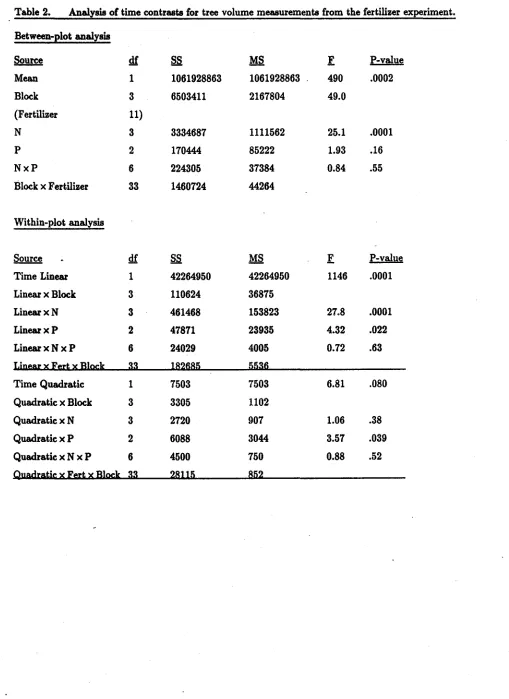
Results for the between- and within-plot analyses are presented in Table 2 for the fertilizer

example (SAS® code is in Appendix I). The fertilizer effects are partitioned into N, P and N x P

effects reflecting the factorial treatment structure. The between-plot analysis indicates that,

averaged over 2, 4, and 6 years post-application thereisa strong main effect of N on tree volume. Trends over the 6 year period are examined in the within-plot analysis. As there are three

equally spaced measurement times, values of the lin~contrast are obtained on each plot as

zi,l

=

~

(Yi;1 - Yi;3)' where the multiplier

~

simply ensures that sums of squares for the linear and quadratic contrasts will represent a partitioning of the overall sum of squares for time. The

quadratic contrast isZij2

=

~

(Yi;1 - 2Yi;!

+

Yi;9). Results for the analysis of variance of theZijl

of tree volume on time. The analysis of variance of the quadratic contrast values,Zij2' indicates whether the response over time is curved rather than linear, and whether this nonlinear component is affected by the fertilizer treatment.

Each fixed effect is tested against its interaction with blocks so that conclusions will not be c.onfined to the blocks in this particular experiment. The proper error term for testing fertilizer differences is based on the variability in fertilizer effects among blocks. Similarly, the proper error terms for testing the time contrasts are based on the variability in those contrasts from block to block, i.e. the contrast x block interaCtion. Interpretation of these F tests is discussed following the results of the MANOVA tests.

Testing hypotheses: multivariate analysis

The analysis of contrasts can be viewed as a univariate analysis in which contrasts among times areused to partition sums of squares for time and time x fertilizer effects, and the

corresponding error terms, in order to construct valid F tests. Alternatively the analysis of contrasts can be viewed as a partof a multivariate repeated measures analysis. The multivariate tests for the fertilizer effects (averaged over time) are the same as the tests in the between-plot part of the analysis of contrasts (Table 2). In addition, the single degree of freedom time contrasts are combined into composite multivariate tests for the time main effect and time x fertilizer interactions. These multivariate tests for the time main effect and the time x fertilizer interactions jQintly examine hypotheses relating to all of the p-l contrasts on time. In the fertilizer example,

the test for the time main effect puts the linear and quadratic time effects together into one hypothesis.

p+T_{1 p+T2 p+Ts} mean

P1

+ ({3T)u

P1

+ ({3T)12

P1

+ (f3Ths block 1

-:.

'\.

_B=

_P

4 + ({3T)41

P

4 + ({3T)42

P

4+ ({3T)43 block 4

....

F1 + (FT)1,1 F1 + (FT)1,2 F1 + (FT)1,3 fertilizer1

F12 + (FTh2, 1 F12 + (FTh2, 2 F12 + (FT)12,S fertilizer 12

The hypotheses are then all written in the form Ho: L B M

=

0, where the matrix L specifies the

~r'ItJ#IftJ ~

linear combinations of the between-plot factors and the matrix M specifies the linear combinations

_....

of the within-plot factors to be tested. Let

k

n contain coefficients for comparing nitrogen levels,

k

p contain coefficients for comparing phosphorus levels,

k

npcontain coefficients for

nitrogen x phosphorus interaction, and

M,

contain time contrast coefficients. In addition, let

M

0 contain coefficients to compute the mean of all times and

k

0 coefficients to compute the mean over all plots (for examples of

k

and

M

matrices see Appendix IT). These contrast matrices are put together to test the repeated measures hypotheses as follows :

Nitrogen main effect _H:

_kJ!Mo=J!,

Compare N levels averaged over all levels of P and time

Phosphorus main effect H:

k

p

l!

M

0

=J!,

Compare P levels averaged over all levels of N and time

N x P interaction Time main effect Time x Nitrogen Time x Phosphorus TimexNxP

N x P interaction averaged over all times Compalle times averaged over fertilizer levels Time x N interaction (averaged over levels of P) Time x P interaction (averaged over levels o~N) Time x N x P interaction

program that is specifically intended for repeated measures analysis). In a repeated measures analysisth~tests for fertilizer effects compare levels of Nand/or P averaged over all times, whereas in a general MANOVA the tests for fertilizer effects compare fertilizer levels for all times

simultaneously. The test for the time main effect uses the contrasts of time, Zijl andZij2'jointly, to test that the mean response over all pl,?ts is the same at each time. Any pair of linearly independent contrasts over time would result in the same multivariate tests for time main effect and interactions as the linear and quadratic contrasts presented here.

Inthe univariate analysis of variance for a randomized block design, hypotheses are tested by comparing the treatment mean squares with MSBlock x Treatment, which estimates the residual variance or error. Inthe repeated measures setting we havep x p matrices of treatment and error

mean squares. The multivariate tests are based upon these matrices of sums of squares and cross products, which play the same role as the sums of squares in a univariate analysis. For the randomized complete block design with one "between-plot" factor, A, let SSB xA

lIkbe the

block x A sum of squares for the k,h time. SSB xA

YIeis based on the residuals 'ijle=Yijle -

Y

i.1e

- Y.jle

+

Y ..Ie' The sum of products between the'residuals at the k,h and k""htimes is denoted

4 12

SPB x A....

=

E E

'i,·Ie'..

Ie"" These sums of squares and cross products are arranged in the

"1e"1e* i

=

Ij

=

1

I'

matrix

SSBxA

lI1

SPBXA

1I2111

SPBXA

1I3111,

SPBXA

lI1112

SSBxA 1I2 SPB xA

Y3112

Sum of squares and crOss product matrices are constructed for each of the terms in the model [2] in a similar fashion. For the randomized block design with one between-plot factor there are four such matrices (Table 3).

The within-plot covariance matrix, ~E , is estimated by the Block x A SSCP matrix divided

block and within-plot covariance matrices, a'~ ~

+

~ ~ This is a direct generalization of expected mean squares in the univariate analysis of variance with random block effects, and the univariate expected mean squares can beusedas a guide to determine the proper error matrix for a particular test.

The multivariate tests can be constructed directly from the matrices in Table 3 (see e.g. Johnson et. al. 1983). However, the relationship between the analysis of contrasts and the multivariate tests is more readily seen if we use thep-1 contrast variables, Zijll €=1, ...p-1, and the normalized mean, ZijO

=

~

Ie

~

lYijlel rather than the original variables, Yijl""Yijp' to

construct the matrices of sums of squares and products. Notice that the contrast variables can be formed by post-multiplying

1.,

by a contrast matrix M: ZijO

=

1.,

iiM0 and [Zijl Zij2]

=

1.,

iiMt·

The tests for between-plot effects are based on the sums of squares of ZijO' The multivariate tests of time main effects and interactions arebasedon the sums of squares of the p - 1contrasts, Zijlt Zij2' ... , Zijp-1'defined in the matrix Mto Inthe fertilizer experiment Zijl is the linear contrast, and Zij2 is the quadratic contrast. For the

,.tI.

contrast denote the

sum

of squares for a particular effect SSEffect.dl and denote the sum of cross products between the first and second contrasts SPEffect.dz2' These sums of squares and cross products are arranged in the matrix

The test for the time main effect compares the determinant of SS,9P(Mean)z' which contains sums of squares and cross products of the grand meansZ ..1and

z ..

2 of the linear and quadratic time contrast variables, with the determinant of SS,9P(Block)zl which contains sums of squares for block-to-block variation. The determinant, whic,Qisalso called the generalized variance, summarizes the information about the variances of both the linear contrast and the quadratic contrast and their covariance. The likelihood ratio test statistic is Wilks' lambda,

A _ ISS,gP(Block);c1

The hypothesis of no time main effect is rejected if A is small; i.e., if the block-to-block variation intime effects is small relative to mean differences in tree volume among times.

In general, Wilks' lambda compares an error matrix

C!)

to a hypothesis matrix

O! ),

which indicates which of the "between-plot" factors are being tested. In a univariate analysis of variance for a randomized block design, the fIXed treatment factors are tested against the mean square,for interaction with blocks. Similarly, in the repeated measures case, the error matrix for testing a "between-plot" factor is the block x "between-plot" factor SSCP matrix. The general form of

_....

Wilks' lambda is

For the hypothesis that the time main effect equals zero, !!=SS,gP(Mean)~and! =

SS,gP(Blockl.. The matrices for testing fertilizer x time interactions are !! = Ss,gP(Fertilizer)~and ! = SS,9P(Block x Fertilizer).. The fertilizer main effects could also be tested using a Wilks' lambda statistic with

J!

=

SS,9P(Fertilizer)--o and !

=

SS,9P(Block xFertilizer)~o' but since only one variable,

Zo,

is involved, the matrices! and!! are scalars ( each involving only a single sum of squares) and the test statistic reduces to the usual F statistic,

MSFertilizer% /MSBlock x Fertilizer% • The distribution of Wilks' lambda depends on the

o

,

0

hypothesis degrees of freedom, d_{h ,} the error degrees of freedom, de' and on the number of contrasts for the within-plot factor, c=p-1. The test can only be carried out if d_e+l

>

Co In a randomized complete block design with time as the repeated factor, the number of blocks must exceed the number of time contrasts. Critical values for hypothesis tests are given in Appendix III.

Time main effect;

[

42264950 563133 ]

ss.gp(meaa).=' 563133 7503

A=.002135, p-l=2, d_h=1, d_e=3 test statistic=467.3, p=.002

FertilizerXTime interactions;

[

182685 SSCP(BlockxFertilizer)..

= .

- 5819 5819 ] 28115 [ 110624 SSCP(block)"

=

- 9353 9353 ] 3305 [ 461468 SSCP N

-- ( ).. - -6101

d_h=3, A=.2569

test statistic=1O.38 p:.0001

-6101 ]

-f

47871

2720 ss.gp(P)..

~

14453

d_h=2, A=.6826

test statistic=3.366 p:.015 14453 ] 6088

1

24029 SSCP(NxP).. - 8499

d_h=6, A=.7805 test statistic=.7034

p=.74

8499 ] 4500

The linear and quadratic effects of time (averaged over fertilizer levels) from Table 2 are tested simultaneously by the Wilks' A test for time main effects. There are significant changes in tree volume over time (Wilks' lambda for time main effect, p:.002), and the interaction tests indicate that the change over time depends on both the N and P fertilization rates (Wilks' lambda, p=.OOOl for N x time interaction and p=.015 for P x time interaction). From the analysis of contrasts in Table 2 we see that the rate of increase of tree volume depends on N (F-test for N x time linear effect, p=.OOOl). Italsoappears that the increase in volume with time is not linear and the amount of curvature depends on the level of P (F-test for P x time quadratic effect, p=.039). In the original analysis (Vose and Allen 1988), increase in volume from the time of fertilizer application was analyzed rather than volume itself. The multivariate tests for time and

standard error ofz ..Ieis s(z ..k)

=

(Valentine and Allen 1990) the authors have used volume at the time of fertilization as a covariate. Volumeattime zero can be incorporated into the repeated measures analysis as a "between-plot" covariate. Inthis particular data set inclusion of the covariate has the effect of substantially decreasing both the unexplained variation among blocks and the residual error and of drawing out a significant Pmain effect. We omit the covariate here simply to demonstrate the repeated measures method of analysis. Inthis data set the variance increases with time, which usually is an indicationthat~a log transformation should beusedto stabilize the variances; however in the repeated meaSures analysis there is no requirement that variances be constant across time, so the analysis can be performed in the original scale, making interpretation and presentation of results simpler.

Estimation of contrasts or polynomial coefficients

In addition to testing hypotheses, estimation of the treatment means of the variables ZijO' ..., Zijp -1is also important (see also Meredith and Stehman 1991). In our example the z· variables are orthogonal polynomial contrast variables, so the mean ofZij1 for the

lh

fertilizer treatment(Z.j1)gives the linear effect for the

lh

fertilizer level, while the mean for Zij2(Z.j2)

gives the estimated quadratic effect. The fact that blocks are considered to be random replication must be takell into account when obtaining the standard errors of the estimated linear and quadratic effects. The standard error for the linear term for the

lh

fertilizer level is computed from a weighted average of two mean squares, MS;

=

4

(MSBlock_z

+

(t-l) MSBxFz ), where t

1 ~ 1 1

W

s

*

is the number of fertilizer treatments. The standard error is s(z.jl)

=

~,where

n.jis the

.J

number of plots receiving the

lh

fertilizer treatment. The mean values ofZijO' Zijl' andZij2for the mean of all blocks and all fertilizer treatments, z ..0'z ..1'and z ..2' respectively, provide estimates of the mean, linear, and quadratic effects of time averaged over all fertilizer levels. The

MS Block"

experiment. The estimated mean, linear, and quadratic effects for each nitrogen and phosphorus level, along with their standard errors are given in Table 4.

The intercept and slope in the quadratic regression equation relating tree volume and time both increased as N increased. The effect of phosphorus on intercept and slope was not linear. Mean tree volume and the rate of increase oNree volume were greatest at 28 kg P jha. The fitted curve for the treatment corresponding to the highest level of N and the middle level of P (the 11th fertilizer level), which gave the maximum response was:

Y.11k

= 5099 • Zo + 1091 • z1 + 13.19 •

z2·

(223.1) (36.67) (to.57)

Standard errors of the regression coefficients are in parentheses. Since there were no significant N x P interactions, each of the coefficients was obtained by adding together the grand mean, the N=336 effect, and the P=28 effect from Table 3; for example, the first term is. 5099=4703.56 + (5014.86444-4703.56) + (4787.82144 - 4703.56). The standard error is the square root of

Var(z~11k)

=

l<O'~

..

k+~

..

1c)'which is estimated by 1s<MSBlock.._1c+5. MSB x F.-111). In general, for a randomized block design with

r

blocks and two between-plot· treatment factors, A with a levels and B with blevels, and· no significant A x B interaction, the variance of a fitted value is

t

0'~

..1c+

a+r~b

1

0'~%1c

(for details see Appendix IV). In terms of years from fertilizer

application, the model for predicting tree volume is

not be computationally feasible to fit an ordinary polynomial. Insuch a case orthogonal polynomials must beused.

The procedure of computing separate regression coefficients for each plot which are then subjected to further analysis produces efficient estimates of the coefficients if there are a total ofp

independent z Variables; i.e., if.the model for the repeated factor is saturated. For the case of a polynomial of order less than p-1, no single estimator is most efficient and several different

estimaton have been proposed (Timm 1980). The procedure just described has the advantage that its exact distribution is known, so that the significance levels of hypothesis tests are exact, the parameter estimates are unbiased, and the standard erron given above are exact. Ithas the additional advantage that the procedure is relatively simple to implement.

Split plot design with repeated measures Experimental situation

Here we consider the standard split plot design withmainplots

in

complete blocks. Levels of the main plot factor A are assigned randomly to main plots within blocks, and levels of the subplot factor B are assigned randomly to subplots within each main plot, (i.e., there is no "stripping" of levels of either A or B). In every subplot, measurements are taken at each of p times (or at each ofplocations). In contrast to the levels of facton A and B, levels of the repeated measures factor, time or location, are not allocated randomly.

Family (Fam), with 3levels, was the subplot factor B, and within each chamber each family was assigned randomly to one of3sectors. There were5plants per family in each sector or subplot (300 plants inall). Measurements of various aspects of growth were taken on each plant on 12 occasions during the second year after plots were established. For illustration, we will analyze the increase in total height (relative to height before 03exposures began) determined on 6pccasions about a month apart and averaged over the 5 plants in a subplot. Thus for each subplot there are

6growth measurements, and the repeated measures factorisdate, with levels corresponding to 29,

57,85, 113, 156and 183 days after 3.25.87. For space reasons, the complete data setisnot presented.

Assumptions and model

We assume that the main and subplot factors represent fiXed effects, but block effects are random. Time main effects are fiXed but timexblock interaction effects are of course random. Again the systematic nature of the repeated measures factor, time, makes it necessary to allow for possibly different conelations between measurements over time within the same subplot.

Similarly, the "equal correlations" assumption may be incorrect for observations across time within the samemainplot, or within the same block. Measurements in different blocks are uncorrelated. The resulting model is presented in detail for completeness, but the detail could be skipped at first reading.

Without using vector notation, the linear modelis

[3] _{Y iiil}

=

p+ ,8i+Ai+£ii+Bi + (AB)ii+0iii_{+Te + (,IIT)ie +} (TA)ie +(JiiI.+ (TB) it + (TAB)iiI.+ 1'iiie

TheAi' _{Bi and (AB)ii are fiXed main'and interaction effects for the factors A and B; and Te,} (TA).1.' (TB)il. and (TAB) ·il. are a fiXed time (or location) main effect and corresponding fiXed

J J .

Var(Eij)

=

6:

and Vare6ij

,J

=

6:.

The (PT)ie' (Jije' and 'Yijlte' represent random time-specific contributions for blocks, mainplots, and sub plots, respectively, with

{

Oifi¥:f

Cov«PT),II,

(,BT) ..

11*)

=

'.

if' _

'*

K , f. 6

{JTee* .

I - I

{

o

ifij

¥:

f r

Cov(8 ..• , 8 ...*)=

'*'* ,

'If. , 1 f. 6

oee

*

if ij

=

IJ and

{

o

if ijk

¥:

frk*

COV('Y"LII, 'Y .... L*II*) =_{'1"'f. , 1 I< f. 6}

_'"fee*

if .... - '*'*k* •_{IJIl - IJ}

Now let Yijlt represent the row vector ofprepeated measurements for the ijk

th

subplot.' For example, lijlt = (Yijltl' Y ijltJl "', Yijlt8) for a plant in the ozone study. The more compact vector representation of the model in [3] is then

[4]

Y'J'L=_{_, '" !:}

u+p.+

_{_, 91}A.+€ .. +BL+(AB)'L+6"L_{-'I -I< - -'I< -VI<}

where each of the vectors haspelements, corresponding to each of the pmeasurement times, and Var(lijV =

l;{J

+ l;c+

l;s

Cov(liji' lijlt*) =

l;{J

+l;(

Cov(lijlt' li,'*It*) =

l;{J

for observations in the same sub-plot, for different sub-plots in the same main plot, for different main plots in the same block, Cov(Y,:,;It' Y.... L*) = 0 for plots in different blocks.

-~ -"I<

-The covariance structure for the model in [4] is related to that in [3] as follows: the

ee*th

element (relating tomeasurements at times

e

and

e*)

of

I:{J

is

6:

+

6

({JT)tl* ,

element

ee*

of

I:

_cis

6:

+

6

_oee*'

and element U* of

I:6

is

6:

+

iT

'"f

et

*.

Although variances and covariances are allowed

Analysis: hypothesis and test procedures

Except for the need to earry out additional tests for effects involving the subplot factor, the analysis for the split plot design with repeated measures is analogous to that described for the randomized complete block design. We therefore omit most of the detail and illustrate the main features of the analysis using the Os - acid rain study as an example.

Again it is useful to think of the analysis as consisting of two parts, a between-plot analysis and a within-plot analysis. The between-plot analysis is a split plot analysis applied to the subplot means computed by averaging over all 6 levels of the repeated measures factor, date. In the between-plot analysis, MANOVA and the "analysis of contrasts" yield identical tests, and all tests

rel~teto effects of the main plot and subplot factors averaged over dates. The within-plot analysis provides tests for all effects involving the repeated measures factor, date. Omnibus multivariate tests are carried out, as well as tests aimed a~more specific aspects of the repeated measures factor. These latter tests are usuallybasedon using orthogonal contrasts to partition the effect of the repeated measures factor, resulting in a series of p -1separate split plot analyses, each on a different contrast. Interpretation of the omnibus multivariate tests and the contrast - based tests· is given below.

Plotting growth against date for the various Os-acid rain treatments (Fig. 1) suggested that a simple polynomial equation would describe the response curve, and so orthogonal polynomial contrasts wereusedto partition the date effect. Results for the between-plot analysis (on the means over dates) and sums of squares for thep-1

=

5 polynomial contrasts are presented in Table 5. Note that for simplicity the factorial structure of the main plot treatments has been suppressed, the main plot factor being denoted "Trt", the subplot factor being "Fam".

All tests in the between-plot analysis relate to effects that are averaged over dates. Thus the test for Trt tests the null hypothesis that mean growth (averaging over the 6 dates and over the 3 families) is the same for each of the 10 OsXpH combinations. In the notation of model [3],

combination. Similarly, the test for Fam is a test for no family main effect averaging both over the

10

Trtsand over the 6 dates. Inthe notation of

[3],

_{the null hypothesis is Ho: B1}

=

B₂

=

_B3, where B_i is the main effect for the

f-h

family. Only the Fam main effect appears important, but before concluding that Trt effects are nonsignificant it is necessary to examine results for the interactions with date in the within-plot part of the analysis.

Inthe within-plot analysis, the MANOVA test for a date main effect would .test that mean height (averaging over treatments and families) is the same at each date. Altematively, this test can be interpreted as testing simultaneously that the linear, quadratic, up through quintic,

components of the regression of height on date are each zero. The analysis of contrasts differs from MANOVA in that a separate test is performed for each of the polynomial contrasts. In the 03-acid rain example, the MANOVA test for date cannot be carried out as there are only two blocks, yet the main effect for each ofth~five polynomial contrasts can be tested separately via the analysis of contrasts. Insituations like this where the number of blocks is less than the number of

measurement times, we suggest limiting attention to two or three contrasts (selected a priori) as a compromise between not performing a test for a date main effect and on the other hand possibly incurring an unsatisfactory type I error rate because of multiple testing (see also Eskridge and Stevens 1987).

consistent with our recommendationto limit attention to only a few contrasts when the number of blocksisleu than the number of levels of the repeated measures factor.

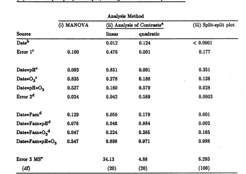
Results for the tests carried out in the within-plot analysis are presented in Table 6 for the linear and quadratic contrasts. The p-values for the omnibus MANOVA tests (excepting, of course, the test for a date main effect) are also given in Table 6. Note that the factorial structure of the main plot treatments is recognized in Table 6 and the effects for Trt partitioned into pH, 03'and pH x03components. Alsoindicated in Table 6 are the error terms for each of the F tests iI:l the analysis of each contrast, and the analogous error matrix usedin the corresponding MANOVA test. As noted above, F tests for each contrast are conducted as for a split plot design with main plots in blocks, blocks assumed random, and with a test for the grand mean being zero included.

The MANOVA tests suggest that there are no strong interactions between date and any of the main or subplot factors, i.e., that the growth curves are similar across treatments.. If a 10% significance level isusedthen there are indications of possible differences in growth among the combinations of pH, 03'and Fam(p=.093for Date x pH,p=.076for Date x Fam, and p=.047for Date x03x Fam).

Compared to the multivariate tests, those carried out in the analysis of contrasts can have greater power for detecting treatment x time interactions if the effect of date or time can be summarized in one or two contrasts. This is analogous to the increase in power for specific hypotheses obtained by partitioning a treatment sum of squares into components representing, for example, factorial

main

and interaction effects. Results for the analysis of the linear and quadratic contrasts on date are therefore of interest, even if the MANOVA tests are largely nonsignificant.

families, the regression of growth on date has the same "slope" or linear component for the two pH

levels. Similarly, the test ofDat~Famtests the nun hypothesis that, averaging over all 10 levels

ofTrt, the regression of growth on date has the same slope for each of the 3 families. The

Date*pH*Fam interaction tests whether (averaging over Os levels) the difference between slopes for

the two pH levels is the same for each of the 3 families.

Interpretation of the tests for the quadratic contraSt is the same except that "quadratic

component" is substituted for "slope" or "linear component". There appear to be differences in

the linear components of the regressions for families and these difierences depend on pH

(p

=

.050

andp

=

.046 for the Fam and pH x Fam effects, respectively). A slightly stronger effect is that the

curvature of the regressions for the 2 pH levels seems to be different (p

=

.001 for pH in the

analysis of the quadratic contrast). Plotting mean growth for the 6 pH x Fam combinations

against date shows that growth appears to be slightly greater for rain~t pH 5.2 than for pH 3.5 in

families 2,and 3, but the opposite is true in the last two months for family 1. Asnoted in Kress, et al. (1988), data from subsequent years should help to determine whether this represents a real

,

effect of the rain acidity or not.

Neither the linear nor the quadratic contrast on date indicates a significant effect of Os

concentration on growth, although Kress et al. (1988) note that growth was suppressed at the two

highest Os levels. The Os interaction effects could be examined more closely by partitioning them

into appropriate contrasts in Table 6, but we have chosen instead to keep the analysis as simple as

possible.

Finally, we comment on an approach that is often incorrectly used. for the analysis of data

such as the Os-acid rain growth data. This approach is tocarryout a split-split-plot analysis, treating the repeated measures factor date as a sub-sub-plot factor, and results for effects involving

date from the sub-sub-plot part of this analysis are given in Table 6 for comparison with the

MANOVA and analysis of contrasts. Validity of these sub-sub-plot tests requires homogeneity of

on height, not only because of the systematic nature of the factor time or date, butalsobecause variance tendstoincrease as mean height increases. Evidence that the variance-covariance structure is not independent of date is seen in the error sums of squares (i.e. Date x Bl x Fam(Trt» for the polynomial contrasts in Table 5. These sums of squares should be of about the same magnitude under homogeneity of variances and covariances, but are seen to differ by up to 2 orders of magnitude. For repeated measqres data, dependence on time of the variance-covariance

structure will tend to result in liberal tests, that is, tests which produce too many significant outcomes (e.g. Meredith and Stehman, 1991). From Table 6, we see that the agreement between p-values produced by the split-split-plot tests and those produced by the MANOVA tests is poor, even though the hypotheses examined are equivalent. The tests

hUed

on the linear and quadratic contrasts examine more specific hypotheses and so p-values need not agree even qualitatively with those from the split-split-plot analysis or MANOVA. Generally, however, there is a tendency for the split-split-plot tests to suggest the presence of stronger treatment and family effects on growth than either the MANOVA or analysis of contrasts. Asplots do not indicate strong effects on growth (see Figure 1) this illustrates that the split-split-plot p-values can be misleading.

Discussion and condusioDS

treatments. The analysis of contrasts is more flexible than the multivariate analysis, so sometimes only part of the full analysis can be completed. For example, in randomized block designs it often happens that there are more levels of the repeated factor than there are blocks. In this case it is not possible

to

compute the multivariate test statistic for the repeated factor main effect. It is, however, still possible to test the individual contrasts of the repeated factor. Even when there are only a few levels of the repeated factor, if there are only three or four blocks the multivariate test may tend to lack power (Davidson 1972). When the number of blocks is small, the analysis of contrasts may prove more informative than the multivariate tests. Instandard software such as the SAS PROC GLM "REPEATED" statement the multivariate tests require a complete set of observations for every plot. Ifa few data points are missing from one or more plots, it is still possible to do the analysis of contrasts, using PROC GLM without the "REPEATED" statement.

There are some situations for which the methods of this paper are not adequate. If more than a few data points are missing orifthe levels of the repeated factor are different for different plots then the multivariate analysis is impossible and the analysis of contrasts may be less efficient than methods such as estimated generalized least squares. Covariates that vary from plot to plot can be incorporated into the analyses presented in this paper, but covariates that vary over time, such as rainfall between measurement times at different sites, cannot. In these circumstances more sophisticated methods such as estimated generalized least squares or restricted maximum likelihood should beusedrather than the repeated measures analysis presented here (Schaalje et al. 1991, McLean et al. 1991). Growth~urvesare usually s-shaped, with growth approaching an asymptote, and are not fit very well by polynomials. Ifthe aim is to describe and predict growth by fitting a mathematical model, then a nonlinear model with an appropriate covariance structure accounting for correlations over time should beused(Lindstrom and Bates 1990, Vonesh and Carter 1991).

way to obtain more information from a flXed amount of experimental material. When planning a repeated measures experiment, the number of blocks should exceed the number of contrasts needed to describe the effect of the repeated factor. Inorder to compute all of the multivariate test statistics at least as many blocks are required as there are levels of the repeated factor. Itis reasonable to require more experimental units in a repeated measures design because each

experimental unit provides information on a possibly complex time (or location) effect. Muller and Peterson (1984) give methods for computing the power of multivariate tests which can be used in planning sample sizes.

Some texts recommend randomizing the order of treatments on each experimental unit (e.g. Johnson and Wichern 1988). Inforestry the most commonly used repeated measures factors, such as time, depth, and distance from the row, cannot be randomly allocated. If the experimental unit is the tree and different treatments are applied to different leaves or branches of each tree, the treatments should be randomly allocated. Cases where different treatments are assigned to each experimental unit at different times are more complicated. Examples include crop rotation studies and studies involving human subjects. For instance, in a study of the eftlcacy of three different remedies for chronic pain, each patient might receive all three drugs given in random order, spaced out at suitable time intervals. In this type of design there are possible complications of order effects and carry-over effects from one time period to the next and there is the additional problem that it is difficult to know whether correlation patterns should be caused by the passage of time or by the individual's type of response to different types of treatments. That is, should the repeated factor be "drug" or should it be "time" for purposes of estimating the covariance matrices?

fIXed effect differs from the case when both factors are f1Xed in two respects:

1. The enor term for testing the main effect of the fixed factor involves the sum of squares for

the interaction of the fixed effect with the random effect. This is true for all univariate and

multivariate tests. For example, if A is fixed and B is random, then the univariate and

multivariate test statistics are F=MSA/(MSAXB), and

A=I S8,9P(AXB)~SS,9P(A)

+

S8,9P(A x B)~ respectively. The proper tests may not be

provided automatically by standard statistical software and it maybenecessary to write a

few extra commands to compute them.

2. Standard errors of treatment means and regression coefficients incorporate the variation

among levels of the random factor as well as the within-plot variation. They are not simply

computed from MSE. The proper standard errors canbedetermined from inspection of the

. univariate expected mean squares. Again, statistical software may not provide the correct

standard errors, and some hand computations mayberequired. Usually the standard errors

for treatment means averaged over levels of a random factorwillbelarger than if all factors

had. been fixed.

Acknowledgments

We thank H. Lee Allen and Lance Kress for providing the air pollution data set, and the North Carolina State Forest Nutrition Cooperative and Weyerhaeuser Company for use of the

M.L. Gumpertz~29 References

DAVIDSON, M.L. 1972. Univariate versus multivariate tests in repeated-measures experiments. Psychol. Bull. 71: 446-452.

ESKRIDGE, K.M., and STEVENS, E.J. 1987. Growth curve analysis of temperature-dependent phenology models. Agron. J. 79: 291-297.

JOHNSON, D.E., CHAUDHURI, U.N., and KANEMASU, E.T. 1983. Statistical analysis of line-source sprinkler experiments and other nonrandomized experiments using multivariate methods. Soil Sci. Soc. Am. J. 47: 309-312.

JOHNSON, R.A., and WICHERN, D.W. 1988. Applied Multivariate Statistical Analysis, Second

Ed. Prentice Hall, Englewood Cliffs, NJ. 607 pp.

KEMPTHORNE, O. 1952. The Design and Analysis of Experiments. Reprinted 1979. Robert E. Krieger Publishing Co. Huntington, NY. 631pp.

KRESS, L.W., ALLEN, H.L., MUDANO, J.E., and HECK, W.W. 1988. Response of loblolly pine to acidic precipitation and ozone. Proceedings of APCA 8lat Ann. Mtg. Dallas, TX. LINDSTROM, M. J., and BATES, D. M. 1990. Nonlinear mixed effects models for repeated

measures data. Biometrics. 46: 673-687.

MCLEAN, R.A., SANDERS, W.L., and STROUP, W.W. 1991. A unified approach to mixed linear models. Am. Stat. 45: 54-64.

MEREDITH, M.P., and STEHMAN, S.V. 1991. Repeated measures experiments in forestry: focus on analysis ofresponse curves. Can. J. For. Res. 21: 957-965.

MORRISON, D.F. 1990. Multivariate Statistical Methods, Third Ed. McGraw-Hill. New York. 495pp.

MOSER, E. B. , SAXTON, A.M., and PEZESHKI, S.R. 1990. Repeated measures analysis of variance: application to tree research. Can. J. For.ReS. 20: 524-535.

ROWELL, J.G., and WALTERS, D.E. 1976. Analysing data with repeated observations on each experimental unit. J. Agric. Sci. 87: 423-432.

SCHAALJE, B., ZHANG, J., PANTULA, S.G., and POLLOCK, K.B. 1991. Analysis of repeated-measurements data from randomized block experiments. Biometrics 47: 813-824.

TIMM, N.H. 1980. Multivariate analysis of variance of repeated measurements. Handbook of Statistics, Vol. I, P.R. Krishnaiah, ed. North-Holland Publishing Co. pp 41-87.

VALENTINE, D.W., and ALLEN, B.L. 1990. Foliar responses to fertilization identify nutrient limitation in loblolly pine. Can.J. For. Res. 20: 144-151.

VONESH, E.F., and CARTER, R.L. 1991. Mixed effects nonlinear regression of unbalanced repeated measures. Biometrics. In press.

M.L. Gumpertz - 31

Table 1.

Tree volume (fts/acre) from loblolly pine mid-rotation fertilization experiment.

Block 1

Block 2

Block 3

Block 4

N P

Year

Year

Year

Year

(kg/ha) (kg/ha)

2

4

6

2

4

6

2

4

6

2

4

6

0

1658 2119 2687

1755 2272 2762

2068 2618 3208

2237 2921

3623

0

28

1726 2249 2843

1847 2376 2909

1988 2511 3133 2115

2784 3412

56

1794 2375 3007

1839 2332 2914

2006 2608 3250 2247

2742 3398

0

1788 2329 2742

1864 2387 2988

2159 2840 3418 2387

3051 3765

112

28

1989 2575 3242

1976 2615 3250

2160 2837 3532 2106

2698 3318

56

1805 2424 3024

1850 2447 3053

1999 2618 3192

2181

2777 3498

0

1875 2502

3054

1913 2556 3169

2149 2893 3685

2409

3155 3847

224

28

1812 2412 3089

1981 2659 3432

2293 3063 3855

2490

3273 4091

56

1819 2497 3208

2089 2769 3703

2263 3076 3873

2283

2826 3535

0

1934 2675 3313

1984 2637 3339

2381 3093 3843

2336

3068 3764

336

28

2116

2926 3681

1964 2713 3472

2237 2968 3832

2523

3328 4276

Table 2. Analysis of time contrasts for tree volume measurements from the fertilizer experiment. Between-plot analysis

Source df _~ MS

_F.

P-value

Mean

1 1061928863 1061928863 490 .0002

Block 3 6503411 2167804 49.0

(Fertilizer 11)

N 3 3334687 1111562 25.1 .0001

P 2 170444 85222 1.93 .16

NxP 6 224305 37384 0.84 .55

Block x Fertilizer 33 1460724 44264

Within-plot analysis

Source df _~ MS

_F.

P-value

Time Linear 1 42264950 42264950 1146 .0001

Linear x Block 3 110624 36875

LinearxN 3 461468 153823 27.8 .0001

LinearxP 2 47871 23935 4.32 .022

LinearxNxP 6 24029 4005 0.72 .63

Linear x Fett x Block 33 182685 5536

Time Quadratic 1 7503 7503 6.81 .080

Quadratic x Block 3 3305 1102

Quadratic x N 3 2720 907 1.06 .38

Quadratic x P 2 6088 3044 3.57 .039

Quadratic x N x P 6 4500 750 0.88 .52

Table3. Matrices ofsumsof squares and cross products for a randomized complete block design

Source

Mean

Block A

BlockxA

1

b-l

.1

(b-l)(.I)

matrix

ss,gp(Mean}y

ss,gp(Block)y

SS,9P(A}y

SS,gP(Block x A}y

t

Degrees of freedom associated with each element of the matrix. Number of blocks=b, levelsof

Table4. Mean, linear, andquadratic time effects for levels ofN and P in the fertilizer example.

N(kgJha)

.fa

o

4346

112 4565

224 4888

3361 5015

817.1

869.6 1011 1055

20.82 3.062 18.88 7.246

P(kg/ha)

Zo

o

4663

28 4788

56 4660

std. efrort 216.8

897.6

974.5

943.0

31.60

-3.266 18.45 22.33

7.645

std.

mot·

218,9 33,38 8.729

~MSBIOCk.ll

+

3· MSB x

F.II

*

S.E.

=

'4.12

k.

Table 5. Between plot analysis and within plot sums of squares for the pine seedling growth (cm)

datameasured on 6 dates in the ozone-acid rain study.

Between-plot analysis

Source df SS F P-value

Block 1 38.94 0.16 0.700

Trt 9 2805.13 1.26 0.367

Block.Trt& 9 2219.51 1.91 0.109

Fam 2 1186.78 4.60 0.023

Trt.Fam 18 2092.32 0.90 0.586

BlocbFam(Trt)b. 20 2582.34

Within-plot analysis - sums of squares for the 5 orthogonal polynomial contrasts on date

Date Date Date Date Date

Source df linear quadratic cubic quartic quintic

Date 1 138293.8 2370.4 335.45 5.64 2.15

Date.Block 1 47.2 92.4 0.74 9.98 2.25

Date.Trt 9 1242.3 130.9 11.28 37.34 4.04

Date.BlocbTrt 9 767.6 36.9 34.19 7.36 7.82

Date.Fam 2 239.1 18.3 5.23 0.33 0.89

Date.Trt.Fam 18 699.6 55.6 27.71 24.84 16.17

Date.BlocbFam(Trt) 20 682.7 97.7 20.62 20.74 7.59

Table 6. Within-plot analysis of growth data from the ozone-acid rain study. P - values for tests of Date effects based on (i) MANOVA, (ii) analysis of orthogonal polynomial contrasts on Date, and (iii)an invalid split-split-plot analysis, treating date as a 8U~8U~plotfactor.

Analysis Method.

(i) MANOVA (ii) Analysis of Contrasts& (iii) Split-split plot

Source linear quadratic

Dateb 0.012 0.124

<

0.0001

Error 1c 0.100 0.476 0.001 0.177

Date*pBc 0.093 0.851 0.001 0.351

Date*Osc 0.835 0.278 0.188 0.136

Date*pB*Os 0.537 0.160 0.579 0.028

Error ~ 0.024 0.042 0.589 0.0003

Date*Famd 0.129 0.050 0.179 0.001

Date*Fam*pBd 0.076 0.046 0.884 0.002

Date.Fam.Osd 0.047 0.324 0.385 0.165

Dare.Fam*pB.Os 0.547 0.898 0.971 0.998

Error 3 MSe 34.13 4.88 8.293

(dt) (20) (20) (100)

&Polynomial contrasts of degree greater than 2 accounted for only a small fraction of the variation blndicates effect tested against Error 1 (Date*Block Error)

CXndicates effect tested against Error 2 (Date.Main plot Error) dlndicates effect tested against Error 3 (Date*Sub plot Error) eFor univariate analyses only

•

FigureLegend

Figure 1. Mean growth (increase in height from 3.25.87) measured at 6 dates after 3.25.87 for 3 families of loblolly pineexposedto "rain" at pH 5.2 or at pH 3.5. Shaded symbols (0,0,and b.) represent means for families 1,2, and 3 respectively, for rain at pH 3.5, and open symbols (0,0,

Figure 1.

O.

I'-o

<0

•

•

0

g,

i

•

••

o

'(W)

a

i

o

C\I

~

_o

•

•

o

~

~_.----..--_--.-

...I

,...

. .

.

29

85

156

•

M.L. Gumpertz - 39

Appendix I. SAS commands for randomized blocks with repeated measures

The SAS statements for producing the multivariate tests and the analysis of polynomial

contrasts are given below. The "REPEATED" statement provides tests for N, P, and time main

effects and their interactions, but uses the residual error matrix, SSCP(Block x F), for all tests.

This is appropriate for tests involving thebetween~plotfactors N and P, but not for the time main

effect. The "MANOVA" statement is included to compute the tests for the time effects using

SSCP(Block) as the error matrix. The "SUMMARY" option on the "RE~EATED" and

"MANOVA" statements provides the analysis of variance tables for the linear and quadratic

contrasts.

PROC GLM DATA=LOBLOLLYj

CLASS BLOCK N Pj

MODEL Y1 Y2 Y3 = BLOCK N P N*P / NOUNIj

REPEATED TIME 3 POLYNOMIAL / PRINTH PRINTE SUMMARYj

MANOVA H=INTERCEPT E=BLOCK M=(111) MNAMES=MO/ ORTH SUMMARYj

MANOVA H=INTERCEPT E=BLOCK M=(-1 0 1, 1-2 1) MNAMES=LINEAR QUAD /

PRINTH PRINTE SUMMARY ORTHj

The next set of SAS statements produces the estimated values of the contrasts. The

"LSMEANS" statement produces means of the regression coefficients for different levels of N and

P. The fitted value for a particular fertilizer level (assuming there is no N x P interaction) can be

obtained using the "ESTIMATE" statement as in the example (N=336, P=28), but the standard

error must be computed by hand. The standard error printed out by the "ESTIMATE" statement

DATA Z;

SET LOBLOLLY;

ZO=(Y1+Y2+Y3)/SQRT(3); Z1=(Y3-Y1)/SQRT(2);

Z2=(Y1- 2.Y2

+

Y3)/SQRT(6); PRoe GLM DATA=Z;

CLASS BLOCK N P;

MODEL ZO Z1 Z2 = BLOCK N P N.P ; LSMEANS N P;

M.L. Gumpertz - 41

AppendixU.

k

and

M

matrices for the fertilizer experiment.

Factor

Mean

(across

plots)

Nitrogen

Phosphorus

NxP

Mean (across times)

Time

Contrast Matrix

k

0

=

s:ta

[12 3 3 3 3 1 1 1 1 1 1 1 1 1 1 1 1]

[

0 0 0 0 0 1 1 1 0 0 0 0 0 0 -1 -1 -1]

k

n=~

.

0 0 0 0 0 0 0 0 1 1 1 0 0 0 -1 -1 -1

"40 0 0 0 0 0 0 0 0 0 0 0 1 1 1 -1 -1 -1

1 [0 0 0 0 0 1 0 -1 1 0 -1 1 0 -1 1 0 -1]

k

p

=

rs

0 0 0 0 0 0 1 -1 0 1 -1 0 1 -1 0 1 -1

o

0 0 0 0 1 0 -1 0 0 0 0 0 0 -1 0 1

o

0 0 0 0 0 0 0 1 0 -1 0 0 0 -1 0 1 . 1 0 0 0 0 0 0 0 0 0 0 0 1 0 -1 -1 0 1

k

np

=

2'

0 0 0 0 0 0 1 -1 0 0 0 0 0 0 0 -1 1

o

0 0 0 0 0 0 0 0 1 -1 0 0 0 0 -1 1

o

0 0 0 0 0 0 0 0 0 0 0 1 -1 0 -1 1

MO=~U

]

[

_1/..J2

.1/~

]

M,=

0 -2/~

1/..J2 1/~

Any set of p-1linearly independent contrasts of the repeated factor could be used in the

M

t

matrix since the multivariate tests for time main effect and time x fertilizer interactions are

invariant to the particular choice ofcontras~s. All contrasts in the

M

matrices have been scaled so

Appendix

m.

Test Statistics and Critical Values for Wilks' Lambda

Reject Boifthe test statistic exceeds the critical value (Morrison 1990).

Case

min(d_{h ,} c)=l

min(d_h, c)=2

Test Statistic Critical Value

ifde is large

Symbolsinthe table:

c

=

p - 1, the number of contrasts of the within-plot factor

d_h

=

hypothesis degrees of freedom (For a factor, A, with a levels, d_h

=

a-I)

•

•

to

AppendixIV. Fitted values and standard errors of coefficients

Fora randomized block design with two treatment factors, F and G, we first fit a treatment means model,z'i= P

+

fJ,

+

Ai

+

f'i' whereAiindicates the

j'''

treatment combination (which is a combination of factors F and G). If there is no significant FxG interaction then the fitted

coefficients,

i.i'

for the

j'h

treatment are estimated using an additive model and switching to double subscripts to denote the levels ofF and G (where i=1,ou,b blocks, £=1,...,f levels ofF,

m=1,...,g .levels of G) gives

=z

_•••

+f";

_{\6 •.,.}1/

-z

_•••)+tz_{\4 .•m}

-z)

_..•

_1+g-1

f

Z. +1- 1

f E z .

1 +9- 1

f -

E z",

big ,

=

1

.em

Tfii,

=

1

m'

~m .£m bIg,

=

1

e'

~£if.m

1 b

-rp

E

E

E

Z.", I'

OTg i

=

1 £1~£ m'~ m If.m

Writing eachz'iin terms of the model elements yields the variance expression, Var(

i .) -

J.a2

+1+9-10'2

. , - 0-fJ big ('

The variance of any linear combination of coefficients can be found by working with the matrix formulation of the repeated measures model,

[

Y

11]

7

= -,

=

X

fJ

+. ,

where there are b blocks and • trealmentB.

# v . . . ....

'Z"

To describe the effect of the repeated factor using a polynomial model, express

_{.... .... ....}

fJ

as"I M', where

•

2,.

2WoCil

1 1 1

T = and M'= t₁ t₂ t₃

#'V #'V

2

".,1

t₁2 t2₂ t2₃

2

".,12

The elements of 7 are the regression coefficients (for the regression on time) for the treatment

#'V

groups defined in the! matrix. The row veetors Z e/feeteach contain an intercept, a slope, and a quadratic coefficient; e.g., Z" =

h

,,1"'1,,2"'1~. Our interest lies in estimating

2

and linear

combinations of the elements of T •

#'V

Incorporating the model for the time effects into the repeated measures model gives:

vec<z. ') = (! 0

M)

vec(Z ')

+

vec({, ').

Vec(t ') =

tt

u·"!

t>J'

contains the observation vectors for all n..=ba of the plots stacked on top of each other. Vee (T ') = [T .. T_{, . " , . " ,., ff'W}blockl ..._{, . "}Tbloekb_{, . "}Ttmtl ...T _tmtJ' contains all of the

fIlftI

parameters for the regression of the response variable on time. The ordinary least squares estimator for vee(T ')is

rv

vee(:; ') = [(X'X)-IX '0 (M/M)-IM1 vec(y ').

#IV ,..", fIIW #"tt# fIIW,." , . " .,.""

For the repeated measures model with a treatments arranged in b randomized blocks, the

covariance matrix of vee(y ') is block diagonal, rv

Var(vee<.t

'»

=

[Q.

0 ! ! ') 01JJJ1

+ 1. 01J.,

where! =[1 1 ... 1]' contains a elements. The covariance matrix of vec(:; ')

_....

is then

Var(vee(:V /

»

= (X /X)-IX'f_{! 011} ')X(X'X)-10(M/M)-lM'~_M(M'M)-l

,l" ,." rw ,..", \it, ,..",~ ,.." ,.." ,...., ""'" rw rw ,.."fJ,."" ,.." ""'"

+

(X 'X ) -_,..,,.,,. 10 (M 'M ) -_,....,,..,, 1M_{,..,~c",,:;,.,,1"'t1#}I~ 'M(M'M ) -1.

Ifthe matrix of time coefficients,

M,

is orthogonal, then the covariance matrix reduces to

•

•

..

,

•

..

M.L. Gumpertz - 45

Var(vec(7,.""....

'»

=

(X'X)-lX'f! 011 ')X(X'X)-10M'E M""I rw I"W \t, 'fttI#"ftttI #'IV ,." ,..." #w rwfJ,.""

+

(X'X)-10M'E,.." ,." ,.., ,..,~~u.

Inthe forest nutrition eXperiment we are interested in estimating the~ean, linear, and

quadratic terms for N=336 kg/ha and P=28 kg/ha. The linear combination of interest is

--

L

7

where

k

= 12-[12 3 3 3 3 -1 2 -1 -1 2 -1 -1 2 -1 3 6 3].

The covariance matrix of such a linear combination of the coefficients is then

Var<ki)

=

M'~

IJM

0

L C!'!)

-l~;'(u.

01,1,

')! (!'!) -lL'