20th International Conference on Structural Mechanics in Reactor Technology (SMiRT 20) Espoo, Finland, August 9-14, 2009 SMiRT 20-Division 7, Paper 2389
Seismic risk analysis utilizing the PGA and PGV simultaneously as ground
motion measures
Sei’ichiro Fukushima
aand Takayuki Hayashi
ba
Tokyo Electric Power Services Co. Ltd., Tokyo, Japan, e-mail: [email protected]
b
Tokio Marine & Nichido Risk Consulting Co. Ltd., Tokyo, Japan
Keywords: Risk analysis, Fragility, Ground motion measure, PGA, PGV.
1
ABSTRACT
In seismic risk analysis, ground motion intensity is usually expressed by a single index such as peak ground acceleration (PGA), spectral acceleration for a specified period, or peak ground velocity (PGV). Limiting the number of indices, however, gives greater uncertainty in the estimation of annual failure probability that is given by convolving seismic hazard curve and seismic fragility curve, since information except for ground motion intensity is missed. Authors proposed seismic hazard analysis utilizing PGA and PGV simultaneously as ground motion input measures. In this study, seismic fragility analysis utilizing PGA and PGV is conducted and advantage of vector-valued risk analysis is illustrated.
2
INTRODUCTION
After 1995 Kobe earthquake in Japan, seismic risk assessment of buildings has widely been carried out. Seismic risk assessment consists of two phases; assessment of ground motion at a given site, and, assessment of damage of buildings subject to the ground motion mentioned above. In many cases, the ground motion connecting two phases is expressed by a scalar index for convenience, though employing one index bring the large uncertainty in risk assessment due to neglecting other characteristics such as spectral shape, duration time and so on.
In order to reduce the abovementioned uncertainty, Sato et al. (1995) tries to identify the most suitable ground motion intensity based on the Monte-Carlo simulation, and concludes that the energy of ground motion is the best to express the damage. Sakai et al. (2001) suggests that the spectral acceleration for the equivalent natural period possess the high correlation with damage based on the observation at 1999 Chi-Chi earthquake in Taiwan. It must be noted that these researches aim the improvement of risk assessment for a single building, and cannot be applied to the family of buildings (hereinafter called portfolio) with different natural periods.
On the other hand, Bazzurro et al. (2002) proposes to employ multiple parameters such as spectral accelerations for the first mode and second mode in order to improve damage assessment of a building, Shimomura et al. (2004) examines the correlation between PGV and duration time, Fukushima et al. (2007) proposed seismic hazard analysis utilizing PGA and PGV simultaneously as ground motion input measures whose attenuation relations are estimated by many researchers.
In this study, seismic fragility analysis utilizing PGA and PGV is conducted and advantage of vector-valued risk analysis is illustrated.
3
VECTOR-VALUED FRAGILITY ANALYSIS
3.1 Outline of the single-valued fragility analysis
A single-valued fragility is expressed by a fragility curve which is the relationship between the ground motion intensity and the conditional failure probability. The fragility curve is obtained as the cumulative distribution function of ground motion intensity by which the structure reaches the given limit state. In many cases, PGA or PGV is selected as ground motion intensity, so that the probabilistic characteristics of capacity acceleration or capacity velocity are evaluated in the fragility analysis.
Assuming that ground motion capacity X is log-normally distributed, the failure probability p(x) for the given ground motion intensity x is obtained by the following equation,
! " # $
% & '
=
X X
x x
p
( ) ) / ln( )
( , (1)
where !X is the log-normal mean and !X is the log-normal standard deviation, respectively. )
(x
p can also be obtained by the following equation,
! ! " #
$ $ % &
+
'
=
2 2
) (
) / ) ( ln( )
(
C R
C R
x x x
p
( (
) )
, (2)
where !R(x) and !R(x) are the log-normal mean and log-normal standard deviation of response R(x) for the given ground motion intensity x, and !C and !C are those of capacity C, respectively.
Since eqn. (1) and eqn. (2) are identical, !X and !X are calculated by following equations,
x x
R C X
) ( !
!
! =
, (3)
2 2
)
( C
R
X ! x !
! = + . (4)
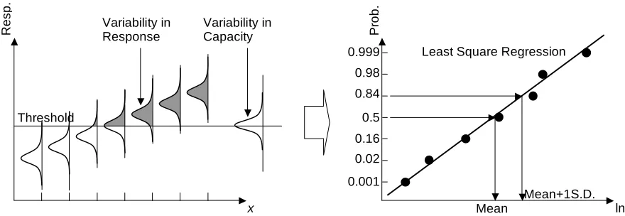
Eqns. (3) and (4) assume that response R(x) must be proportional to ground motion intensity x and log-normal standard deviation of response !R(x) must be constant though these assumptions are not realistic when considering strong nonlinear response. In order to avoid these unrealistic assumptions, Sato et al. (2006) evaluates !X and !X based on Monte-Carlo simulation as shown in Fig.1.
Figure 1. Procedure to evaluate single-valued fragility characteristics based on Monte-Carlo simulation
ln(x)
R
e
s
p
.
Threshold
Variability in Capacity Variability in
Response
Least Square Regression
Mean+1S.D. Mean
0.5 0.84
0.16 0.98
0.02
P
ro
b
.
0.999
0.001
3.2 Proposal of the vector-valued fragility analysis
3.2.1 Methodology to obtain vector-valued fragility
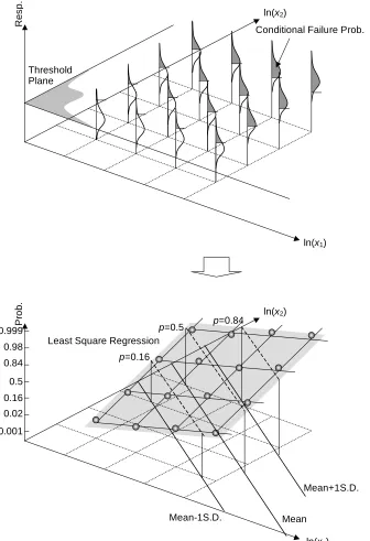
A vector-valued fragility is the extension of a single-valued fragility. The concept to evaluate vector-valued fragility is shown in Fig. 2 and the procedure is summarized as follows,
Step 1: Assign some combination of ground motion intensities x1 and x2,
Step 2: Evaluate probability density function of response for each combination of x1 and x2, Step 3: Evaluate conditional probability for each combination of x1 and x2, and,
Step 4: Perform regression analysis to obtain probabilistic characteristics of vector-valued fragility.
Figure 2. Procedure to evaluate vector-valued fragility characteristics based on Monte-Carlo simulation
Threshold Plane
Conditional Failure Prob.
R
e
s
p
.
ln(x1)
ln(x2)
P
ro
b
.
ln(x1)
ln(x2)
0.5 0.84
0.16 0.98
0.02 0.999
0.001
Least Square Regression
Mean
Mean+1S.D.
p=0.5
p=0.16
p=0.84
3.2.2 Effect of response spectral shape on ratio of PGA to PGV
In order to carry out the vector-valued fragility analysis illustrated in Fig.2, it is required to obtain ground motion possessing the given ratio of PGA to PGV. Since artificial ground motion is generated based on the given acceleration response spectrum in this study, the effect of response spectral shape on the ratio of PGA to PGV is examined.
In this study, the response spectral shape is characterized by three parameters, T1, T2 and X, which are shown in Fig.3. With these parameters, the response spectral shape is given by the following equations,
) 02 . 0 ( 02 . 0
0 . 1 0
. 1 ) (
1
! !
! +
= T
T X T
S ; 0.02!T<T1, (5a)
X T
S( )= ; T1!T <T2, and, (5b)
T T X T
S( )= ! 2 ; T !T
2 . (5c)
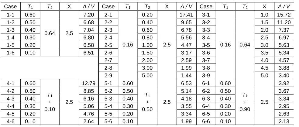
In Table1, the ratios of PGA to PGV for various combinations of parameters are summarized, followed by the following findings,
1. The effect of T1 is negligible,
2. The larger T2 is, the smaller the ratio of PGA to PGV is, 3. The larger X is, the smaller the ratio of PGA to PGV is, and, 4. The larger (T2 !T1) is, the smaller the ratio of PGA to PGV is.
Figure 3. Response spectral shape
Table 1. Effect of parameters on the ratio of PGA to PGV
Case T1 T2 X A / V Case T1 T2 X A / V Case T1 T2 X A / V
1-1 0.60 7.20 2-1 0.20 17.41 3-1 1.0 15.72
1-2 0.50 6.68 2-2 0.40 9.65 3-2 1.5 11.20
1-3 0.40 7.04 2-3 0.60 6.78 3-3 2.0 7.37
1-4 0.30 6.80 2-4 0.80 5.56 3-4 2.5 6.97
1-5 0.20 6.58 2-5 1.00 4.47 3-5 3.0 5.63
1-6 0.10
0.64 2.5
6.51 2-6 1.50 3.17 3-6 3.5 5.34
2-7 2.00 2.59 3-7 4.0 4.57
2-8 3.00 1.99 3-8 4.5 3.88
2-9 0.16
5.00 2.5
1.44 3-9
0.16 0.64
5.0 3.40
4-1 0.60 12.79 5-1 0.60 6.53 6-1 0.60 3.92
4-2 0.50 8.85 5-2 0.50 5.14 6-2 0.50 3.67
4-3 0.40 6.16 5-3 0.40 4.18 6-3 0.40 3.34
4-4 0.30 5.06 5-4 0.30 3.55 6-4 0.30 2.95
4-5 0.20 4.76 5-5 0.20 3.34 6-5 0.20 2.63
T1 + 0.10
2.5
T1 + 0.50
2.5
T1 + 0.90
2.5
0.02 T1 T2
1.0 X
10.0
A
m
p
lif
ic
a
ti
o
n
3.3 Application
3.3.1 Model structure and its characteristics
In application, 7-story RC frame building is employed, which is modelled as a lumped mass model with nonlinear springs. Nonlinear characteristics is a modified Takeda model with tri-linear skeleton Specification of analytical model is given according to the building standard law in Japan, as summarized in Table 2.
Table 2. Specification of model structure
Stiffness (tonf/m) Strength (tonf)
Level (m)
Weight
(tonf) Initial:k0 Post-cracking Post-yielding Yielding: Q Cracking
24.5 12668 98.5
21.0 17395 135.3
17.5 20820 161.9
14.0 23991 186.6
10.5 27000 210.0
7.0 29653 230.6
3.5
100.0
31780
k0/4 k0/100
247.2
Q/3
3.3.2 Generation of input ground motion
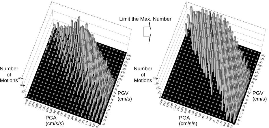
Input ground motions used in the Monte-Carlo simulation are generated according to the following conditions,
Condition 1: Range of T1 is 0.1 to 1.0 (sec.),
Condition 2: Range of T2 is 0.1 to 1.0 (sec.) under the condition that T1<T2, Condition 3: Range of X is 1.0 to 4.0, and,
Condition 4: Range of the PGA is 50-5000 (m/s/s).
After being generated, numerous input ground motions are put into 441 (21!21) bins as shown in Fig.4. It is noted that the maximum number of ground motions in each bin is 20 in case of the Monte-Carlo simulation.
Figure 4. Distribution of generated input ground motions
10 12
14 17
21 25
30 36
44 53
63 76
91 110
132 159
191 230277
333 400
10 0 120 145 17
4 209 251 30
2 364 43
7 52
6 63
2 76
1 915 11
00 13
23 159
1 191
3 23
00 276
6 332
6 40
00 0 5 10 15 20
!"#
PGV(cm/s)
PGA(cm/s/s) 10
12 14
17 21
25 30
36 44
53 63
76 91
110 132
159 191
230277 333
400
10 0 120 145 17
4 209 251 30
2 364 437 52
6 63
2 76
1 915 11
00 13
23 159
1 191
3 23
00 276
6 332
6 40
00 0 20 40 60
!"#
PGV(cm/s)
PGA(cm/s/s)
PGV (cm/s)
PGV (cm/s)
PGA (cm/s/s)
PGA (cm/s/s) Number
of Motions
Number of Motions
Generated Input Ground Motions Input Ground Motions for MCS
3.3.3 Result of Monte-Carlo simulation
In Fig.5, shown are the median of story drift angle and the log-normal standard deviation of it, since the story drift angle is employed as a measure of damage quantification. From the figure, it is seen that the median of story drift angle increases with increment in magnitude of PGA or PGV. On the contrary, no relationship among the log-normal standard deviation, PGA and PGV is observed.
Figure 5. Results of Monte-Carlo simulation
3.3.4 fragility analysis
The conditional failure probability p(a,v) is given by the following equation,
! " # $
% & '
=
) , (
} / ) , ( ln{ )
, (
v a
r v a r v
a p
( , (6)
where, a is PGA, v is PGV, r(a,v) is the median of story drift angle, !(a,v) is the log-normal standard deviation, r is the threshold regarding to drift angle, and "[!] is the normal distribution function. The threshold r is summarized in Table 3.
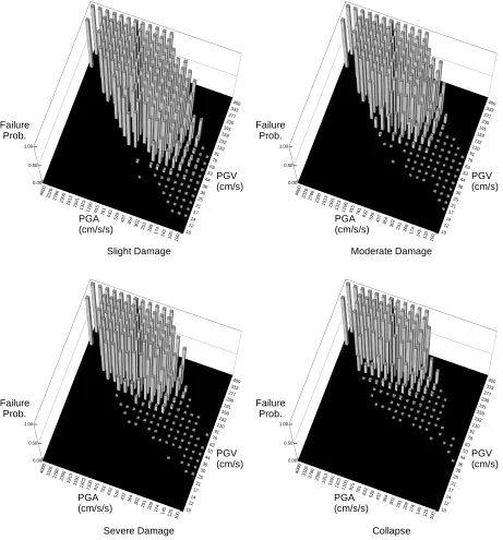
For each threshold, the conditional failure probability p(a,v) is obtained. In this study, p(a,v) is calculated for 441 (21!21) bins. The results are shown in Fig. 6.
Table 3. Threshold for each limit state
Limit state Drift angle
Slight damage 1/240
Moderate damage 1/120
Severe damage 1/60
Collapse 1/30
10 12
14 17
21 25
30 36
44 53
63 76
91 110
132 159
191230 277
333 400
10 0 120 145 17
4 209 251 30
2 364 43
7 526 63
2 76
1 915 11
00 13
23 159
1 191
3 23
00 276
6 332
6 40
00 0.00 0.05 0.10 0.15
!"#
PGV(cm/s)
PGA(cm/s/s) 10
12 14
17 21
25 30
36 44
53 63
76 91
110 132
159 191230
277 333
400
10 0 120 145 17
4 209 251 30
2 364 43
7 526 63
2 76
1 915 11
00 13
23 159
1 191
3 23
00 276
6 332
6 40
00 0 0.2 0.4 0.6 0.8
!"#
$%& PGV(cm/s)
PGA(cm/s/s)
PGV (cm/s)
PGV (cm/s)
PGA (cm/s/s)
PGA (cm/s/s)
Median Log-normal S.D.
Figure 6. Conditional failure probability based on Monte-Carlo simulation
3.3.5 Development of fragility plane
In case of single-valued fragility analysis, the logarithmic mean !X and logarithmic standard deviation !X are derived by regression analysis using the following equation,
X Xs
x=" +!
ln , s="!1[p(x)] (7)
where, p(x) is the conditional failure probability for the given ground motion intensity x.
In case of vector-valued fragility analysis, however, it is impossible to determine logarithmic means, since PGA and PGV are in the relationship of trade-off. So, eqn. (7) is rewritten as follows,
X X X x s ! " ! #
= 1 ln . (8)
10 12 14 17 21 25 30 36 44 53 63 76 91 110 132 159 191 230277 333 400
100 12 0 14 5 17 4 20 9 251 30
2 364 437 52
6 632 761 91
5 110
0 132
3 15
91 19
13 230
0 27 66 33 26 40 00 0.00 0.50 1.00 !" #$ PGV(cm/s) PGA(cm/s/s) 10 12 14 17 21 25 30 36 44 53 63 76 91 110 132 159 191 230277 333 400
100 12 0 14 5 17 4 20 9 251 30
2 364 437 52
6 632 761 91
5 110
0 132
3 15
91 19
13 230
0 27 66 33 26 40 00 0.00 0.50 1.00 !" #$ PGV(cm/s) PGA(cm/s/s) 10 12 14 17 21 25 30 36 44 53 63 76 91110 132 159 191 230277 333 400
100 12
0 14
5 174 20
9 251 30
2 364 437 52
6 632 761 91
5 110
0 132
3 15
91 19
13 230
0 27 66 33 26 40 00 0.00 0.50 1.00 !" #$ PGV(cm/s) PGA(cm/s/s) 10 12 14 17 21 25 30 36 44 53 63 76 91110 132 159 191 230277 333 400
100 12
0 14
5 174 20
9 251 30
2 364 437 52
6 632 761 91
5 110
0 132
3 15
91 19
13 230
0 27 66 33 26 40 00 0.00 0.50 1.00 !" #$ PGV(cm/s) PGA(cm/s/s) Failure Prob.
Severe Damage Collapse
PGA (cm/s/s) PGA (cm/s/s) PGA (cm/s/s) PGA (cm/s/s) PGV (cm/s) PGV (cm/s) PGV (cm/s) PGV (cm/s) Failure Prob. Failure Prob. Failure Prob.
Instead of giving explicit form of probability characteristics, eqn. (8) can give the conditional probability for ground motion intensity x.Eqn. (8) is now extended as follows,
!! " # $$
% &
+
'
+ =
V V A A V
A
v a
s
( ) (
) (
( ln
1 ln 1
, (9)
where, a is PGA, v is PGV, respectively. It is noted that neither !A nor !V are evaluated separately. By setting s=0, the median capacity, which is the value in the parentheses in eqn. (9), is obtained by the following equations,
v a
V A
V V A
A 1 ln 1 ln
! !
! " !
" = +
## $ % &&
'
( +
. (10)
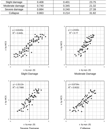
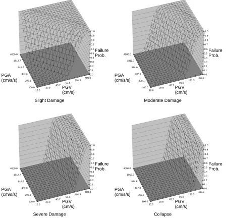
Results of regression analysis are summarized in Table 4. Comparison of probability characteristic value s by Monte-Carlo simulation and that by eqn. (9) is shown in Fig. 7. With these regression coefficients, fragility planes are developed using eqn. (10), as shown in Fig. 8.
Table 4. Results of regression analysis
Limit state A v ( A/ A+ V/ V)
Slight damage 0.408 0.401 23.75
Moderate damage 0.740 0.345 21.32
Severe damage 0.884 0.240 27.39
Collapse 0.863 0.214 31.82
y = 0.8193x R2 = 0.8491
-5 0 5
-5 0 5
s by eqn. (9)
s
b
y
M
C
S
y = 1.1533x R2 = 0.77
-5 0 5
-5 0 5
s by eqn. (9)
s
b
y
M
C
S
y = 1.0113x R2 = 0.7988
-5 0 5
-5 0 5
s by eqn. (9)
s
b
y
M
C
S
y = 0.8734x R2 = 0.8032
-5 0 5
-5 0 5
s by eqn. (9)
s
b
y
M
C
S
Slight Damage Moderate Damage
Figure 8. Developed fragility planes
4
DISCUSSION
From Fig. 7, it can be seen that both PGA and PGV are adequate as ground motion measure for limit state of slight damage, since the inclinations of hazard plane in both direction are identical. This corresponds to the fact that regression coefficients !A and !V are almost same. For limit states of moderate damage, severe
damage and collapse, PGV can be better measure than PGA. This is observed both in regression coefficients and in inclination of fragility plane. The severer the limit state is, the stronger this tendency is.
In general, PGA is suitable for short-period structure and PGV is suitable for long-period structure. So, above tendency is compatible with the fact that severer damage gives the structure longer period.
In case of single-valued fragility analysis, the ground motion measure employed may not be adequate for every limit states of concern. Also it may not be adequate when carrying out the risk analysis of portfolio consisting of various types of buildings. Vector-valued fragility can be the solution for the problems, since vector-valued fragility possesses the both characteristics of PGA and PGV.
10.0
20.9 43.7
91.5 191.3 400.0
100.0 209.1 437.3 914.6 1912.7 4000.0
0.0 0.1 0.2 0.3 0.4 0.5 0.6 0.7 0.8 0.9 1.0
!"#$
PGV(cm/s) PGA(cm/s/s)
10.0
20.9 43.7
91.5 191.3 400.0
100.0 209.1 437.3 914.6 1912.7 4000.0
0.0 0.1 0.2 0.3 0.4 0.5 0.6 0.7 0.8 0.9 1.0
!"#$
PGV(cm/s) PGA(cm/s/s)
PGV (cm/s)
PGV (cm/s) PGA
(cm/s/s)
PGA (cm/s/s) Failure
Prob.
Failure Prob.
Moderate Damage Slight Damage
10.0
20.9 43.7 91.5
191.3 400.0
100.0 209.1 437.3 914.6 1912.7 4000.0
0.0 0.1 0.2 0.3 0.4 0.5 0.6 0.7 0.8 0.9 1.0
!"#$
PGV(cm/s) PGA(cm/s/s)
10.0
20.9 43.7
91.5 191.3 400.0
100.0 209.1 437.3 914.6 1912.7 4000.0
0.0 0.1 0.2 0.3 0.4 0.5 0.6 0.7 0.8 0.9 1.0
!"#$
PGV(cm/s) PGA(cm/s/s)
PGV (cm/s)
PGV (cm/s) PGA
(cm/s/s)
PGA (cm/s/s) Failure
Prob.
Failure Prob.
5
CONCLUSION
In this paper, the seismic fragility analysis using PGA and PGV as ground motion measure is proposed. In constructing the procedure, the effects of response spectral shape on the ratio of PGA to PGV is examined so that the numerous input ground motions for Monte-Carlo simulation can be generated. By applying the method to model structure that is 7-story RC frame building, followings are obtained.
By expressing probability characteristic value s as a function of PGA and PGV, seismic fragility plane can be obtained.
Though both PGA and PGV are adequate as ground motion measure for slight damage, PGV is preferable for severer damage in which the natural period of structure gets larger due to inelastic behaviour.
REFERENCES
Bazzurro P, Cornell CA.2002. Vector-valued probabilistic seismic hazard analysis(VPSHA). Proceedings 7th U.S. National Conference on Earthquake Engineering. Boston. MA.
Fukushima S., Hayashi T., Yashiro H. 2007. Seismic hazard analysis based on the joint probability density function of PGA and PGV. Transaction of 19th SMiRT. Paper No.M03/1.
Sakai Y., Yoshioka S., Koketsu K., Kabeyasawa T. 2001. Investigation on indices of representing destructive power of strong ground motions to estimate damage to buildings based on the 1999 Chi-Chi earthquake, Taiwan. Journal of structural and construction engineering. Transaction of AIJ. P 43-50. (in Japanese)
Sato I., Yashiro H., Ota K., Fukushima S. 2006. Fragility curves for any damage state based on capacity index. Proc. of 100th Anniversary Earthquake Conference. CD-ROM.
Sato Y., Fukushima S., Yashiro K. 1995. Study on the index of seismic motion for fragility analysis. Summaries of technical papers of Annual Meeting AIJ. B-1. P 21-22. (in Japanese)