Copyright2000 by the Genetics Society of America
Understanding the Overdispersed Molecular Clock
David J. Cutler
Center for Population Biology, University of California, Davis, California 95616
Manuscript received April 23, 1999 Accepted for publication December 2, 1999
ABSTRACT
Rates of molecular evolution at some protein-encoding loci are more irregular than expected under a simple neutral model of molecular evolution. This pattern of excessive irregularity in protein substitutions is often called the “overdispersed molecular clock” and is characterized by an index of dispersion, R(T)⬎ 1. Assuming infinite sites, no recombination model of the gene R(T) is given for a general stationary model of molecular evolution. R(T) is shown to be affected by only three things: fluctuations that occur on a very slow time scale, advantageous or deleterious mutations, and interactions between mutations. In the absence of interactions, advantageous mutations are shown to lower R(T); deleterious mutations are shown to raise it. Previously described models for the overdispersed molecular clock are analyzed in terms of this work as are a few very simple new models. A model of deleterious mutations is shown to be sufficient to explain the observed values of R(T). Our current best estimates of R(T) suggest that either most mutations are deleterious or some key population parameter changes on a very slow time scale. No other interpretations seem plausible. Finally, a comment is made on how R(T) might be used to distinguish selective sweeps from background selection.
T
HE most simple version of the neutral theory of phylogeny. The numbers of amino acid substitutionsalong all branches in the phylogeny were inferred. Next,
molecular evolution (Ohta and Kimura 1971;
Sawyer1977;Kelly1979;Kimura1983) predicts that the branch lengths and mutation rates were found by
a maximum-likelihood method. Finally, a2(Langley
the number of mutations that arise in a population in
T generations, which ultimately become fixed in the andFitch1973) and a likelihood-ratio test (Langley
andFitch 1974) were performed to ask whether the population, will be Poisson distributed with mean uT,
where u is the per sequence, per generation mutation observed numbers of mutations on the branches were
statistically different from the expected. The neutral rate. Therefore, the variance in the number of
substitu-Poisson model was rejected with high confidence. Two tions will equal the mean under this most simple neutral
basic interpretations of Langley and Fitch have been model. The ratio of the variance in the number of
substi-offered. The first interpretation suggested that the rate tutions to the mean number is called the index of
disper-of molecular evolution changed over time (Langley
sion of molecular evolution. Under the most simple
andFitch1974); i.e., the mean number of substitutions neutral theory, the index of dispersion, R(T), should
was not constant over time (the substitution process is equal 1.
not stationary). The second interpretation (Gillespie
The first article to demonstrate a deviation from a
andLangley1979) was that the mean number of substi-Poisson number of substitutions occurred early in the
tutions remained constant over time (the substitution
history of the neutral theory (OhtaandKimura1971).
process was stationary), but that the variance in the Ohta and Kimura examined three proteins in several
number of substitutions was larger than would be pro-pairwise comparisons in mammals. They showed that
duced by a Poisson process, i.e., the index of dispersion for two of the proteins in a few of the pairs, a Poisson
was larger than one. substitution rate could be rejected. This result was hard
In 1983, Kimura attempted to directly test whether or to interpret, as no explicit phylogenetic hypothesis was
not the index of dispersion truly equaled one (Kimura
made, and the effect of phylogeny went unconsidered.
1983). Kimura considered four different proteins taken The first attempts to use a phylogeny in an explicit
from six mammalian lineages. He assumed these six
manner came a few years later (Langley and Fitch
lineages came from a star phylogeny, and therefore the 1973, 1974). Langley and Fitch examined four proteins
number of substitutions in each lineage was an indepen-in 18 species. The species were assumed to have a known
dent sample, each with mean uT. He calculated R(T) for each of these four proteins and found that R(T) ranged between 1.7 and 3.3. Although R(T) was bigger
Address for correspondence: Department of Genetics, Rm. BRB 747B,
than predicted, in only two of the proteins was it
signifi-Case Western Reserve University, 2109 Adelbert Rd., Cleveland, OH
44106-4955. E-mail: [email protected] cantly larger than one.
In a series of articles,Gillespie(1984a, 1986a,b) ex- is larger than one for both silent and replacement sites. This “overdispersion” is not due to lineage effects and tended Kimura’s test to nine proteins (both nuclear
and mitochondrial), but again assumed a mammalian is not an artifact of correction formulas. The conclusion
is inescapable. For mammals, the most simple neutral
star phylogeny. Gillespie (1986b) found that R(T)
ranged from 0.16 to 35.55, and he had more than theory of molecular evolution does not explain protein
divergence data. enough observations to repeatedly reject the most
sim-ple neutral theory. Despite the rather clear rejection of A recent study of Drosophila (Zeng et al. 1998) has
cast some doubt on whether conclusions drawn from the simple neutral model, this analysis was less than
completely convincing for several reasons. First, a star mammalian data should necessarily be applied to all
life. Zeng and colleagues examined 24 proteins from phylogeny was assumed. If this assumption were false,
individual lineages would have different T ’s, and the three species of Drosophila, Drosophila pseudoobscura, D.
subobscura, and D. melanogaster. D. pseudoobscura and D.
variance would be artificially inflated (Gillespie1989).
Second, under the neutral theory, the substitution rate subobscura are relatively closely related, with D.
melanogas-ter a more distantly related out-group. They found that, should only be constant per generation, so different
length generations in different lineages should artifi- using Gillespie’s weighting factor, averaged over these
24 loci, R(T) was 4.37 for silent sites but only 1.64 for
cially inflate R(T) (Gillespie1989). Third, an overall
increase or decrease in the mutation rate in only some replacement sites. The value obtained for silent sites
was qualitatively in agreement with Ohta’s value for of the lineages (perhaps due to a systemic change in
metabolic rate or in DNA repair machinery, etc.) would mammals, but the replacement values were much
smaller and not statistically different from 1.
Unfortu-lead to an artificial inflation of R(T) (Gillespie1989).
Fourth, in certain circumstances use of a correction nately, interpretation of the replacement site results is
confounded by extremely low replacement divergence formula to estimate divergence distances could
artifi-cially inflate R(T) (Bulmer1989;Gillespie1989). Gil- between D. pseudoobscura and D. subobscura (see
discus-sionbelow).
lespie solved the first three problems, collectively known
as lineage effects, in 1989. It now seems clear that mammalian loci are, on
aver-age, overdispersed at both silent and replacement sites. Gillespie’s solution to lineage effects was to (1) restrict
his analysis to three species at a time, thereby guarantee- In Drosophila, it is likely that silent sites are
over-dispersed, but replacement sites might not be. In any ing a single unrooted phylogeny, and (2) weight the
number of substitutions in each lineage by one over the case, because the most simple neutral theory can never
produce an R(T) ⬎ 1, it is of interest to know which
mean number for that lineage, where the mean is taken
over all loci examined. This weighting process amounts models of molecular evolution can produce a large
in-dex of dispersion. Several models have been suggested. to regressing out lineage effects from the data. Using
these weightings, Gillespie showed that for replacement They include episodic selection on a mutational
land-scape (Gillespie1984a,b, 1991), the fluctuating neutral
substitutions in 20 loci, R(T) ranged from 0.13 to 43.82
with a mean of 6.95 (Gillespie 1991, p. 119). Silent space model (Takahata1987, 1989), and the house of
cards (HOC) model of slightly deleterious mutations sites at these same loci had an average R(T) of 4.64.
Gillespie concluded that R(T) was clearly statistically (OhtaandTachida1990;Tachida1991;Iwasa1993;
Gillespie 1994b;Tachida 1996;ArakiandTachida
significant for replacement sites, but was perhaps only
marginally significant for silent sites, due to the bias 1997). In addition to these particular models, there
is an extensive set of simulations by Gillespie (1993,
introduced by use of correction formulas.
Goldman (1994) quantified the extent of the error 1994a,b), which tried to characterize R(T) for numerous models. With these simulations, Gillespie showed that lineage effects might have introduced in the early
esti-mates of R(T). He further noted that Gillespie’s simula- fluctuating selection could account for a high index of
dispersion, but only if the fluctuations occurred very tions of his weighting factor solution had not been as
extensive as they could have been. Nielsen more than slowly, roughly at the same rate fixations happened
(Gillespie1993). In addition, he found that symmetric
made up for this lack of simulations (Nielsen 1997)
and further showed that the fourth problem due to underdominance (Gillespie1994a), optimizing
selec-tion, and the house of cards model (Gillespie1994b)
correction formulas was not very large as long as the
sequences were not too close to saturation. could all produce R(T)⬎1, but only in a very narrow
range of parameter values. He found that exponential By 1995 enough data had been gathered to examine
49 mammalian loci. Using Gillespie’s weighting factor, and gamma shift models of deleterious sites produced
R(T)≈1 (Gillespie1994b) (Table 1).
Ohta(1995) showed that, averaged over all these loci,
R(T)⬎ 5 for both silent and replacement sites. These In other simulations,Gillespie(1994a) showed that
rapidly fluctuating selection not only failed to explain values were more than large enough to reject simple
neutrality. So taken as a whole, the evidence from mam- a large index of dispersion, but actually produced an
R(T) ⬍ 1. This result was particularly surprising. Put
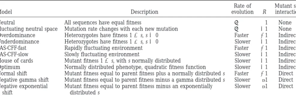
TABLE 1
Previously described models
Rate of Mutant site
Model Description evolution R interaction
Neutral All sequences have equal fitness 1 None
Fluctuating neutral space Mutation rate changes with each new mutation ⬎1 None Overdominance Heterozygotes have fitness 1⫹s, s⬎0 Faster ⬍1 Indirect Underdominance Heterozygotes have fitness 1⫺s, s⬎0 Slower ⬎1 Indirect SAS-CFF-fast Rapidly fluctuating environment Faster ⬍1 Indirect SAS-CFF-slow Slowly fluctuating environment Slower ⬎1 Indirect House of cards Mutant fitness 1⫹s, with s normally distributed Slower ⬎1 Indirect Optimum Normally distributed phenotype, quadratic fitness function Slower ⬎1 Indirect Normal shift Mutant fitness equal to parent fitness plus a normally distributed s Faster ⬍1 Direct Negative gamma shift Mutant fitness equal to parent fitness minus a gamma distributed s Slower ≈1 Direct Negative exponential Mutant fitness equal to parent fitness minus an exponentially Slower ≈1 Direct
shift distributed s
only a little bit facetiously, Gillespie took a neutral infinite number of sites and by assuming that there
is no recombination between those sites (Watterson
model, added some random fluctuations to it, and
de-rived a process that was less random than the one he 1975). Assume that time is discrete and that population
size is constant and equal to N⬍∞haploid individuals.
started with. Other models also produced R(T) ⬍ 1,
including symmetric overdominance and normal shift Let the population reproduce according to a discrete
time Moran model (Moran1958). The mutation
pro-models. Gillespie attempted to develop some insight
concerning how a model might produce an R(T)⬍ 1 cess and site frequency dynamics are assumed to be
stationary, so that translations of the time axis do not (Gillespie1993), but his insight was built by
consider-ing an infinite allele, not an infinite site model. It is effect the origination process. Let Mtequal one if there
is a mutation at time t, and equal zero otherwise. Let St
argued below that infinite site models behave
substan-tially differently than infinite allele models, and his re- equal one if there is an origination at t, and zero
other-wise. It can be shown that ratio of the variance in the sult is only applicable to the latter. The mechanism by
which an infinite site model could ever produce an R(T) number of originations, divided by the mean number
of originations in T time steps, R(T), is given by
⬍1 has not yet been suggested.
The goals of this article are threefold: first, to describe
the mathematical machinery necessary to analyze the R(T)⫽ Var
兵
RT t⫽1St
其
E
兵
RT t⫽1St其
index of dispersion for an infinite site model of the gene and second, using this machinery, to describe
⫽ 1⫺ ⫹2
兺
T
t⫽1
冢
1⫺T冣t (h(t)⫺ ) (1)
which models will produce R(T)⬎1, which will produce
R(T) ⬍ 1, and which will produce R(T) ≈ 1. Finally,
from our observation that R(T) appears to be ⬎5 for
(Cutler 2000), where is the origination rate, ⫽ mammalian data, this article attempts to discover what
E{St} ⫽ Pr{St⫽ 1}, and h(t) is the conditional intensity
we can infer about the nature of mammalian evolution.
function defined by
h(t)⫽Pr{St⫽1|S0⫽1}. (2)
CALCULATION OF R(T)
Equations 1 and 2 are discrete time analogs of results
A substitution is a mutation that ultimately fixes in given by Cox and Isham (1980, Equations 2.27 and
the population. There are two different processes that 1.19). It can be shown that (2) can be rewritten (Cutler
might be called the substitution process. One process, 2000) as
the origination process (Gillespie1994a), is the point
h(t)⫽Pr{M0⫽ 1|Mt⫽1}᐀(t)E{Xt}, (3)
process of the times of entry of those mutations that
ultimately fix in the population. The other process, the where E{X
t} is the expected frequency of a mutant t time
fixation process (Gillespie1994a), is the point process steps after it enters the population, and ᐀(t) is the
of the times when mutations, which ultimately fix, first amount of interaction between sites separated by t time
reach frequency one. This article is concerned only with units, defined by
the origination process.
To derive the index of dispersion of the origination ᐀(t)⫽ Pr{St⫽1|jt on i0}
p , (4)
where p is the probability of fixation of a new mutant, cesses that are often considered slow (for instance glaci-ation) are usually orders of magnitude faster than would p⫽E{St|Mt⫽1}, and jton i0is the condition of a mutant
arising at time t on a piece of DNA containing a mutant be required here. To fully explain R(T), a mechanism
would need to be suggested that could cause a key pa-that arose at time 0.
If h(t) converges to sufficiently quickly, so that rameter to change so slowly. Without such a mechanism,
a slowly changing environment appears a somewhat
hol-R∞t⫽1t(h(t) ⫺ ) ⬍ ∞, then for large T, R(T) can be
approximated by low explanation.
Takahata’s fluctuating neutral space (FNS) model R∞⫽lim
T→∞
R(T)⫽ 1⫺ ⫹2
兺
∞
t⫽1
(h(t) ⫺ ) (5) (Takahata1987, 1989) could provide a possible
mech-anism. At the heart of the FNS model is the notion that
≈1⫹2Ds, (6) each mutation changes the subsequent mutation rate
for a given piece of DNA. This process is difficult to
where Ds ⫽R∞1(h(t)⫺ ). The approximation uses the model exactly [seeCutler(2000) for an attempt], so
fact that Ⰶ 1. The sign of Ds determines whether it is often approximated by a model where mutation
the substitutional process is overdispersed (Ds ⬎ 0), rate changes with each substitution (Takahata1987,
underdispersed (Ds ⬍ 0), or indistinguishable from a 1989; Cutler 2000). Whether this change occurs at
neutral model (Ds⫽0). Thus Dscan be thought of as the moment a mutant first reaches frequency one (i.e.,
the deviation in R(T) from a simple neutral model. It corresponding to events in the fixation process), or at
turns out that Ds can be calculated directly for a few the moment a mutant destined to fix first enters the
simple models. Even when direct calculation of Ds is population (i.e., corresponding to events in the
origina-difficult, its sign and relative magnitude can often be tion process) is often left obscured by the coarseness
estimated. of the approximations used in the analysis (Takahata
A few comments concerning the conditional intensity 1987;Cutler2000). Regardless of the modeling details,
function should be made. It is defined to be the product the FNS model has the property the mutation rate must
of three terms, the probability there is a mutation at change on the same time scale as molecular evolution.
time 0, given a mutation at time t, Pr{M0 ⫽1|Mt ⫽ 1}, Therefore, the FNS model is capable of generating large
the expected frequency of a mutant t time units after R(T) values. Several results on the FNS model have been
it entered the population, E{Xt}, and the amount of obtained.
interaction between mutants separated by t time steps, First, for the FNS model to generate large values of
᐀(t). The amount of interaction between mutants,᐀(t), R(T), there must be more than two possible mutation
is defined to be the probability of fixation of a mutant, rates (Cutler2000). Second, when new mutation rates
given that it occurred on a piece of DNA containing a are picked independently of previous rates, R(T) ⫽5
mutation that entered the population t time steps ear- implies that sequences that differ by only a single site will
lier, Pr{St ⫽ 1|jt on i0}, divided by the unconditional have mutation rates that differ by an order of magnitude
probability of fixation of a mutant p. A more complete 2–5% of the time (depending on the details of the
description of ᐀(t) is given below. distribution of mutation rates;Cutler2000). Processes
where new mutation rates are not independent of
previ-ous rates are difficult to analyze (Takahata1989), but
SLOWLY CHANGING ENVIRONMENT
can produce large values of R(T), if the process has a
sufficient amount of time to evolve (Takahata1989).
Virtually any model containing a key parameter that changes on a sufficiently slow time scale can explain the observed index of dispersion. Other work has shown
UNDERSTANDING MODELS WITH SELECTION
(Cutler2000) that if either the mutation rate or the
probability of fixation changes as slow as, or slower than, Many models make the assumption that the mutation
the average time between fixation of sites, then the process has a constant rate. If(t) ⫽ , then
index of dispersion can be elevated significantly above
one.Gillespie’s (1993) simulations confirm that mod- R∞≈1⫹2
兺
∞t⫽1
(᐀(t)E{Xt}⫺p). (7)
els of a slowly fluctuating environment can produce
large R(T)’s regardless of the details of the model. If there is little interaction between sites (᐀(t) ≈ 1),
Despite the fact that slowly changing parameters can then (7) further reduces to
cause R(T) to be large, simply invoking slow change
appears to be an incomplete explanation of R(T). If R
∞ ≈1⫹ 2
兺
∞
t⫽1
(E{Xt}⫺p) (8)
one assumes that the time between substitutions is
mea-sured in millions of years, one must also assume that ⫽ 1⫹D
s1,
the environment changes on the time scale of millions
of years. At first glance, it is not obvious that any environ- where Ds1⫽2R∞t⫽1(E{Xt}⫺p) can be thought of as the
pro-mutation interactions. In many cases, understanding Ds1 from time step ⫺1. The probability that there was a
is the key to understanding selection’s effect on the mutation at time⫺1 is. The probability that i0contains
index of dispersion. this mutation is E{X1} (BirkyandWalsh1988;Cutler
The expected frequency of a neutral mutation does 2000). Because no more than one mutation can occur
not change over time; E{Xt1} ⫽E{Xt2}⫽ p for all t1 and in a single time step,E{X1} is the expected number of
mutations on i0from time step ⫺1. SimilarlyE{X2} is
t2. Nonneutral mutations do not necessarily have this
the expected number of mutations from time step⫺2.
property. Ds1measures the effect a changing expected
In general, the first sum in (9) is the expected number frequency has on the index of dispersion. A simple rule
of mutations on i0.
of thumb results. In the absence of site interactions,
In a neutral model, the expected frequency of a site
deleterious mutations cause R(T) ⬎ 1, and
advanta-does not change over time. So, for a neutral model
geous mutations cause R(T)⬍1. The magnitude of the
E{Xt}⫽p for all t. Thus, the second sum in Equation 9
effect can be made quite large.
is what the expected number of mutations on i0would
The overall sign of Ds1 is obviously determined by
be, if this were a neutral model with probability of
fixa-the sign of fixa-the E{Xt}⫺ p. If the expected frequency of
tion p. Therefore, Ds1/2 is equal to the expected number
mutations does not change over time, then Ds1⫽ 0. If
of mutations on i0minus the expected number of
muta-the expected frequency of sites monotonically declines
tions under a neutral model. For a deleterious site
over time, then Ds1 ⬎ 0 [because E{Xt} ⱖ E{X∞} ⫽ p,
model E{Xt}⬎p, so that the first sum is bigger than the
E{Xt} ⫺ p ⱖ 0]. Conversely, if the expected frequency
second, and, on average, there are“too many” mutations
monotonically increases, then Ds1 ⬍ 0. An interesting
on i0, relative to a neutral model with the same
probabil-unsolved problem is to describe which models of
molec-ular evolution have the property that the expected fre- ity of fixation. Conversely, in an advantageous model
quency of mutations is monotonic over time. A natural E{Xt} ⬍ p, so that there are “too few” mutations on i0
conjecture (and one that is consistent with the simula- relative a neutral model with the same probability of
tions performed here) is that any stationary model has fixation.
this property. Finding Ds1 directly for any particular model is not
Apart from a simple one-locus, two-allele Fisher-Wright trivial. Other than for the neutral case, it is not obvious
world, there is some difficulty defining what is meant that E{Xt} is ever easy to calculate. For models that may
by a deleterious/advantageous mutation. For the pur- be approximated with a diffusion, finding E{Xt} amounts
poses of this article, a particular mutation will be said to to solving a Kolmogorov backward equation. If a
two-be deleterious/advantageous if its expected frequency allele model is an adequate approximation, the problem
decreases/increases over time. A model will be said to can also be formulated as an ordinary differential
equa-be a deleterious/advantageous mutation model if, aver- tion (Ohta and Kimura 1969), but truncation of
aged over all possible mutants, the expected frequency higher-order moments is often necessary. Despite these
of mutants decreases/increases. Note that the definition difficulties, Ds1can be directly measured in a simulation.
of deleterious/advantageous mutation model is a prop- To estimate Ds1 within a simulation, a single extra
erty of the mutations, not the originations. Thus, a vector, call it DS[0 . . . R], needs to be stored, where R is
model will be called a deleterious site model if the a number sufficiently large so that all sites are extremely
majority of mutations decline in frequency, but this likely to be fixed or lost within R generations (R ⫽
statement implies nothing at all about the fitness of the 1000N was used in the simulations for this article).
Ini-sites that actually fix. It is a statement about the average tialize the DS vector to 0. During the simulation, track
properties of mutants, not a statement on the properties the frequency of each site in all generations. For each
of those rare mutants who eventually fix. mutation add its frequency t generations after it entered
Thus, we arrive at the conclusion that, in the absence the population to the value stored in DS[t]. When the
of site interactions, deleterious mutation models have simulation is done, divide each element of DS by the
an R(T)⬎1, and advantageous mutation models have total number of mutations. Estimate Ds1 by Ds1 ⫽
an R(T)⬍1. Although this result is clear as stated, the 2(RR
t⫽0DS[t] ⫺DS[R]).
intuition concerning why it’s true may be less obvious. Finally, one might ask if there is any general intuition
Mutations do not necessarily fix one at a time. Ds1 on the effects of the overall mutation rate and overall
can be thought of as measuring the effect the size and strength of selection on Ds1. As is obvious from Equation
frequency of multiple fixations has on the index of 8, Ds1is independent of time. Also, Ds1appears to be a
dispersion. To see this, write Ds1as: linear function of the mutation rate. For small mutations
rates, this may be roughly true, but for large 2 the
Ds1⫽2
冤
兺
∞
t⫽1
E{Xt}⫺
兺
∞
t⫽1
p
冥
. (9) linear dependence must disappear. The reason for thisis that E{Xt} and p must also be a function of 2, because
2effects, among other things, the overall
heterozygos-Consider the piece of DNA that reproduces at time step
Ds1is unlikely to depend on 2in a simple linear manner. knowledge that a piece of DNA contains an earlier
muta-tion can still indirectly effect the mutamuta-tion’s chance of By analogy to a classical Fisher-Wright model, one
can imagine changing the strength of selection. This fixation.
If one knows that jt arose on a piece of DNA
con-can have two effects on Ds1. First, it can change the
probability of fixation, p, thereby making p closer to/ taining i0, one has some information about the state
of the population. In particular, one suspects that i0’s
further from the initial frequency of a new mutant
(1/N), thereby decreasing/increasing |Ds1|. Second, expected frequency, conditional on jt arising on i0, is
higher than its unconditional expected frequency. The when the strength of selection changes, the time it takes
for the expected frequency to reach p will also change. knowledge that i0is expected to be at higher frequency
may, in turn, suggest something about the expected
Increasing selection decreases the time, so that |Ds1|
decreases. Decreasing selection increases the time, so mean fitness of the population. The expected mean
fitness of the population may, in turn, suggest some-that|Ds1|increases. Predicting the net effect is difficult.
In all the simulations, increasing selection usually in- thing about the probability that jt will fix. In general,
when i0 effects jt’s probability of fixation through one
creased |Ds1|, and never significantly decreased it, but
for very strong selection, Ds1generally appeared to ap- or more intermediaries (like population mean fitness),
we say that i0and jtindirectly interact. Virtually all
non-proach some asymptote.
neutral models should have some form of indirect inter-actions, although we suspect that models that produce
INTERACTION BETWEEN SITES
relatively constant population mean fitnesses might have relatively negligible indirect interactions.
Consider a mutant that enters the population at the
current time step, t. Call this mutation jt. The probability A simple rule of thumb can be applied to site
interac-tions. In general, direct interactions tend to move R(T)
that jtultimately fixes is p. When jtentered the
popula-tion, it arose on some piece of DNA. The piece of DNA toward one; indirect interactions tend to move R(T)
away from one. This can be seen by considering a few might contain other mutations. Pr{St⫽1|jton i0} is the
probability that jtfixes, given that the piece of DNA on simplified cases.
Consider an advantageous mutation model where the
which it arose contains another mutant, i0, which
en-tered the population at time zero. If knowing that the fitness of a piece of DNA with k mutations is equal to
1⫹ ks, s⬎ 0. This is, by definition, a model of direct piece of DNA contains an earlier mutation does not
effect jt’s chance of fixation, then Pr{St⫽1|jton i0} will interactions. If interactions were absent, R(T) would be
⬍1. Direct calculation of ᐀(t) is hard, but it has to
equal p, and᐀(t)⫽1. When᐀(t)⫽1 we say there is
no interaction between mutants. On the other hand, be ⬎1. Because all mutations are advantageous, the
probability of a site fixing, given that it arises on a piece
when the knowledge that jt arose on a piece of DNA
containing i0 alters the probability that jt fixes, we say of DNA containing another mutant, must be larger than
its unconditional probability of fixation, because its
fit-that there is interaction between mutants, and᐀(t)⬆1.
There are at least two fundamental ways in which ness is higher. So, ᐀(t)⬎ 1, which implies that when
E{Xt} ⬍p, ᐀(t)E{Xt}⬎ E{Xt}. Thus, when mutations are
mutants can interact. We call these two ways direct and
indirect interactions. For many models of natural selec- beneficial, direct interactions move R(T) toward 1.
The converse is true for the deleterious model with tion, the fitness of a piece of DNA is proportional to
the number of mutations that it contains. For instance, direct interactions. If the fitness of a sequence with k
mutations is 1 ⫺ ks, s ⬎ 0, then E{Xt} ⬎ p, and in the
in the negative gamma shift model (described below),
when a new mutation enters the population, the fitness absence of interactions, R(T) would be⬎1. But, because
each additional mutation lowers the fitness of a piece of the piece of DNA on which it arose is equal to its
fitness prior to the mutation, minus a gamma-distrib- of DNA, Pr{St⫽1|jton i0} must be less than p, and᐀(t)
must be⬍1. Thus, this form of direct interaction must
uted random variable. When the fitness of a piece of
DNA is a function of the number of mutations contained move R(T) toward 1.
Indirect interactions often have the opposite effect. on the piece of DNA, we say that mutations directly
interact with one another. Consider a mutation jt, which enters the population at
time t, on a piece of DNA containing an earlier mutation For other models of evolution, the fitness of a piece
of DNA containing a new mutation is independent of i0. Conditional on jt landing on a piece of DNA
con-taining i0, i0’s expected frequency is likely to be higher
the number of previous mutations. In the house of cards
model, the fitness of a piece of DNA containing a new than its unconditional expected frequency. If this is
a deleterious mutation model, i0’s higher conditional
mutation is drawn independently from some fixed
[of-ten Gaussian (Gillespie1994b;Tachida1996)] distri- expected frequency suggests that the conditional
ex-pected population mean fitness is likely to be lower than bution. Thus, the fitness of a piece of DNA containing
a new mutation is independent of the number of earlier the unconditional expectation. Given that jt arose at a
time when the conditional population mean fitness is mutations it contains. In this case, we say there is no
fitness, jt’s probability of fixation is likely to be higher, amounts of indirect interactions in the overdominance
model, because Gillespie has shown that the
homozygos-thereby making᐀(t)⬎1. Conversely, if this is an
advan-tageous mutation model, jt arising on i0 suggests that ity, and as a result mean fitness, changes very little over
time. There is likely to be a great deal more indirect the conditional expected population mean fitness may
be higher than the unconditional average, making it interaction in the underdominance model, because this
model does not maintain polymorphism, and there are
likely that jt’s probability of fixation is lower than the
unconditional average, so that ᐀(t) ⬍ 1. Therefore, significant changes in mean fitness as sites go to fixation.
Indirect interactions should reinforce the effects of ad-indirect interactions are likely to increase R(T) for
dele-terious site models and decrease R(T) for advantageous vantageous mutants, making R(T) ⬍ 1 ⫹ Ds1 for the
overdominance model (but only slightly because strong ones.
interactions are unlikely), and making R(T)⬎1⫹ Ds1
for the underdominance model.
EXCHANGEABLE ALLELES
Even though direct calculation of R(T) is difficult for
the over-/underdominance model, Ds1can be estimated
Gillespie(1994a) performed an extensive set of
sim-ulations of exchangeable allele models. His results can from simulation. The basic simulation procedure is
de-scribed inGillespie(1994a), and Ds1is estimated from
be summarized as follows: symmetrical overdominance,
TIM (Takahata, Ishii, and Matsuda model;Takahata the simulation as described above. Several conclusions
result. First, 1 ⫹ Ds1 does an extraordinarily accurate
et al. 1975), and SAS-CFF (Gillespie1978) all produced
R(T)⬍1, and symmetrical underdominance produced job of predicting R(T) for the overdominance model,
suggesting that indirect interactions are, in fact, very
R(T)⬎1. These results should be expected.
Symmetrical over-/underdominance is characterized small. Second, it correctly predicts that the
underdomi-nance model has R(T) ⬎ 1, but underestimates the
by individuals who are homozygous for all sites of the
locus having fitness 1. Individuals who are heterozygous magnitude of R(T), but this underestimate is in the
expected direction, given that indirect interactions
for even a single site have fitness 1⫹s, where s is fixed
and greater than zero for overdominance and less than should exist (Figure 1).
The underdominance model can probably account zero for underdominance. The mutational model is
as-sumed to be Poisson, with constant rate. for R(T)⬎5, but this is difficult to show in simulation,
because the origination rate goes to zero very rapidly If mutation interactions were absent, the
overdomi-nance model would produce an R(T)⬍ 1, and
under-dominance would lead to R(T)⬎1. When a mutation
enters the population, the piece of DNA on which it arose will be in heterozygotes for at least its first few generations. Therefore, this piece of DNA will have
higher than average fitness during this time, and E{Xt}
will be an increasing function for this time. Similarly, a new underdominant mutant will have a lower than
aver-age fitness, and E{Xt} will be a decreasing function at
first. Whether this pattern continues (overdominance mutants increase in expected frequency; underdomi-nance mutants decline) for the entire time a mutant segregates in the population remains an open analytical
question. It is clear fromGillespie’s (1994a)
simula-tions, and the ones done here, that E{X∞} ⬎ 1/N for
Figure1.—The symmetric overdominance and
underdomi-overdominance models, and E{X∞} ⬍ 1/N for under- nance models. For all simulations, population size is 100
dip-dominance models. Thus, one suspects that this pattern loids. Mutation rate is 0.005. For each parameter value, the
of expected frequency change may hold the entire time simulation was run for 2000 substitutions before any records
were kept. After these initial 2000 substitutions were “burnt
a mutant segregates. It is certain, for the parameter
off,” the simulation was tracked until 300,000 substitutions
values examined in this study, in every simulation E{Xt}ⱕ
had occurred. All mutations were followed for 100,000
genera-E{Xt⫹1} for all overdominance models, and E{Xt}ⱖE{Xt⫹1}
tions to estimate Ds1. R(T) was estimated from C0in the
simula-for all underdominance ones. tion (seeGillespie1993). For a renewal process, R(T)⫽C
0.
There is no direct interaction between sites in the For origination processes that do not form a renewal process
(for instance the underdominance model), R(T)⫽C0⫹2
over-/underdominance model, because each new
muta-R∞i⫽1Ci. Nevertheless, C0is still used as an estimator for R(T)
tion makes the piece of DNA distinguishable from all
for all figures (except Figure 14), because C0≈C0⫹R100i⫽1Ci.
other alleles, regardless of the number of previous
muta-This suggests that for most processes examined, whether or
tions. Because our intuition suggests that indirect inter- not the process is strictly renewal, the higher-order covariances
actions will be often accomplished through changes in do not significantly contribute to R(T). Heterozygotes have
fitness 1⫹s. Homozygotes have fitness 1.
Figure 4.—SAS-CFF model, B ⫽ 5 (Gillespie 1978). A
Figure2.—TIM model (Takahataet al. 1975). A model
model of a fluctuating environment. Selection coefficients are of a fluctuating environment. Selection coefficients are drawn
drawn from a normal distribution with variance2. Higher from a normal distribution with variance 2. No balancing
values of B indicate a stronger balancing component to selec-component to selection.
tion.
as Ns gets below⫺4. Interpolating from the graph, there
tions. Simulation details can be found in Gillespie
appears to be a narrow range of Ns, perhaps⫺8⬍Ns⬍
(1994a). Results are similar to the
over-/underdomi-⫺4, with a large, but not astronomical, R(T) that could nance case. For the TIM model, which will not maintain
account for the observed values, but with an overall rate
polymorphism in an infinite population and is therefore of evolution that is much lower than the neutral rate.
more likely to experience significant mean fitness
fluc-TIM and SAS-CFF are both models of a rapidly fluc- tuation and as a result more indirect interactions, 1⫹
tuating environment, and understanding their behavior
Ds1does a qualitatively good job of predicting R(T), but
requires slightly more conjecture. There are no direct
there is some room for quantitative improvement. For interactions between sites in either of these models, but
the SAS-CFF models with a balancing component to the magnitude of indirect interactions is difficult to
selection (B⬎1; note that this also implies a stationary
predict. Gillespie has shown in simulation that E{X∞}⬎ frequency distribution for the finite allele diffusion and
E{X0}, which is consistent with expected site frequencies therefore is less likely to have a significant indirect
inter-increasing over time. Gillespie also found that R(T)⬍
action component), 1 ⫹ Ds1 is an extremely accurate
1 for all these simulations, which is also consistent with
predictor of R(T) (Figures 2–6). expected site frequencies increasing over time.
Never-theless, actually demonstrating that expected site
fre-HOUSE OF CARDS
quencies increase over time is a formidable problem. One is, however, fairly convinced of this by comparing
The house of cards model of molecular evolution is
simulated R(T) with 1⫹Ds1, as estimated in these simula- the most thoroughly analyzed (Ohta and Tachida
Figure 3.—SAS-CFF model, B ⫽ 2 (Gillespie 1978). A Figure 5.—SAS-CFF model, B⫽ 10 (Gillespie 1978). A
model of a fluctuating environment. Selection coefficients are model of a fluctuating environment. Selection coefficients are
drawn from a normal distribution with variance2. Higher drawn from a normal distribution with variance2. Higher values of B indicate a stronger balancing component to values of B indicate a stronger balancing component to
Figure 7.—House of cards model (Ohta and Tachida Figure 6.—SAS-CFF model, B⫽ 20 (Gillespie 1978). A
1990). The fitness of a piece of DNA with a new mutation is model of a fluctuating environment. Selection coefficients are
drawn from a normal distribution with mean 0 and variance drawn from a normal distribution with variance2. Higher
2. values of B indicate a stronger balancing component to
selec-tion.
growing to nearly 500. The indirect interaction compo-nent is enormous, though.
1990; Tachida 1991, 1996; Iwasa 1993; Gillespie
The house of cards model can account for an index
1994b;ArakiandTachida1997) and widely accepted
of dispersion⬎5, but only when 0.5⬍N ⬍2. This is
(Nachmanet al. 1994;Moran1996;OhtaandGilles- an incredible parameter sensitivity. For N ⬍
0.5, the
pie1996) model of molecular evolution with the possi- house of cards is essentially a neutral model. For N ⫽
bility of accounting for a large index of dispersion. The
2, the index of dispersion is well into the hundreds. It
HOC model achieves a high index of dispersion through is difficult to simulate N ⬎
3, because the origination deleterious sites and an enormous indirect interaction
rate is so slow. component. There is no direct interaction in this model.
In its most common form, the HOC model assumes
OPTIMUM MODEL
that the fitness of any mutation is picked from a normal
distribution with mean 0 and variance2. Under a small
The optimum model is a simple model of purifying
mutation rate assumption, it has been shown that the selection. All mutations are assigned a phenotype drawn
fitnesses of the most recently fixed sites can be thought from a zero mean, unit variance normal distribution.
of as a Markov process with a stationary distribution that The fitness function is quadratic with a maximum at
is approximately Gaussian with mean 2N2and variance
zero. A single parameter measures the width of the
2(Gillespie1994b; Tachida 1996). Because the
fit-fitness function [seeGillespie(1994b) for further
de-ness of the most recently fixed site has mean 2N2, and
tails on this model]. It is obvious that most mutations
new mutations have mean fitness 0, we can think of the are deleterious; therefore, in the absence of mutation
relative fitness of new mutations as a normally distrib- interaction, one expects R(T)⬎1 and D
s1⬎0. It is also
uted random variable with mean⫺2N2. Therefore, the
clear that, like the HOC model, there are no direct
vast majority of mutations have to be deleterious, so interactions, but there are indirect interactions caused
Ds1 ⬎0, and in the absence of interaction, R(T)⬎1. by the mean fitness of the population changing with
In fact, indirect interactions can lead R(T) to be vastly each fixation (Figure 8). One sees roughly equal
contri-largely than one. To a first approximation, the mean butions from Ds1 and indirect interactions. Also, note
fitness of the population is equal to 1⫹ s *, where s * that R(T) grows very slowly with increasing selection.
is the selection coefficient of the most recently fixed site. As selection increased by a factor of 2 from ⫽ 0.05
Therefore, the population mean fitness must fluctuate, to ⫽ 0.1, R(T) rose by only 1%. Over a wide range
and these fluctuations must occur slowly (in fact, on the of parameter values (results not shown), the optimum
exact same time scale as molecular evolution). Because model always has difficulty producing an R(T) as large
mean fitness fluctuates, indirect interactions are ex- as 5.
pected. Because mean fitness fluctuates on the same time scale as molecular evolution, the indirect
interac-SHIFT MODELS
tion component must be large. Putting together
delete-rious sites with large indirect interactions leads to the Shift models are a perfect example of why performing
prediction that R(T)⬎ 1, and perhaps much greater simulations in the absence of theory can lead to entirely
(Figure 7). As expected, 1 ⫹ Ds1 ⬎ 1, but not much uninterpretable results. At first glance, the shift story
looks simple. Gamma and exponential shifts yield
In the first case jtarises on a piece of DNA containing
i0, and i0 is still segregating in the population. In the
second case jtarises only after i0has been fixed (because
jtis on i0, i0cannot have been lost before time t).
There-fore,
᐀(t)⫽1
p关Pr{i segs at t|jton i0} Pr{j fixes|jton i0, i segs at t}
⫹(1⫺Pr{i segs at t|jton i0}) Pr{j fixes|i fixed before t}兴.
The first approximation is to assume that Pr{j fixes|i
fixed before t}≈p. In other words, if i0has been fixed
before jtenters the population, then i0 has little effect
on jt. Because this is an attempt to capture direct
interac-Figure8.—Optimum model (Gillespie1994b). All
muta-tions, the approximation essentially amounts to
assum-tions are assigned a phenotype drawn from a zero mean, unit
ing that if i0is fixed, it contributes equally to the fitness variance normal distribution. The fitness function is quadratic
with a maximum at zero.measures the width of the fitness of all alleles. Using this approximation,
function.
᐀(t)≈1⫹
冢
Pr{j fixes|jton i0, i segs at t}p ⫺1
冣
Pr{i segs at t|jton i0}R(T) ≈ 1; normal shifts lead to R(T) ⬍ 1 (Gillespie
⫽1⫹
冢
Pr{j fixes|jton i0, i segs at t}p ⫺1
冣 冢
1⫺Pr{Xt⫽1} E{Xt}
冣
.
1994b). Without theory, one might be tempted to say that the gamma and exponential shift models are
“neu-tral” like, and therefore might be easy to analyze. Noth- Consider the ratio of probabilities in the first term. This
ing could be further from the truth. Shift models are term is the probability that jt fixes, given that it arose
quite complicated and provide the clearest example of on a piece of DNA containing another segregating
mu-how direct interactions move R(T) toward 1. tant, i0, divided by the probability that jt fixes. Thus, it
The gamma and exponential shift models can be fur- is the ratio of the probability of fixation of a piece of
ther subdivided into positive and negative shifts. In the DNA with at least two segregating mutants divided by
negative-shift models (the only kind that has received the probability of fixation of a piece of DNA with at least
significant theoretical attention; Ohta 1977; Kimura one segregating mutant. Loosely, it is the probability of
1979;Gillespie1987, 1994b) the fitness of a new muta- fixation of a piece of DNA with two mutants divided by
tion is equal to the fitness of its parent’s sequence, minus the probability of fixation of a piece of DNA with one
a gamma or exponentially distributed random variable mutant. The question is, How does the extra mutant
(gamma distribution is the gamma shift, exponential effect j
t’s probability of fixation? Direct calculation
ap-is the exponential). In the positive shifts, the random pears very difficult, but by considering a two-allele
diffu-variable is added, not subtracted from the fitness. sion, an approximation may be found.
Qualitatively analyzing Ds1, in the absence of site inter- Consider a simple two-allele diffusion, where the
fit-actions, for gamma or exponential shifts is easy. For nesses of the genotypes A
1A1, A1A2, and A2A2are 1, 1⫹
negative shifts, each new mutation has, on average, a fitness lower than the mean fitness of the population;
hence mutations are on average deleterious and Ds1⬎
0. Similarly, positive shifts are advantageous and Ds1⬍
0. Direct interactions qualitatively change this picture. Shift models fundamentally differ in their mode of site interaction from all other models of evolution that we have so far considered. In all other models, the fitness of a sequence is essentially independent of the number of mutations it contains. In shift models, the fitness of a piece of DNA is directly proportional to the number of mutations it contains. Thus, sites directly interact with one another, so R(T) should be closer to one.
One can attempt to crudely estimate this effect. Con-sider,᐀(t)⫽Pr{St⫽1|jton i0}/p. In words,᐀(t) is the
probability a mutant, jt, which entered the population at
time t, fixes given it arose on a piece of DNA containing a
mutant, i0, that entered at time 0, divided by the
proba-bility that jt fixes. The analysis is done by considering Figure9.—2N(s) is larger than(2s)/(s), but for small
values of Ns, it is a reasonable approximation.
s/2, and 1⫹s, respectively. The probability of fixation simulations behave qualitatively as expected. 1⫹Ds1⫹
Ds2 does a much better job of predicting R(T) than
of a new mutant A2is given byEwens(1979, p. 147):
does 1 ⫹ Ds1 alone, but there is still much room for
improvement. Moreover, because R(T) is so nearly
(s)⫽ 1⫺ e⫺s
1⫺ e⫺2Ns. (10)
equal to 1.0 for the negative gamma shift, one wonders if
a much better approximation than Ds2is easily available.
Under a model of direct interactions, think of the fitness
Normal shifts are similar in structure to gamma shifts.
of a piece of DNA with only jton it as 1⫹ s. Think of
The fitness of a sequence with a newly arising mutation
the fitness of a piece of DNA with both jt and i0 on it
is its parents’ fitness plus a normally distributed random
as 1⫹ 2s. Therefore, by analogy to the two-allele
dif-variable with mean 0 and variance 2 (instead of a
fusion, an approximation for Pr{j fixes|jt on i0, i segs
gamma-distributed random variable). Unlike the gamma
at t}/p might be (2s)/(s). For small values of Ns,
shifts, where all sequences with new mutations were (2s)/(s) may be further approximated by 2N(s)
either uniformly worse than their parents (negative) or (see Figure 9). Noting that Equation 1 was derived for
uniformly better (positive), mutants under a normal a haploid model with population size N, this suggests
shift have a 50% chance of having higher fitness than approximately Pr{j fixes|jt on i0, i segs at t}/p with the
their parents and a 50% chance of having a lower fitness. very simple Np. Plugging this approximation into (7),
It is a little difficult to predict a priori that under this model, mutations on average increase in frequency, but
R∞≈1⫹2
兺
∞
t⫽1
冤冢
1⫹(Np⫺1)
冢
1⫺Pr{Xt⫽1}E{Xt}
冣冣
E{Xt}⫺p
冥
this is not altogether surprising. New mutants have a higher than average fitness half the time. Thus, one
⫽1⫹Ds1⫹2
兺
∞
t⫽1
(E{Xt}⫺Pr{Xt⫽1})(Np⫺1) expects new mutants to increase in frequency roughly
half the time. Because there is a lot more “space” above
⫽1⫹Ds1⫹Ds2, (11) 1/N than there is below it, it is not surprising that
mu-tants on average increase in frequency. In any case, from where Ds2⫽2R∞t⫽1(E{Xt}⫺Pr{Xt}⫽1})(Np⫺1). Quick
simulation it is clear that mutants do, in fact, increase
examination shows that Ds2, at least qualitatively,
cap-in frequency, on average, and as a result Ds1⬍0. Given
tures the effect of direct interactions. The sign of Ds2is
that Ds1⬍0, one expects that Ds2⬎0 because of direct
determined by the sign of Np ⫺ 1, because E{Xt} ⱖ
interactions. It is clear from simulation (Figure 11) that
Pr{Xt ⫽ 1}. If most mutations are advantageous, then
1⫹Ds1⫹Ds2does a reasonable job of predicting R(T),
Ds1 ⬍ 0, but Np ⬎ 1, so that Ds2 ⬎ 0, and R(T) is
re-but once again there is still considerable room for im-stored toward 1. If most mutations are deleterious, then
provement, particularly for weak selection.
Ds1⬎ 0, but Np⬍1, so that Ds2⬍0, and R(T) is again
restored toward 1. So, qualitatively Ds2 behaves as it
should. Nevertheless, Ds2 contains two approximations INFINITE ALLELE MODELS
that may effect its quantitative agreement with
simula-Gillespie (1993) presents a proof that a two-allele tion.
diffusion with a reflecting barrier below and an ab-Ds2, much like Ds1, contains a term, Pr{Xt⫽1}, that is
sorbing barrier above has an index of dispersion less difficult to find analytically. However, this term is easy to
than one. The proof is formulated as a waiting time obtain from simulation. Hence, Figure 10 was produced
problem in a diffusion and is technical. The intuition
using simulation to estimate both Ds1 and Ds2. These
Figure11.—Normal shift model (Gillespie1994b). Fitness
Figure10.—Gamma shift model (Gillespie1994b). Fitness
of a piece of DNA with a new mutation is equal to its fitness of a piece of DNA with a new mutation is equal to its fitness before the mutation plus a normally distributed random vari-before the mutation plus (or minus) a gamma-distributed
is as follows. Consider an infinite allele model of the to produce large values of R(T). Deleterious sites cause
Ds1 ⬎ 0, so the model must have mostly deleterious
gene. Origination processes in infinite allele models
differ from those in infinite site models in at least one mutants. Direct interactions can negate this effect, so
there must be no direct interactions between sites. Any fundamental way. Under infinite alleles, an origination
occurs only when every individual in the population has model with these two properties ought to produce an
R(T) ⬎ 1. The following extremely simple model
exactly the same allele at the locus. Therefore, at the
instant when an allele fixes, there must not be any muta- (Iwasa1993) should produce a large R(T).
Consider a two-allele model with alleles A1 and A2
tions in the entire population’s coalescent. With this in
mind, one can think of the time between fixations as with fitnesses 1 and 1 ⫺ , ⬎ 0, respectively. When
an A1 allele mutates it becomes A2 with probability 1.
being composed of two pieces Tb ⫹ Tc f. Tb is the time
the population waits until a mutation occurs that will When an A2allele mutates it becomes A1with probability
q, qⰆ1, and stays A2with probability 1 ⫺q. A1should
eventually fix, and Tc fis time between when a mutant
destined to fix arises in the population and when it be nearly fixed most of the time, and therefore almost
all mutations will be deleterious. Even when A2is nearly
actually fixes. Gillespie argues that as the mutation rate
gets small, Tblooks increasingly like an exponential wait- fixed, most mutations are neutral, so that Ds1should be
large. ing time, under lots of models. He notes from his
simula-tions that the variance to mean ratio of Tc f looks no To finish off the model, assume that q ⫽0.001 and
this is an additive diploid population structure, so the more erratic than an exponential wait; therefore he
concludes that Tb⫹Tc fis more regular than an exponen- ith sequence, with fitness wi苸{1,1⫺ } and frequency
Xi(t) in generation t, has deterministic frequency change
tial waiting time. Recall that the sum of two exponentials is more regular than a single exponential.
Gillespie’s argument can be understood in the terms ⌬Xi(t)⫽
Xi(t)(Zi ⫺ Z)
Z ,
presented here as well. From (2) and (5), the index of
dispersion can be written as where
R∞≈1⫹2
兺
∞
t⫽1
(Pr{St⫽1|S0 ⫽1}⫺ ). (12) Zi ⫽
兺
Ch(t)
j⫽1
Xj(t)
wi⫹ wj
2
Under the assumption that the mutation process has a is the marginal fitness of the ith sequence, Ch(t) is
constant rate, (12) can be written as the number of distinct sequences segregating in the
population, and R∞≈1⫹2
兺
∞
t⫽1
(Pr{St⫽1|S0⫽1, Mt⫽1}⫺ p). (13)
Z⫽
兺
Ch(t)
j⫽1
Xj(t)Zj
Consider Pr{St⫽1|S0⫽1, Mt⫽1}. This is the probability
that a mutation that enters the population at the t fixes, is the population mean fitness.
given that a mutation that entered the population at This model should produce indirect interactions,
be-time 0 also fixes. Suppose the mutation from be-time 0 cause whenever polymorphism is unusually high, it is
first reaches frequency 1 at time t *. Because of the extremely likely that at least one A
2 allele is at high
structure of an infinite allele model, at time t * there frequency, which suggests that population mean fitness
cannot be any segregating sites at this locus. Thus, is unusually low, and subsequent fixations of other A
2
Pr{St ⫽ 1|S0 ⫽ 1, Mt ⫽ 1} ⫽ 0 for all values of t, such alleles are unusually easy (᐀(t)⬎1). Simulations reflect
that t * ⫺ N ⬍ t ⬍ t *. In a Moran model it takes at this intuition (Figure 12). Under a weak mutation
ap-least N time steps for a mutation to reach frequency 1; therefore any mutant that enters the population in the N time steps before t * is destined to be lost. For values of t slightly smaller than t *⫺N, Pr{St⫽1|S0⫽1, Mt⫽
1} will be nearly 0. Thus, for all values of t slightly less than t *, Pr{St⫽1|S0⫽1, Mt⫽1}⫺p⬍0. This suggests
that infinite allele models will generally have an R(T)
⬍1. Note that this conclusion is a direct consequence
of the infinite allele assumption, and it is hard to imag-ine that this result sheds any additional light on infinite site models.
A DELETERIOUS MUTATIONS MODEL
With an understanding of Ds1and mutation interac- Figure12.—Simple deleterious model, 2N ⫽2. A1alleles
have fitness 1. A2alleles have fitness 1⫺ .
mutates to A2with probability one, and A2 mutates to
A2 with probability one, but when a site fixes, the
se-quence on which that site arose instantaneously
be-comes an A1allele. This model can be thought of as a
deleterious shift model, analogous to the gamma shift, but with direct site interactions removed.
DISCUSSION
In the absence of site interactions, deleterious
muta-tions cause R(T) to be⬎1, and advantageous mutations
cause R(T) to be ⬍1. Advantageous mutations are
shown in simulation to nearly completely explain all
Figure13.—Simple deleterious model, 2N ⫽8. Increasing
the mutation rate increases R(T). previous models that produced an R(T)⬍ 1 (Figures 1–6). Direct interactions (a sequence’s fitness is directly proportional to the number of mutations contained in
proximation,Iwasa(1993) showed that a similar model the sequence) tend to make R(T) closer to 1 than it
with more alleles could also produce a large R(T). would otherwise be. Indirect interactions (sites interact
The deleterious mutant model behaves exactly as ex- through an intermediary, usually population mean
fit-pected. For 2N ⫽ 2, R(T) does not quite reach five ness) generally have the opposite effect.
before the origination rate falls significantly below the For mammalian species, the observed index of
disper-neutral level, but because the leading term in Ds1is, sion of protein-encoding loci is Ⰷ1, and our current
elevating 2N ought to increase R(T). It does (Figure best estimate suggests that it is ⬎5 (Ohta 1995), for
13). This model can create an R(T) as large as one likes, both silent and replacement sites. In Drosophila a
some-while still maintaining an origination rate within an what different picture emerged (Zenget al. 1998). R(T)
order of magnitude of the neutral rate, but only for a for silent sites is statistically⬎1 (an average of 4.37) and
narrow range of Nvalues. R(T) can be further elevated not too dissimilar from the mammalian value.
Replace-(but only slightly) by making the A2allele recessive (re- ment sites, on the other hand, showed an R(T) (1.64)
sults not shown). that is much lower than mammals and not
distinguish-These results are not crucially dependent on choice able from one. This raises the immediate possibility that
of q. As long as q is small the conclusions hold. Figure whatever model of evolution is correct in mammals,
14 shows this. As long as q stays below 0.1, R(T) remains something quite different may be happening in flies
quite high. Interestingly, and perhaps not surprisingly, (Zenget al. 1998). Unfortunately, interpretation of the
large q versions of this model are the only example in Drosophila results is difficult because of the extremely
this article of a model without a renewal-like appear- low divergences between D. pseudoobscura and D.
subob-ance. For q⬎0.01, one can show that R(T) is statistically scura.
different from what its value would be had the model In all the simulations done here, the long-run
behav-been a renewal process. As a q⫽0 limiting case, a slight ior of R(T) is reported. The reason for this is that
virtu-variant of this model was considered. In this model, A1 ally any stationary, orderly (no more than one mutation
per time step) model of molecular evolution has the property that R(T) will be an increasing function of time. For Equation 1, it is clear that so long as h(t)
converges monotonically to, the longer one allows the
process to evolve, the larger R(T) will be. For every model simulated here, R(T) was an increasing function of T, at least for small T. It is also clear from Equation 1 that if one observes a process for only a single time
step, R(T) will be exactly equal to 1.0⫺ . Thus, as a
population evolves, R(T) will start atⵑ1 and continue
to rise, until some long-term asymptotic value is reached. The length of time it takes to approach this asymptote is crucially dependent on the details of the model, but some intuition is possible.
Consider an attempt to estimate R(T) in a highly
Figure14.—Simple deleterious model, 2N ⫽2. Relative
simplified situation. Suppose there are X1substitutions
insensitivity to rare advantageous mutations. q is the
probabil-in lprobabil-ineage one and X2 substitutions in lineage two. A
ity that a mutation changes a deleterious allele, A2, to an