ABSTRACT
MINOR, MARY CHRISTINA. Stochastic Programming Models for Appointment Scheduling that Compensate for Variation in Server Behavior. (Under the direction of Dr. B. T. Denton.)
Stochastic Programming Models for Appointment Scheduling that Compensate for Variation in Server Behavior
by
Mary Christina Minor
A thesis submitted to the Graduate Faculty of North Carolina State University
in partial fulfillment of the requirements for the Degree of
Master of Science
Industrial Engineering
Raleigh, North Carolina 2012
APPROVED BY:
Dr. R. E. King Dr. A. Vila-Parrish
BIOGRAPHY
ACKNOWLEDGEMENTS
My achievements up to this point would not have been possible without the support of many people in my life. Thank you to my mom for her unflagging support throughout my life, and for dealing with my numerous stressed out phone calls. Thank you to my brother for always pushing me and never giving me the answers to my homework problems. Thank you to Austin for keeping me motivated and relaxed over these last 3 semesters. Thank you to my friends for their smiles and encouraging words.
TABLE OF CONTENTS
List of Tables . . . v
List of Figures . . . vi
Chapter 1 Introduction . . . 1
Chapter 2 Literature Review . . . 4
2.1 Introduction . . . 4
2.2 Appointment Scheduling . . . 5
2.3 Server Behavior . . . 9
2.3.1 Learning and Fatigue . . . 10
2.3.2 Congestion . . . 11
2.4 Contributions of this Thesis . . . 13
Chapter 3 Appointment Scheduling in the Presence of Varying Server Behavior 14 3.1 Introduction . . . 14
3.2 Model Formulations . . . 15
3.2.1 Learning and Fatigue Formulation . . . 15
3.2.2 Congestion Formulation . . . 17
Chapter 4 Numerical Results . . . 26
4.1 Introduction . . . 26
4.2 Methodology . . . 26
4.3 Model Validation . . . 27
4.4 Server Effect on Total Cost of the System . . . 28
4.5 Sensitivity Analysis . . . 30
4.6 Allotted Time Sensitivity . . . 35
4.7 Heuristics . . . 45
4.7.1 Learning and Fatigue Heuristic . . . 45
4.7.2 Congestion Heuristic . . . 47
4.8 Conclusions . . . 48
Chapter 5 Conclusions. . . 50
5.1 Introduction . . . 50
5.2 Conclusions . . . 50
5.3 Limitations and Future Work . . . 51
LIST OF TABLES
Table 3.1 Linear congestion effect values as a function of the number of patients waiting for ρmin = 0.5, 0.6, 0.7, 0.8, 0.9, 1.0. . . 19
Table 4.1 Comparison of objective values when a learning effect is present and time allowance values do account for a learning effect and when the learning effect is ignored.∗indicates statistically significant difference between means. 29 Table 4.2 Comparison of objective values when a fatigue effect is present and time
allowance values do account for a fatigue effect and when the fatigue effect is ignored. . . 29 Table 4.3 Comparison of objective values when a congestion effect is present and
time allowance values do not account for congestion and when congestion is ignored.∗ indicates statistically significant difference between means. . . 29 Table 4.4 Mean and 95% confidence interval on the mean optimal objective value of
the server learning behavior model whenα = 1 . . . 32 Table 4.5 Mean and 95% confidence interval on the mean optimal objective value of
the server learning behavior model whenα = 0.1 . . . 32 Table 4.6 Mean and 95% confidence interval on the mean optimal objective value of
the server learning behavior system whenα= 10 . . . 32 Table 4.7 Mean and 95% confidence interval on the mean optimal objective value of
the server fatigue behavior model whenα= 1 . . . 33 Table 4.8 Mean and 95% confidence interval on the mean optimal objective value of
the server fatigue behavior model whenα= 0.1 . . . 33 Table 4.9 Mean and 95% confidence interval on the mean optimal objective value of
the server fatigue behavior model whenα= 10 . . . 33 Table 4.10 Mean and 95% confidence interval on the mean optimal objective value of
the server congestion behavior model whenα= 1 . . . 34 Table 4.11 Mean and 95% confidence interval on the mean optimal objective value of
the server congestion behavior model whenα= 0.1 . . . 34 Table 4.12 Mean and 95% confidence interval on the mean optimal objective value of
the server congestion behavior model whenα= 10 . . . 35 Table 4.13 Comparison of mean optimal objective values for a learning effect using
the 2-SLP learning model, learning heuristic, and ASP model. . . 46 Table 4.14 Comparison of mean optimal objective values for a fatigue effect using the
2-SLP fatigue model, fatigue heuristic, and ASP model. . . 46 Table 4.15 Comparison of mean optimal objective values for a congestion effect using
LIST OF FIGURES
Figure 3.1 Graph of learning curve effect, gρLmin(i), for specifiedρmin value. . . 16
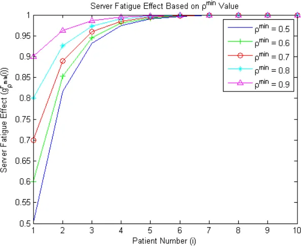
Figure 3.2 Graph of fatigue effect, gFρmin(i), for specified ρmin value. . . 16
Figure 3.3 Graph offρmin(j) for specifiedρminvalue as a function of waiting patients,j. 19
Figure 4.1 Graph of Patient Allotted Times, in hours, with Learning Effect,ρmin= 0.9 36 Figure 4.2 Graph of Patient Allotted Times, in hours, with Learning Effect,ρmin= 0.8 36 Figure 4.3 Graph of Patient Allotted Times, in hours, with Learning Effect,ρmin= 0.7 37 Figure 4.4 Graph of Patient Allotted Times, in hours, with Learning Effect,ρmin= 0.6 37 Figure 4.5 Graph of Patient Allotted Times, in hours, with Learning Effect,ρmin= 0.5 38 Figure 4.6 Graph of Patient Allotted Times, in hours, with Learning Effect,ρmin= 0.55 39 Figure 4.7 Graph of Patient Allotted Times, in hours, with Fatigue Effect, ρmin= 0.9 39 Figure 4.8 Graph of Patient Allotted Times, in hours, with Fatigue Effect, ρmin= 0.8 40 Figure 4.9 Graph of Patient Allotted Times, in hours, with Fatigue Effect, ρmin= 0.7 40 Figure 4.10 Graph of Patient Allotted Times, in hours, with Fatigue Effect,ρmin= 0.6 41 Figure 4.11 Graph of Patient Allotted Times, in hours, with Fatigue Effect,ρmin= 0.5 41 Figure 4.12 Graph of Patient Allotted Times, in hours, with Congestion Effect,ρmin =
0.9 . . . 42 Figure 4.13 Graph of Patient Allotted Times, in hours, with Congestion Effect,ρmin =
0.8 . . . 43 Figure 4.14 Graph of Patient Allotted Times, in hours, with Congestion Effect,ρmin =
0.7 . . . 43 Figure 4.15 Graph of Patient Allotted Times, in hours, with Congestion Effect,ρmin =
0.6 . . . 44 Figure 4.16 Graph of Patient Allotted Times, in hours, with Congestion Effect,ρmin =
Chapter 1
Introduction
Health care expenditures in 2009 were 17.6% of the United State’s gross domestic product, with expenditures related to physician and clinical services, and hospitals growing 4.0% and 5.1%, respectively that same year[5]. It is predicted that national health expenditures will continue to grow 6.1% each year over the next 7 years. Given that a large proportion of the population is reaching retirement age, and will begin to have greater demand for health services, a large amount of pressure is placed on the health care industry to minimize costs. One facet to cutting health care spending is increased efficiency. Appointment scheduling systems provide a means to better match patient demand with health service provider supply. Improvements may lower the cost of care by increasing the number of patients that can be served and increasing utilization of expensive resources. Improvements to appointment scheduling can also lower waiting times, resulting in a better service experience for patients.
When dealing with appointment systems in a health care setting two main groups are in-volved: patients and health care providers. From a patient perspective, as waiting times increase there can be several resulting negative effects. Patients may become frustrated and leave before their appointment time, or may choose to find a new provider in the future. In both situations a loss in revenue for the health care provider may occur. Another aspect that may lead to neg-ative effects for health care providers is the occurrence of idle time for the health care providers between appointments. Although the provider may not be working with a patient they are still being compensated for their time. Additionally, poor scheduling may lead to overtime in order to finish all scheduled appointments, thus resulting in additional cost to the provider.
ap-pointments has prompted a large amount of research. Previous research has focused on queuing methods, the use of simulation models to test various scheduling rules, and optimization mod-els. Standard models consider the arrival of patients to a single stochastic server. The previous use of queuing allows for easier computation and thus more complex models, however the mod-els cannot account for unpredictability. The more recent focus on stochastic modmod-els accounts for every day randomness although adding complexity to the models proves to be more difficult.
Numerous extensions of appointment scheduling models have been explored. For example, some models consider the added probability that a patient may not attend their appointment (no show), or there may only be a finite amount of waiting space for patients. The majority of extensions of this type have focused on the patient behavior. On the other hand, little research has been done on the development of appointment scheduling models that account for server behavior.
In this thesis we focus on provider behavior and how it may affect appointment scheduling. We propose three models which examine the effect of three different behaviors: learning, fatigue, and congestion response. The three behaviors were selected because of their relevance to the health care setting. For example, a learning curve may exist if the longer a health care provider is working, the shorter each appointment may become, because the provider becomes more efficient at the required processes. Alternatively, the longer a provider works, the longer each appointment may become because they are affected by fatigue as the day continues. Finally, in the third model we assume the more patients a provider sees waiting for their appointment the faster the provider performs the service. These server behaviors are observed in many ser-vice systems. Goodale and Tunc[6] examined server behavior affected by learning curves, while Courtois and Georges[2], Gupta[7], Harris[8], and Posner[12] all created models that determine service time based on the current state of customers in the system.
In the models we propose, the learning and fatigue effects were considered to be similar in nature. In each case the service rate was modeled as changing based on the number of patients that had arrived for their appointment. The learning effect produced shorter mean service time with each successive patient, and the fatigue a longer mean service time. The congestion effect was modeled with a different approach, being determined by how many patients were currently waiting for their appointment. In the model we propose, the more patients that are waiting for their appointment the shorter the current patient’s mean service time.
of congestion is modeled through a two stage mixed integer program (2-SMIP). Each of the models are examined for their relevance to producing more effective schedules, and various sensitivities are also examined. Heuristics for scheduling are also produced based on the three server behavior models. These heuristics may produce accurate schedules without the use of complicated models, therefore creating a fast cost effective method for scheduling.
Chapter 2
Literature Review
2.1
Introduction
The scheduling of patient appointments in a health care setting, for example a primary care office or hospital operating room, is a difficult task that requires several different considerations. There are a variety of factors that can influence how quickly a patient is seen by a physician or how long a procedure or consultation may last. One factor that affects patient appointment scheduling is that in many environments, such as outpatient settings, patients are only available at or following their scheduled appointment time. If the health care provider (e.g. physician, operating room) is prepared for the patient prior to their scheduled appointment time, then there is an incurred idling time for the health care server until the patient arrives for their appointment. Thus when scheduling patients for the server’s benefit, it is more advantageous to have patients arrive earlier in order to reduce idling time for the health care provider. However, consideration of the potential for increased patient waiting time must be balanced with the cost of health care provider idle time.
Over the past few decades there has been a large amount of research dedicated to effective methods for scheduling. In this literature review we will discuss some of the most common models and methods. The scheduling methods discussed in this literature review are not all directed at a health care setting, but they are applicable to many contexts. Since the work in this thesis is motivated by problems that arise in a health care context the termscustomerand
2.2
Appointment Scheduling
There have been several studies of models that seek to more effectively schedule appointments for medical environments. In one study done by Ho and Lau[10], the authors examined the application of various appointment scheduling rules for creating a schedule in an outpatient en-vironment. The authors evaluated each of the rule’s ability to decrease waiting time and server idle time. Some of the rules examined were variations on a previous set of work by Welch and Bailey [14]. These rules focused on the arrival time, ai, for each patient i and which patients
would haveai= 0 and how the remaining patient arrival times were determined. For example,
one rule sets a1 = a2 = 0 and for i > 2, ai = ai−1 +µ where µ is the mean service rate. Another rule assigns a1 = 0, a2 = 0.3, a3 = 0.6, a4 = 0.9, and for i > 4, ai = ai−1 +µ. The scheduling rules, or heuristics, were tested using a Monte Carlo simulation. Through their work Ho and Lau found that an effective scheduling rule could be identified only when three main environmental factors were known. These factors were the probability of patients being a no show, the coefficient of variation of service time, and the total number of patients to be scheduled. Additionally, Ho and Lau suggested that the ratio of cost for patient wait time to provider idle time is an important factor to consider.
Another approach to appointment scheduling that has been taken, is based on optimization models in which the objective is to minimize costs associated with expected patient waiting and server idling. Weiss[13] examined two different aspects of this type of model: assigning patient arrival times based on a given schedule, and designing a sequence of arrivals for a given set of patients. He studies the problem in the context of scheduling procedures in an operating room. Weiss approaches the problem by showing that the problem resembles that of the well-known newsvendor model. Given a set ofn procedures which are already placed in order, each procedure has an associated set of characteristics:
zi: random processing time forith procedure
li: completion time of ith procedure
ai: estimated start (arrival) time ofith procedure
pi: actual start time of ith procedure
li−1≤ai ⇒pi =ai (2.1)
where ifli−1 is strictly less thanai then this would result in idle time for the health care staff.
Conversely if i−1 ends on time or later then:
li−1 ≥ai ⇒pi=li−1 (2.2)
and ifli−1 is strictly greater thanai then this results in a waiting time for both theith patient
and their associated staff. In Weiss’ model the total wait (wi) and idle (si) time, respectively,
can be represented as:
wi = max(0, pi−ai) = max(0, li−1−ai) (2.3)
si = max(0, ai−li−1). (2.4)
The objective is to minimize the total expected cost, which can be represented as:
E(cost) =E X
i
cwwi+
X
i
cssi
!
. (2.5)
Here cw and cs represent the cost of wait and idle time, respectively.
In Equation (2.5) the cost associated with idle time is analogous to the surplus cost in the newsvendor model, since idling indicates that the actual demand for server time was less than the server’s actual time supply. The cost of waiting corresponds to the newsvendor’s cost of a shortage, because waiting occurs when the actual demand for server time is greater than the actual supply of time.
Another study on appointment scheduling by Bosch and Dietz[1] views the appointment scheduling problem as a first-come first-serve queuing system. In this model they follow the same premise as previously mentioned models, where they seek to minimize the cost of cus-tomer waiting time and server overtime by assigning cuscus-tomer arrivals. However, there are two additional considerations, the probability of customer no shows and the requirement to evenly space customer arrivals. As with previous models Bosch and Dietz[1] determine a customer’s service time by considering it to be a random variable from a chosen positive distribution. However, another probability is also associated with customers, their potential to fail to show for an appointment. The central goal of this model is to find a set of customer arrival times that must occur at evenly spaced intervals.
A different approach to appointment scheduling, taken by Murray and Berwick[11] intro-duces the concept of advanced access appointment scheduling. They examine a scheduling strategy which allows patients to request an appointment same day, rather than call and make an appointment for another day in the future. Murray and Berwick argue that this form of ap-pointment scheduling would allow medical offices to fulfill daily demand as it arrives rather than postpone the demand until a future date. Theoretically this process would decrease the factors that increase patient and staff idle time. These factors include: time spent by the medical staff booking and reminding patients of their appointments and a patient’s probability of skipping the appointment. Murray and Berwick assert that the predicted advantage of advanced access care depends on three general designs. First, advanced access aims to reduce the gap between when demand first appears and when it is satisfied. Then second, the reduction between de-mand and supply would additionally lead to a reduced patient dede-mand since the physician has become more accessible. Third the authors suggest, these changes would lead to an increase in the supply of physician appointments on a daily basis, and would thus more effectively handle a sudden increase in demand. However, such a scheduling policy has the limitation of increasing physician idle time, i.e., unused appointment slots.
A more recent generalization of Weiss’ optimization model was proposed by Denton and Gupta[3]. They examined the scheduling of n patients when a patient’s appointment dura-tion is uncertain. Denton and Gupta proposed a two stage stochastic linear program (2-SLP) that seeks to minimize the expected cost of patient waiting time, server idle time, and sys-tem overtime. They refer to this model as the appointment scheduling problem (ASP). Their model serves as a basis for the models studied in this thesis. Thus, we describe it in detail below.
in-volves a set ofnjobs, where patients are assumed to always arrive on time to their appointment. The first stage decision variables are denoted by:
x: vector of job allowances for first n−1 jobs The second stage decision variables are:
w: vector of wait times associated with xand Z s: vector of server idle times associated withxand Z
o: system overtime associated with given set of jobs g: earliness for a given sequence of jobs
The model parameters include:
Z: vector of random job durations
d: day length, total allotted time for job sequence cw: vector of cost coefficients for customer waiting time cs: vector of cost coefficients for server idle time
co: cost coefficient for server overtime
Note that we use bold font to denote vectors and upper case to denote random variables.
The ASP has the following objective function:
minEZ
( n
X
i=2
cwi wi+ n
X
i=2
csisi+coo
)
(2.6)
The expectation in (2.6) is with respect to a probability distribution defined by a finite set of scenarios. A scenario, ωk, is a single set of realizations of job durations wherekis the index of
a set of K scenarios. Each scenario, k, has probability pk of occurring. The objective function can be expressed as:
min K X k=1 pk n X i=2
cwi wik+
n
X
i=2
csiski +cook
!
(2.7)
The constraints in the ASP follow the logical argument that the difference between the actual duration of a patient’s appointment (Zi) and their estimated time allowance (xi) must
be equal to the difference between the following patient’s waiting time (wi+1) and the current patient’s waiting time (wi), minus the server idle time that occurs between patientiand i+ 1,
(si+1). This must be true for each patienti, given thatw1 ands1 are zero since the first patient
arrives on time at time zero, creating n−1 decision variables. Therefore the given objective function, (2.7), is subject to the following constraints:
w2k−sk2 =Z1k−x1 −w2k+w3k−sk3 =Z2k−x2
· · · ·
−wnk−1+wkn−skn=Znk−1−xn−1
xi≥0∀ i, wik, ski ≥0 ∀(i, k) (2.8)
The final constraint placed on the model restricts the calculation of overtime and earliness:
−wnk+ok−gk=Znk−d+
n−1
X
j=1
xj (2.9)
Denton and Gupta studied results based on this model to draw insights about optimal appoint-ment schedules. This model forms the basis for the extensions discussed in Chapters 3 and 4.
2.3
Server Behavior
types of server behaviors that could affect appointment scheduling, and some of the literature supporting the selection of these behaviors.
2.3.1 Learning and Fatigue
One environmental factor that could have an effect on servers is related to changes during progression of the day. Two potential effects that may result in this are: learning and fatigue. A learning effect may be present when the server decreases the mean service time as the day continues. Conversely, a server may also be affected by fatigue and increase their mean service time as the day progresses.
Goodale and Tunc[6] produced a mixed integer program that includes service rates that are affected by a server’s learning curve. When modeling the effect of a learning curve, their model used two sets of servers. One set of servers known as thecore employeesmaintained a constant service rate, and the other set, the contingent employees, had varying service rates that were affected by learning or fatigue. Once an optimal schedule was produced by the model the costs associated with each of the employee sets were compared to see if there was an advantage to considering service time variations.
The learning curve employed by Goodale and Tunc was modeled through the following exponential equation:
f·n−b µave
(2.10)
wheref is the initial service time forcontingent employees,nis the number of customers served bycontingent employees,bis the learning parameter, andµave is the average service rate of the
employee population. Examining the equation reveals that as the number of customers served by acontingent employeeincreases the fraction, (2.10), also becomes smaller meaning a decrease in service time.
The Goodale and Tunc model uses values that are constant or part of a distribution, and fails to consider how different a set of appointments may be from day to day. Two of the ap-pointment scheduling models produced in this thesis focus on the server behaviors of learning and fatigue and utilize a stochastic model. Our learning and fatigue server behavior models have random service times that more accurately represent appointment schedules in a physi-cians office.
2.3.2 Congestion
In this section we discuss how waiting room congestion may affect the amount of time that each patient should be allotted for their appointments. A common observation for many service systems is that as a queue for a service grows, the server increases its pace. Some studies suggest this theory can be incorporated into models.
Some studies have attempted to measure the effect of the queue on the server’s pace in practice. In a study by Deveugele, et al.[4] a group of physicians and their patients were ob-served to determine what factors determine the length of a consultation. They found that a negative correlation existed between the physician’s workload and the patient’s consultation lengths. Another study on a collection of physicians and their patients done by Heaney, et al. [9] had similar results. They also found a negative relationship between queue size and consul-tation length, and additionally discovered a similar negative relationship between a patient’s placement in the queue and their consultation length.
An article by Gupta[7] considers a queuing system that uses the current state of the system to determine particular distributions. The queuing model produced by Gupta is defined by an input which is hyper-Poisson with an assigned mean arrival rate, a first-come first-served service policy, and an exponential service time distribution. Gupta’s model assigns the arrival and service time mean rates to be state dependent. Therefore, the mean arrival and service time rates change based on arbitrary functions relating the rates to the current state of the system. Gupta also assumes that there is a finite number of patients that can be in the system at any time. The finite consideration not only adds a more realistic aspect to the system but also allows Gupta to obtain solutions for their model.
Another model considering environmental effects was proposed by Harris[8]. Harris’ takes an M/G/1 queuing system and treats each customer’s service time as a stochastic process that is classified by the total number of customers that are in the queue at the time a customer begins service. Each customer’s service time is created by determining the number of customers in the queue at the time each customer begins their service. The number of customers, i, at the be-ginning of service is then used to find the variable,Mi, which is part of a predetermined group.
The determinedMi is then used to create the service time,Ti, for each customer. Harris
exam-ines three different queuing models: one that has state independent service times, the second that considers an independent service time distribution for customer 1 and a state dependent distribution for customers 2 through n, and a third that has a state dependent service time distribution for all n customers. Harris determined that the use of state dependent processes requires different solving methods, and that most future research would be centered around finding these methods.
2.4
Contributions of this Thesis
Chapter 3
Appointment Scheduling in the
Presence of Varying Server Behavior
3.1
Introduction
Adjusting an appointment scheduling model to appropriately account for changes in the server’s behavior over time may improve appointment schedules by reducing expected waiting and/or idle time. Failing to account for changes, on the other hand, could lead to a schedule that over or underestimates the duration of each patient’s appointment. The server behaviors we focus on in this Chapter are: learning, fatigue, and congestion response. In this section we intend to produce our own models that will account for these selected server behaviors.
We propose two 2-SLP models that include the server behaviors of learning and fatigue and one 2-SMIP that includes server behavior affected by congestion. The models are extensions to the ASP model proposed by Denton and Gupta [3]. We explain the assumptions associated with each of the models, and we provide a detailed description of the stochastic programming formulation.
3.2
Model Formulations
We extend the model by Denton and Gupta[3] to include the influence of the three types of server behavior discussed in Chapter 2: learning, fatigue, and congestion. The formulation of the first two server behaviors, learning and fatigue, will be provided first followed by the formulation of the congestion model.
3.2.1 Learning and Fatigue Formulation
In our model we represent the effects of learning and fatigue as a change in the proportion of each customer’s service time. We use the following equations to represent the effects of learning and fatigue, respectively:
gLρmin(i) = (1−ρmin)e(1−i)+ρmin (3.1)
gFρmin(i) = (ρmin−1)e(1−i)+ 1 (3.2)
In each equation ρmin represents the selected server behavior minimum effect value for learning (L) and fatigue (F), and i is and index denoting the position of the patient in the appointment sequence. The functions in equations (3.1) and (3.2) are multiplied with service time in each of their respective models. Thus, each behavior effect equation produces the effect of scaling each customer’s random service time. A better understanding of the two equations can be gained by looking at Figures 3.1 and 3.2 which show a graph of the value of each equation by patient number for a set of n= 10 patients, and several differentρmin values. In Figure 3.1 the server learning effect is decreasing, resulting in a decrease in the mean service time, with respect to the patient index. Figure 3.2 shows the server fatigue effect increasing with each additional patient which will result in an increase in the mean service time with respect to patient index.
The extended models for learning and fatigue are created by simply multiplying the respec-tive server behavior equations with the actual job duration time,Zi. In the case of the learning
formulation, the objective remains the same as Equation 2.6 in the ASP model,
minE
( n
X
i=2
cwi wi+ n
X
i=2
csisi+coo
)
Figure 3.1: Graph of learning curve effect,gLρmin(i), for specified ρmin value.
and is now subject to a new set of constraints:
w2−s2 =Z1·gρLmin(1)−x1 −w2+w3−s3 =Z2·gρLmin(2)−x2
· · · ·
−wn−1+wn−sn=Zn−1·gρLmin(n−1)−xn−1
xi≥0, wi≥0, si≥0∀ i= 1, . . . , n (3.4)
The fatigue formulation is very similar, differing only in the server behavior parameter that is used.
minE
( n
X
i=2
cwi wi+ n
X
i=2
csisi+coo
)
(3.5)
w2−s2 =Z1·gρFmin(1)−x1 −w2+w3−s3 =Z2·gρFmin(2)−x2
· · · ·
−wn−1+wn−sn=Zn−1·gρFmin(n−1)−xn−1
xi≥0, wi≥0, si≥0∀ i= 1, . . . , n (3.6)
3.2.2 Congestion Formulation
they arrived. Following is a detailed mathematical formulation of this model.
The following indices were used in the model: i: index for patients
j: index for server queue size (number of patients waiting)
ω: index for scenarios
In addition, the following notation, coupled with the indices listed above, defines the model parameters.
n: number of routine patients
cw: cost vector associated with patient waiting time co: overtime cost coefficient with respect tod d: planned length of clinic day
fρmin(j): function determining congestion effect produced by j patients waiting and selected
ρmin parameter
ρmin: minimum congestion parameter
z(ω): vector of random job durations for patients
ξ(ω): random vector containing second stage scenario dependent parameters, ξ(ω) ={z1(ω), ..., zn(ω)} wheren is the number of patients,z ∈Rn.
The cost vectors cw and co can be adjusted accordingly for each job, depending on how cost is affected by a particular customer or server. The congestion effect fρmin(j) is a function of
the number of patients that are currently waiting in the queue and a previously specified value of ρmin. The function produces a scalar value that is used to find the fraction of the original time the server will take to service a particular patient. In this thesis we use a linear model for congestion, the applied numerical values for five differentρmin values are displayed in Table 3.1. Additionally a graphical display of each of the five functions is shown in Figure 3.3
The vector z(ω), which varies according to scenario, has probability distribution P ∈ Rn
Table 3.1: Linear congestion effect values as a function of the number of patients waiting for ρmin = 0.5, 0.6, 0.7, 0.8, 0.9, 1.0.
j 1 2 3 4 5 6 7 8 9 10
f1(j) 1.0 1.0 1.0 1.0 1.0 1.0 1.0 1.0 1.0 1.0
f0.9(j) 1.0 0.989 0.978 0.967 0.956 0.944 0.933 0.922 0.911 0.9 f0.8(j) 1.0 0.978 0.956 0.933 0.911 0.889 0.867 0.844 0.822 0.8 f0.7(j) 1.0 0.967 0.933 0.9 0.867 0.833 0.8 0.767 0.733 0.7 f0.6(j) 1.0 0.956 0.911 0.867 0.822 0.778 0.733 0.689 0.644 0.6 f0.5(j) 1.0 0.944 0.889 0.833 0.778 0.722 0.667 0.611 0.556 0.5
xi: time allotted for patienti
ai: decision variable defining the time when patientiarrives
uii0: binary decision variable defining the arrival sequence of patients (1 if i0 arrives after i arrives, 0 otherwise)
The second stage decision variables are:
li(ω): decision variable defining the time when patient ileaves
pi(ω): decision variable defining the time when patientibegins their procedure
vii0(ω): binary decision variable defining which patients arrive before patient i0 begins their procedure (1 ifi0 is arrives before ibegins their procedure, 0 otherwise)
qii0(ω): binary decision variable defining which patients are waiting when patienti0begins their procedure (1 ifi0 is waiting when ibegins their procedure, 0 otherwise)
ri(ω): integer decision variable defining the number of patients waiting when i begins their
procedure
tij(ω): binary decision variable defining the number of patients waiting when i begins their
procedure (1 ifj patients are waiting, 0 otherwise) ˆ
zi(ω): decision variable defining the procedure duration for patient i where congestion is
in-cluded
wi(ω): waiting time for patienti
si(ω): idling time associated with patienti
o(ω): overtime with respect to the length of clinic dayd
The objective function that is to be minimized in the second stage, given scenario ω, is:
Q(x,ξ(ω)) = min
n
X
i=1
cwwi(ω) +coo(ω). (3.7)
minQ(x) (3.8a) s.t.
ai= i−1
X
k=1
xk ∀(i, ω) (3.8b)
ai0 −ai−M uii0 ≤0 ∀(i, i0) (3.8c)
xi, ai≥0, uii0 ∈ {0,1} (3.8d)
where
Q(x) =Eω[Q(x,ξ(ω))]. (3.9)
The first stage problem is then combined with the second stage problem to obtain the complete formulation, which is:
minEω
" n X
i=1
cwwi(ω) +coo(ω)
#
s.t.
li(ω)−wi(ω)−zˆi(ω) = i−1
X
k=1
xk ∀(i >1, ω) (3.10b)
l1(ω)−z1(ω) = 0ˆ ∀(ω) (3.10c)
pi(ω)−ai−wi(ω) = 0 ∀(i, ω) (3.10d)
pi(ω)−ai0−M vii0(ω)≤0 ∀(i, i0, ω) (3.10e) 2qii0(ω)−uii0 −vii0(ω)≤0 ∀(i, i0, ω) (3.10f)
ri(ω)− i
X
i0=1
qii0(ω) = 0 ∀(i, ω) (3.10g)
ri(ω)− n−1
X
j=0
jtij(ω) = 0 ∀(i, ω) (3.10h)
n−1
X
j=0
tij(ω) = 1 ∀(i, ω) (3.10i)
ˆ zi−
n−1
X
j=0
fρmin(j)tij(ω)zi(ω) = 0 ∀(i, ω) (3.10j)
wi(ω)−si(ω)−wi−1(ω)−zˆi−1(ω) =−xi−1 ∀(i >1, ω) (3.10k)
w1(ω) = 0 ∀(ω) (3.10l)
n
X
i=1
(ˆzi(ω) +si(ω))−o(ω)≤d ∀(ω) (3.10m)
li(ω), pi(ω),zˆi(ω), wi(ω), si(ω), o(ω)≥0 ∀(i, ω) (3.10n)
qii0(ω), vii0(ω), tij(ω)∈ {0,1} ∀(i, i0, j, ω) (3.10o)
ri(ω)∈Z+ ∀(i, ω). (3.10p)
The constraints (3.8b), (3.8c), and (3.10e)-(3.10j) are what define the congestion response of the server. The constraints are broken into two groups for description, (3.8c),(3.10e), and (3.10f), and (3.10g)-(3.10j). The constraints (3.8c), (3.10e), and (3.10f) determine values that are necessary to be known to apply a congestion effect to this model. Constraint (3.8c),
ai0 −ai−M uii0 ≤0 ∀(i, i0, ω),
is a first stage constraint defined by first stage decision variables ai and uii0. This constraint determines which patients arrive after patient i. When uii0 = 0 the remaining portion of the equation must be less than or equal to zero, and since the arrival times for patient i and i0, where i6= i0, cannot be the same this means it must be less than zero. Therefore, the arrival time for patient i,ai, must be a larger value or later time than the arrival time for patient i0,
ai0. Conversely, when uii0 = 1, since it is multiplied by some sufficiently large number M, this causes the left side of the equation to be a large negative number, allowingai0 to be later than ai. Constraint (3.10e),
pi(ω)−ai0 −M vii0(ω)≤0∀(i, i0, ω),
determines which patients arrive before patientibegins their procedure. When vii0(ω) = 0 the remaining portion of the equation must be less than or equal to zero. Therefore, the arrival time for patient i0 must be equal to, or later than, the procedure start time for patient i, pi,
and this would be consistent with vii0(ω) = 0. When vii0(ω) = 1, since it is multiplied by some sufficiently large number, M, this removes the restrictions on the rest of the equation allowing ai0 to occur beforepi. Constraint (3.10f),
2qii0(ω)−uii0−vii0(ω)≤0 ∀(i, i0, ω),
consistent with patient i0 waiting when patienti begins their procedure, or qii0(ω) = 1. Addi-tionally, when qii0(ω) = 0 the restrictions are released from the remaining variables, allowing patient i0 to not be waiting when patient ibegins their procedure.
The next group of constraints discussed are (3.10g)-(3.10i). The first two constraints (3.10g) and (3.10h):
ri(ω)− i
X
i0=1
qii0(ω) = 0 ∀(i, ω)
ri(ω)− n−1
X
j=0
jtij(ω) = 0 ∀(i, ω)
both assign the value for the number of patients waiting when patientibegins their procedure. Constraint (3.10g) requires thatri(ω) is equal to the sum over the binary variableqii0(ω). Con-straint (3.10h) requires thatri(ω) is equal to the binary variabletij(ω), determining whetherj
patients are waiting when patientibegins their procedure times thosejpatients. The constraint (3.10i),
n−1
X
j=0
tij(ω) = 1 ∀(i, ω)
simply assures that there can only be one value, j, of patients waiting when patient i begins their procedure.
These two groups of constraints, (3.8c), (3.10e), and (3.10f), and (3.10g)-(3.10i), determine the congestion effect to be applied, which is defined by constraint (3.10j),
ˆ zi−
n−1
X
j=0
fρmin(j)tij(ω)zi(ω) = 0 ∀(i, ω).
ˆ
zi, must be equal to the summation over the potential number of patientsj, however since the
binary variabletij is a product in this summation only one value for patient iwith j patients
waiting not equal to zero may be found. Therefore, the congestion effect for patient i will be equal to the product of the congestion effect for j patients waiting and the job duration for patient i, zi(ω). The congestion effect function, fρmin(j), will be defined by several different
functions in the next chapter. The values are fractional to represent the portion of the previous procedure duration that will be used.
Chapter 4
Numerical Results
4.1
Introduction
A series of numerical experiments were performed to evaluate the three models described in Chapter 3. The results presented in this Chapter include an evaluation of the structure of the optimal schedule, a sensitivity analysis of the models with respect to input parameters, and a set of three heuristics based on each of the server behavior models. Through this analysis we seek to determine if the models are able to produce significantly more cost effective schedules than standard models that ignore server behavior. We further hope to understand which vari-ables have the most effect on cost, and should therefore be considered in the future.
The models were solved using OPL-CPLEX 12.2. The solutions, on average took from thirty to fifty seconds to be returned on a computer with a 2.83 GHz IntelCoreTM2 Quad Processor and 8 GB RAM.
4.2
Methodology
The models were programmed using OPL-CPLEX. The following settings were used throughout Chapter 4 unless noted otherwise: n= 10, cw = 1, co = 1, cs = 0,d= 4, z(ω) ∼U(0,1). The determination of the learning (gρLmin), fatigue (gFρmin), and congestion (fρmin) effect functions,
on the mean and 95% confidence intervals which were computed using 30 independent model runs. Similarly in Section 4.6 an analysis is performed on the allotted time for each patient and again thirty model runs were used to compute the mean and 95% confidence interval for the analysis.
4.3
Model Validation
The validity of each model was determined through comparison to the ASP model proposed by Denton and Gupta[3] (which we refer to as the ASP model in the remainder of this Chapter). We assumed that because the ASP model was previously validated we could verify our models by showing that each model is equivalent to the ASP model. Each of the three behavior models were validated by reducing each model back to the ASP model. Then the same set of values were run through each reduced server behavior model and the ASP model, and then each model was compared back to the base ASP model to conclude that identical solutions were being produced.
In the case of the learning and fatigue server behavior models their similarity with the ASP model allowed for easy verification. Each of the two behavior models were reduced by restricting their respective effect functions to be equal to 1, thus resulting in no effect from learning and fatigue. Then equivalent values for job duration were run through each of the behavior models and the base ASP model while the same cost for overtime, waiting, and idle time were used along with 10 patients and scenarios, and equal clinic day length. Identical solutions were pro-duced for optimal objective value and allotted time between each behavior model and the ASP model, indicating that the learning and fatigue models are only a variation on the previously validated ASP model.
4.4
Server Effect on Total Cost of the System
The first set of experiments that was run on each of the models sought to determine if failing to account for server behavior has a significant effect on the total cost of the system. In order to conduct this experiment the results from the three server behavior models were compared to the ASP model that does not account for server behavior. The effect of ignoring server behavior when it is present was modeled by manipulating each of the server behavior models such that their solutions were no longer accounting for their respective server behavior, but the service times were still being altered by the server behavior. The resulting server behavior models were then used to determine the allotted time for each patient (appointment schedule) and the mean optimal objective value (total cost) associated with each of these sets of allotted times, then this data was examined to determine if there was an associated loss in profit or time.
The first step of the experiment was conducted by finding and recording the mean opti-mal objective values corresponding to applying each of the three server behavior models, and then comparing these results to the standard model. Each model uses a server effect function (gρLmin(i), gρFmin(i), fρmin(j)) that is determined by an initially selected value ofρmin and either
the current patient number (learning and fatigue models) or the current number of waiting patients (congestion model). The experiment was run on each model withn= 10 patients and ρmin = 0.5,0.6,0.7,0.8,0.9. The mean optimal objective function values were recorded for each server behavior model and compared to the standard model.
The second step requires creating a model for each server behavior that does not account for the respective server behavior when producing a schedule. Settingρmin= 1.0 for each model results in no server behavior effect. Therefore each model, the 2-SLP learning and fatigue, and the 2-SMIP congestion model were run setting ρmin = 1.0 and the produced set of allotted times,xi, for each patient was recorded. The program was then run again for each model and
their corresponding effect function, withρmin = 0.9,0.8,0.7,0.6,0.5; however, the allotted times were held to be equal to those previously recorded for the ρmin = 1.0. Restriction of the time allowance values in this way simulates the effect of using a model that does not account for server behavior to produce a schedule in a situation where server behavior alters patient service times.
Table 4.1: Comparison of objective values when a learning effect is present and time allowance values do account for a learning effect and when the learning effect is ignored. ∗ indicates statistically significant difference between means.
Optimal Objective Value Optimal Objective Value Ignoring Learning
Mean 95% CI Mean 95% CI
gL1(i) 8781.44 (8662.21, 8900.68) -
-g0L.9(i) 6521.35 (6443.09, 6599.61) 6031.39 (5281.96, 6780.81) g0L.8(i) 4288.64 (4235.86, 4341.41) 4208.216 (3684.53, 4731.90) g0L.7(i) 2469.28 (2441.26, 2497.30) 2791.14 (2443.785, 3138.49) g0L.6(i) 1165.82∗ (1143.59, 1188.04) 1893.42∗ (1658.62, 2128.21) g0L.5(i) 456.45∗ (448.28, 464.61) 1304.08∗ (1142.23, 1465.93)
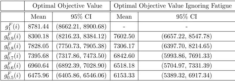
Table 4.2: Comparison of objective values when a fatigue effect is present and time allowance values do account for a fatigue effect and when the fatigue effect is ignored.
Optimal Objective Value Optimal Objective Value Ignoring Fatigue
Mean 95% CI Mean 95% CI
g1F(i) 8781.44 (8662.21, 8900.68) -
-g0F.9(i) 8300.18 (8216.23, 8384.12) 7602.50 (6657.22, 8547.78) g0F.8(i) 7828.05 (7750.73, 7905.38) 7306.17 (6397.70, 8214.65) g0F.7(i) 7395.68 (7317.86, 7473.50) 6842.60 (5993.86, 7691.33) g0F.6(i) 6960.64 (6892.39, 7028.90) 6518.18 (5704.97, 7331.39) g0F.5(i) 6475.96 (6405.86, 6546.06) 6153.33 (5389.32, 6917.34)
Table 4.3: Comparison of objective values when a congestion effect is present and time al-lowance values do not account for congestion and when congestion is ignored. ∗ indicates sta-tistically significant difference between means.
Optimal Objective Value Optimal Objective Value Ignoring Congestion
Mean 95% CI Mean 95% CI
f1(j) 9011.72 9011.72 -
-f0.9(j) 7193.90 (7118.42, 7269.37) 7220.61 (7144.46, 7296.77)
f0.8(j) 5635.54 (5574.27, 5696.81) 5721.61 (5664.73, 5778.49)
f0.7(j) 4067.90∗ (4014.83, 4120.98) 4320.13∗ (4262.99, 4377.28)
f0.6(j) 2718.07∗ (2674.98, 2761.17) 3167.03∗ (3134.69, 3199.19)
in the mean optimal objective value are only seen when the learning effect on service time is significant.
The results for the fatigue model, in Table 4.2, do not show the same effect as the learning model. There is a decrease between mean costs when fatigue is accounted for and when it is not. Comparing the 95% confidence intervals, however, does not show a significant decrease, indicating that failing to account for fatigue in appointment scheduling may not lead to a sig-nificant difference for the specific test cases we explored. We believe that one main reason why no significant difference was found for the fatigue model is due to the fatigue effect function, Equation 3.2. The fatigue effect function, the graph of which can be seen in Figure 3.2, is an increasing exponential function with an upper bound of 1. The speed at which the function increases to 1 causes, for the majority of patients, the fatigue effect to be fairly minimal (i.e. the fatigue effect is generally≥0.9). Therefore, the majority of service times are only minimally altered by fatigue and it is not surprising that there is no significant difference in the mean optimal objective value.
The results for the congestion model are shown in Table 4.3. Table 4.3 shows an increase in mean optimal objective value between when congestion is considered in the appointment scheduling model and when congestion is ignored. The comparison of the confidence intervals also reveals statistically significant differences, as indicated by the∗. In the case of the conges-tion coefficient funcconges-tion with theρmin values 0.8 and 0.9 the confidence intervals overlap, which would indicate that there is no significant difference in cost between when congestion is con-sidered and when it is not concon-sidered. However, for ρmin ≤0.7 the differences are statistically
significant. This difference indicates that failing to consider congestion when it has an effect on the system may lead to increased costs that could be avoided.
4.5
Sensitivity Analysis
The second set of experiments performed on each of the server behavior models investigates the sensitivity of each model to α, where α= ccwo. This measures the effect of varying ratios of
mean optimal objective value, for each associatedα andρmin value were recorded. The results for the learning server behavior model are shown in Tables 4.4, 4.5, and 4.6, then the fatigue model results are displayed in Tables 4.7, 4.8, and 4.9. Finally the sensitivity of changes in cost of waiting and overtime for the congestion behavior model are shown in Tables 4.10, 4.11, and 4.12. There is a table for all three server behavior models whenα= 1 (4.4, 4.7, 4.10), meaning cw andco are both equal, this table serves as a comparison to the tables for each server behavior model when co and cw are separately increased. The tables when α = 1 help us to determine the effect on the mean optimal objective value whencw and co are increased.
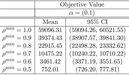
Each Table of different α values for the learning server behavior effect show a significant increase in the mean optimal objective value as ρmin increases. Table 4.4 when compared to Tables 4.5 and 4.6 shows a significant increase in the mean optimal objective value with respect toρmin whencwandcoare increased, except forρmin = 0.5 in Table 4.5. The significantly lower mean optimal objective value forα= 1 compared toα= 0.1 andα= 10 follows intuitively be-cause of an increase in eitherco orcw. The significant decrease in mean optimal objective value forρmin = 0.5 whenα= 1 compared to whenα= 0.1 we estimate stems from the large decrease in allotted time for patients whenρmin= 0.5. The large decrease in allotted time indicates that any increase in overtime cost has minimal consequence because overtime is very seldom required.
Looking at the effect of increasing eitherco orcw in the learning behavior model. Table 4.5
reveals higher mean optimal objective values compared to Table 4.6 with respect toρmin. Table 4.5 represents whenco is increased. The higher optimal objective values in Table 4.5 imply that increasing only co will lead to higher optimal objective values than when increasing cw only.
These results indicate that the learning server behavior model may be more sensitive to changes in cost of overtime than the cost of waiting.
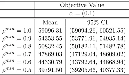
The Tables for each α value for the fatigue server behavior effect again show a significant increase in the mean optimal objective value as ρmin increases. Table 4.7 when compared to Tables 4.8 and 4.9 shows a significant increase in mean optimal objective value with respect to ρmin when the waiting or overtime costs are increased. Again, the significant lower mean optimal objective value for α = 1 compared to α = 0.1 and α = 10 results from the increase inco orcw. The comparison of Tables 4.8 and 4.9 similar to the learning behavior model, show a significant increase in mean optimal objective value with respect to ρmin for Table 4.8. The similar results for the fatigue server behavior model indicate that this model may also be more sensitive to changes in overtime cost.
Table 4.4: Mean and 95% confidence interval on the mean optimal objective value of the server learning behavior model whenα= 1
Objective Value α= (1)
Mean 95% CI
ρmin= 1.0 8935.01 (8872.45, 8997.45) ρmin= 0.9 7193.895 (7118.42, 7269.37) ρmin= 0.8 5635.54 (5574.27, 5696.81) ρmin= 0.7 4004.92 (3920.94, 4088.90) ρmin= 0.6 2747.98 (2654.03, 2841.93) ρmin= 0.5 1638.77 (1595.46, 1682.08)
Table 4.5: Mean and 95% confidence interval on the mean optimal objective value of the server learning behavior model whenα= 0.1
Objective Value α= (0.1)
Mean 95% CI
ρmin= 1.0 59096.31 (59094.26, 60521.55) ρmin= 0.9 39374.43 (38907.57, 39841.30) ρmin= 0.8 22915.45 (22498.28, 23332.62) ρmin= 0.7 10475.22 (10240.22, 10710.22) ρmin= 0.6 3461.42 (3371.19, 3551.65) ρmin= 0.5 752.01 (726.20, 777.81)
Table 4.6: Mean and 95% confidence interval on the mean optimal objective value of the server learning behavior system when α= 10
Objective Value α= (10)
Mean 95% CI
ρmin= 1.0 17498.52 (17496.47, 17654.97) ρmin= 0.9 14296.34 (14170.78, 14421.90) ρmin= 0.8 11255.31 (11156.12, 11354.51) ρmin= 0.7 8288.40 (8212.21, 8364.59) ρmin= 0.6 5105.60 (5056.08, 5155.11)
Table 4.7: Mean and 95% confidence interval on the mean optimal objective value of the server fatigue behavior model whenα= 1
Objective Value α= (1)
Mean 95% CI
ρmin= 1.0 8935.01 (8872.45, 8997.45) ρmin= 0.9 6215.23 (6110.68, 6325.94) ρmin= 0.8 5635.54 (5574.27, 5696.81) ρmin= 0.7 4004.92 (3920.94, 4088.90) ρmin= 0.6 2747.98 (2654.03, 2841.93) ρmin= 0.5 1638.77 (1595.46, 1682.08)
Table 4.8: Mean and 95% confidence interval on the mean optimal objective value of the server fatigue behavior model whenα= 0.1
Objective Value α= (0.1)
Mean 95% CI
ρmin= 1.0 59096.31 (59094.26, 60521.55) ρmin= 0.9 54353.55 (53771.96, 54935.14) ρmin= 0.8 50832.45 (50182.11, 51482.78) ρmin= 0.7 47869.03 (47129.04, 48609.02) ρmin= 0.6 44330.79 (43792.64, 44868.94) ρmin= 0.5 39791.50 (39205.66, 40377.33)
Table 4.9: Mean and 95% confidence interval on the mean optimal objective value of the server fatigue behavior model whenα= 10
Objective Value α= (10)
Mean 95% CI
ρmin= 1.0 17498.52 (17496.47, 17654.97) ρmin= 0.9 17011.29 (16845.58, 17177.00) ρmin= 0.8 16280.14 (16140.99, 16419.29) ρmin= 0.7 15597.57 (15452.08, 15743.07) ρmin= 0.6 15046.39 (14920.50, 15172.28)
found. Tables 4.10, 4.11, and 4.12 show that as the ρmin value increases the mean optimal objective value also increases. Tables 4.11 and 4.12 display the same increased mean optimal objective values for Table 4.11 when co is increased, however these results are only found when
ρmin ≥0.6. Conversely, forρmin = 0.5 Table 4.12 and Table 4.11 return lower and higher mean optimal objective values, respectively. It appears that the congestion model may be more sen-sitive to increases in overtime cost, but sensitivity may also be dependent upon theρmin value.
Table 4.10: Mean and 95% confidence interval on the mean optimal objective value of the server congestion behavior model when α= 1
Objective Value α= (1)
Mean 95% CI
ρmin= 1.0 8935.01 (8872.45, 8997.45) ρmin= 0.9 7193.895 (7118.42, 7269.37) ρmin= 0.8 5635.54 (5574.27, 5696.81) ρmin= 0.7 4004.92 (3920.94, 4088.90) ρmin= 0.6 2747.98 (2654.03, 2841.93) ρmin= 0.5 1638.77 (1595.46, 1682.08)
Table 4.11: Mean and 95% confidence interval on the mean optimal objective value of the server congestion behavior model when α= 0.1
Objective Value α= (0.1)
Mean 95% CI
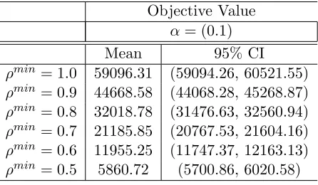
ρmin= 1.0 59096.31 (59094.26, 60521.55) ρmin= 0.9 44668.58 (44068.28, 45268.87) ρmin= 0.8 32018.78 (31476.63, 32560.94) ρmin= 0.7 21185.85 (20767.53, 21604.16) ρmin= 0.6 11955.25 (11747.37, 12163.13) ρmin= 0.5 5860.72 (5700.86, 6020.58)
noted was the positive correlation between optimal objective value and the ρmin value. This positive correlation indicates that as the effect of congestion increases (ρmin decreases), there tend to be lower expected costs of waiting and overtime. The second observation made when comparing increased overtime cost (α = 0.1) and waiting cost (α= 10) shows that the learning, fatigue, and congestion (whenρmin ≥0.7) behavior models are more sensitive to changes in cost of overtime. Then finally it was observed that for the congestion effect function whenρmin = 0.5 there is a higher sensitivity to increases in the cost of waiting time, relative to overtime.
4.6
Allotted Time Sensitivity
The effect of server behavior on the optimal patient allotted times (i.e. appointment sched-ule) was evaluated for each of the three server behavior models. In order to understand this potential sensitivity, each of the three server behavior effect models were solved with multiple ρmin values, and the allotted times for each of the 10 patients were graphed. Each graph plots the mean allotted time for each patient for 30 runs of each server behavior model, and a 95% confidence intervals are provided on the graphs. The results for the learning model are shown in Figures 4.1–4.5, the fatigue model results are shown in Figures 4.7 through 4.11, and the congestion model results are shown in Figures 4.12 through 4.16.
The graphs of allotted time with a learning effect show a progressively decreasing amount of allotted time for patients 3 through 10 as the ρmin value decreases. The allotted time for patients 3 through 10 begin around 0.45 hours for ρmin = 0.9 and end at around 0.35 hours for ρmin = 0.5. The slow decrease for patients 3 through 10 is intuitive and follows from the
Table 4.12: Mean and 95% confidence interval on the mean optimal objective value of the server congestion behavior model when α= 10
Objective Value α= (10)
Mean 95% CI
ρmin= 1.0 17498.52 (17496.47, 17654.97) ρmin= 0.9 15309.83 (15188.14, 15431.52) ρmin= 0.8 13197.15 (13084.72, 13309.58) ρmin= 0.7 11039.84 (10948.04, 11131.63) ρmin= 0.6 8858.30 (8763.87, 8952.73)
Figure 4.1: Graph of Patient Allotted Times, in hours, with Learning Effect, ρmin= 0.9
Figure 4.3: Graph of Patient Allotted Times, in hours, with Learning Effect, ρmin= 0.7
Figure 4.5: Graph of Patient Allotted Times, in hours, with Learning Effect, ρmin= 0.5
decreased amount of time needed to complete service because the health care server is learning, and thus working faster. Also asρmin decreases the range of allotted time for all patients begins to decrease, until ρmin = 0.5 where the range again increases which is most likely because the learning effect function has such a large impact on the procedure duration for each patient. From the five figures we also observe that the first patient is given the shortest amount of allotted of all 10 patients time when ρmin ≥0.7.
A large difference in shape can be seen between the graph of allotted time forρmin≥0.6 and ρmin = 0.5. Whenρmin ≥0.6 the first patient requires a shorter amount of allotted time than the second patient however whenρmin = 0.5 the second patient has a shorter allotted time than
the first. In an attempt to further understand the pattern asρmin decreases a graph of allotted time when ρmin = 0.55 is shown in Figure 4.6. The graph shows a decrease in allotted time between the first and second patient, but a smaller range of decrease than in Figure 4.5. The pattern shown for the first patient indicates that as the learning effect becomes more prominent (i.e. ρmin decreases) the first patient’s allotted time increases.
in-Figure 4.6: Graph of Patient Allotted Times, in hours, with Learning Effect, ρmin= 0.55
Figure 4.8: Graph of Patient Allotted Times, in hours, with Fatigue Effect,ρmin= 0.8
Figure 4.10: Graph of Patient Allotted Times, in hours, with Fatigue Effect,ρmin= 0.6
Figure 4.12: Graph of Patient Allotted Times, in hours, with Congestion Effect, ρmin = 0.9
creasing allotted time follows with the pattern of the fatigue model. The fatigue model has a dome shape for the allotted time with each successive patient and thus the optimal schedule has appointment times that are increasing and then begin to gradually decrease with respect to the patient position in the schedule. Further, as the ρmin value decreases there is a larger range of allotted times beginning with a range of 0.3 hours for ρmin = 0.9 and ending with a range of 0.4 hours for ρmin = 0.5. The increase in allotted time as ρmin decreases mirrors the increase in range of the fatigue effect for each patient as ρmin decreases.
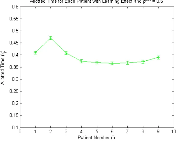
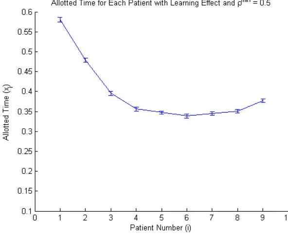
A quick examination of the congestion graphs reveals that for each ρmin value the allotted time for each patient, beginning with patient 2, shows a decreasing trend as they are scheduled later in the day. The decrease in allotted time is most likely because congestion in the office will begin to build up throughout the day as more patients arrive for their appointment. Then, since the model is set up to have patient’s procedure durations decrease by a set factor according to the number of patient’s currently waiting, the assigned allotted time would be less for each patient. Additionally a closer look at the provided graphs (Figures 4.12 - 4.16) shows that there is a correlation between a smaller ρmin value and a larger range of allotted time for patients 2
Figure 4.13: Graph of Patient Allotted Times, in hours, with Congestion Effect, ρmin = 0.8
Figure 4.15: Graph of Patient Allotted Times, in hours, with Congestion Effect, ρmin = 0.6
range of .07 hours is shown between whenρmin = 0.9 and whenρmin= 0.5. Finally a noticeable characteristic of the congestion model allotted time graphs is that the initial scheduled patient is always given the shortest allotted time of all 10 patients, which is reminiscent of the fatigue model.
4.7
Heuristics
In this section we propose some easy to implement heuristics for each of the three server behav-ior models. The heuristics for the learning and fatigue models were determined based on their respective server behavior effect equations. The congestion behavior heuristic was derived from the analysis of the results in Section 4.6.
Below we describe the motivation behind each model heuristic, and support why each ap-proach was selected. Then to understand how effective each heuristic is we compare the mean optimal objective value and 95% confidence interval to that for each of the heuristics. The mean optimal objective values are then compared to those found in Section 4.4 to determine the effectiveness of each heuristic.
4.7.1 Learning and Fatigue Heuristic
The heuristic determined based on the learning and fatigue models is based on the effect equa-tions, 3.1 and 3.2, mentioned in Section 3.2.1. In a situation where a learning behavior is believed to affect appointment times we determined that patient’s appointments could be scheduled based on the following heuristic determining allotted time for each patient:
xi =gLρmin(i)·µi, ∀i. (4.1)
Similarly, for the fatigue behavior model the following heuristic is suggested:
xi=ρminF(i)·µi, ∀i. (4.2)
Table 4.13 shows the mean optimal objective value when a learning effect is present using the 2-SLP learning model, learning heuristic, and ASP model forn= 10 patients and our previously defined service time distribution, U(0,1). Table 4.13 reveals significantly higher values for the heuristic and ASP for all ρmin values when compared to the mean optimal objective value using the learning effect 2-SLP. The difference in means between the 2-SLP and the heuristic are much smaller forρmin≥0.6 with a differences ranging from around 125 to 515, as opposed to ρmin = 0.5 that has a difference of over 1000. It should however be noted that the mean optimal objective values using the ASP are smaller than the mean optimal objective values using the heuristic for ρmin ≥0.8. The lower mean optimal objective values between the ASP and the heuristic suggests that the current heuristic may be ineffective. In some cases however, when the heuristic mean optimal objective values fall below those of the ASP, this may indicate the heuristic may be on the correct path.
Table 4.14 shows the mean optimal objective value when a fatigue effect is present using the 2-SLP fatigue model, fatigue heuristic, and ASP model. Comparing each column reveals
Table 4.13: Comparison of mean optimal objective values for a learning effect using the 2-SLP learning model, learning heuristic, and ASP model.
Learning Effect Mean Optimal Objective Values
2-SLP Heuristic ASP
g0L.9(i) 6521.35 6965.41 6031.39 g0L.8(i) 4288.64 4606.03 4208.216 g0L.7(i) 2469.28 2595.54 2791.14 g0L.6(i) 1165.82 1678.74 1893.42 g0L.5(i) 456.45 1533.83 1304.08
Table 4.14: Comparison of mean optimal objective values for a fatigue effect using the 2-SLP fatigue model, fatigue heuristic, and ASP model.
Fatigue Effect Mean Optimal Objective Values
2-SLP Heuristic ASP
that the fatigue heuristic produces a similar change in optimal objective value as the learning heuristic. The optimal objective value using the fatigue heuristic again returns significantly higher values than the 2-SLP model for fatigue. However, for the fatigue heuristic the difference in means remains smaller for allρmin values with differences ranging from around 130 to 580. Comparing the mean optimal objective values for the heuristic to those of the ASP are not a viable comparison in this case because of a decrease in mean, see Table 4.2. The results for the fatigue heuristic indicate that it may be a more accurate portrayal of the behavior without use of a complicated model, but some adjustments are still needed for accuracy.
4.7.2 Congestion Heuristic
Determining a heuristic for the congestion model was a more difficult task than for the learning and fatigue models, because the congestion model is more complex and therefore has a less intuitive set of results. In order to better understand the results produced by the congestion model a deterministic version of the system was created. The deterministic version of the con-gestion model removes the randomness associated with the stochastic model. Therefore, a more in-depth understanding of the model and the relationship between its variables and solutions may be gained.
The deterministic mean value model was created by replacing the stochastic variables,z(ω), with their mean. Thus, since the probability distribution for each variable was U(0,1) in our experiments, their mean value was 0.5. Using these values the model was run using five different ρmin values,ρmin = 1.0,0.9,0.8,0.7,0.5, in the linear congestion effect function, fρmin(j), and
a varying number of patients,n. The resulting allotted times for each ρmin value and selected n were recorded and examined for patterns. The resulting pattern found that for n ≥ 4 the allotted time for patients 1 throughn−1 could be calculated by the equation:
xi =
1 2−
(1−ρmin) 2(n−1)
i, ∀i. (4.3)
4.8
Conclusions
The experiments for the three server behavior models help to determine several important factors about each model. The learning and fatigue models while similar in formulation have different optimal schedules. It also seems to be that more significant effects are observed with the learning model. Suggesting that learning may have a greater influence on optimal schedule than fatigue. The congestion model has a more significant effect on the optimal appointment schedule compared to the learning and fatigue models, which result from the increased con-straint considerations needed for the congestion model.
The analysis of the sensitivity of the models shows each model’s response when a particular server behavior is present and accounted for, and when the behavior is ignored. The learning and fatigue models have opposing reactions in their resulting optimal objective values in this case. The learning model returns significant increases in the objective function when a learning behavior is present and not accounted for in the scheduling model. The fatigue model suggests a decrease in cost when fatigue is present and not accounted for, however there are no statis-tically significant decreases that can be observed for the specific test cases we considered. The congestion model also returns significant increases in cost when server’s react to the presence of congestion but the model does not consider an effect from congestion. Each of the models also tend to show more significant decreases when the server behavior effect is greater, meaning a smallerρmin value.
Table 4.15: Comparison of mean optimal objective values for a congestion effect using the 2-SMIP congestion model, congestion heuristic, and ASP model. (+ indicates a statistically significant difference between the mean optimal objective values for the heuristic and ASP, where the difference between the mean optimal objective value of the heuristic and the 2-SMIP is smaller than between the ASP and 2-SMIP.)
Congestion Effect Mean Optimal Objective Value
2-SMIP Heuristic ASP
f0.9(j) 7193.90 7738.15 7220.61
f0.8(j) 5635.54 5922.68 5721.61
f0.7(j) 4067.90 4316.86 4320.13
f0.6(j) 2718.07 2896.07+ 3167.03