The Speciating Selection Event Algorithm: Evolutionary Computation Inspired by Darwin's Finches and Sewall Wright.

(1)

Abstract

NICHOLSON, JOHN WELDON. The Speciating Selection Event Algorithm: Evolutionary Computation Inspired by Darwin’s Finches and Sewall Wright. (Under the direction of Mark White.)

Evolutionary computation is a heuristic optimization technique inspired by nature.

The optimization problem is analogous to the natural environment, candidate solutions

become individuals in the population, and relative solution quality determines individual

fitness. Evolution, acting through selection and reproduction, directs the search to find

an optimal solution.

Biologists have studied “Darwin’s finches” on the Galapagos archipelago and found that

the El Ni˜no effect, which causes periodic drought-induced scarcity, and monsoon-providing

abundance, is driving a noticeable genotypic and phenotypic adaptation. I utilize a

periodic selection event, and population growth parameter controls, to simulate this

natural phenomenon. I demonstrate that these mechanisms provide additional efficiency

and robustness to the evolutionary search.

Sewall Wright’s Shifting Balance Theory indirectly tells us that the population size

of a sub-species is proportional to its fitness: more-fit sub-populations will have more

individuals and be in an exploitation mode, while less-fit sub-populations will have fewer

individuals and be in an exploration mode. I use this as inspiration to allocate offspring to

different sub-populations (species) in unequal amounts, through the selection process. The

less-fit species will win fewer offspring, causing them to explore the search space through

weaker selection pressures and random genetic drift. I show that this is a beneficial

mechanism for multi-modal search, granting the ability to escape from local optima, and

(2)

That is, this mechanism helps to achieve an automatic balance between exploration and

exploitation.

These two inspirations are implemented in the Speciating Selection Event algorithm.

I focus on understanding the behavior of the algorithm, and how effectively it is able to

search the problem space. To do this, I make use of conceptually simple mathematical

functions, rather than a real-world or engineering task.

In this work I also analyze the behavior of one of the canonical algorithms in the field

of evolutionary computation, furthering the understanding of the feedback mechanism

through which the problem environment and selection method effect the evolutionary

search. This understanding is also put to use in the analysis of the Speciating Selection

(3)

(4)

The Speciating Selection Event Algorithm: Evolutionary Computation Inspired by Darwin’s Finches and Sewall Wright

by

John Weldon Nicholson

A dissertation submitted to the Graduate Faculty of North Carolina State University

in partial fulfillment of the requirements for the Degree of

Doctor of Philosophy

Electrical Engineering

Raleigh, North Carolina

2011

APPROVED BY:

Mesut Baran Griff Bilbro

Trudy MacKay Mark White

(5)

Dedication

(6)

Biography

I was born in 1980 in Palm Bay, Florida, to my parents, Stuart and Cathy who had moved

to the area from Chicago, Illinois. I am the oldest of three, having a brother, Michael,

and a sister, Sandra. My father is an electrical engineer, so we all grew up with gadgets

and gizmos, not to mention electronics kits. This certainly led my brother and I into the

fields of computers and engineering.

One of my primary extra-curricular activities in high school was the science fair. In

Brevard county the science fair took place at the local mall over a two day period, where

all of the students in the county sat around their demonstration boards waiting for the

handful of judges to come around for a quick presentation and questioning. Though I

was always a procrastinator, and my projects suffered for it, I was always excited and

interested when it was finally time to present. I am sure that this experience led to my

love of academic conferences, and a desire to continue my education in graduate school.

After high school I went on to the University of Florida, obtaining degrees in electrical

and computer engineering in 2002. I did well in my schooling, but for some reason (cough

video games cough) I was not involved in anything extra-curricular, though of course

now I wish that I had been. Over the summer breaks I interned at Aeronix, a small

government contractor in my home town. I was fortunate to work on very interesting

projects, including components for a satellite and a UAV. This reinforced my primary

academic interests as well, focusing on embedded design and digital logic.

My graduate education found me enrolling at North Carolina State University, where

I completed a non-thesis degree in 2004. I entered primarily interested in digital logic

design, but was quickly swayed to neural networks, pattern recognition, and evolutionary

(7)

Ozturk’s Introduction to Electrical Engineering, which was itself a fun and rewarding

experience. I have always agreed with the saying that the best way to understand a

concept was to teach it to someone else (Frank Oppenheimer), and perhaps nowhere is

that more true than in an introductory course.

After completing my Master’s work, I started working full-time at IBM, while

contin-uing the pursuit of my doctorate on a part-time basis. This was my status quo for seven

years, changing employment to Lenovo when IBM sold their PC division, and changing

roles within the company on several occasions.

Most importantly, it was in high school that I met my wife, Erin. She too was involved

in science research (being much better at it than I, by the way), and after spending

time together with various clubs and groups at school, we started dating. We stayed

together through university at different schools, both obtaining our Master’s degrees

(8)

Acknowledgements

I would like to first of all thank my wife, Erin, for all of the support she has provided. I

would not have been able to do this without her.

I would also like to thank Dr. Mark White, my committee chair, for inspiring me to

want to continue my education and get this doctorate, and also for our weekly meetings

over seven years.

I would be remiss in neglecting to acknowledge my committee for their support. My

part-time status was never a problem, and whenever I had a question for anyone a useful

response was never long in coming.

Finally, I would like to thank my management at IBM and Lenovo. They were never

anything but accommodating and encouraging in this entire process, and I will forever be

(9)

List of Tables

Table 5.1 New parameters for the FSE algorithm . . . 84

Table 5.2 Success rates for FSE on ffork . . . 90

Table 5.3 Additional results for FSE on ffork . . . 91

Table 6.1 SSE population control script elements . . . 102

Table 7.1 (µ, λ)-ES results on 5-D flinsin . . . 129

Table 7.2 FSE results on 5-D flinsin . . . 130

Table 7.3 SSE results on 5-D flinsin . . . 131

(13)

List of Figures

Figure 1.1 EC diagram . . . 1

Figure 1.2 Recombination diagram . . . 12

Figure 1.3 Distribution of offspring for σ self-adatation . . . 19

Figure 1.4 Typical lineage illustration for ES algorithms . . . 20

Figure 1.5 Typical loss of diversity for ES algorithms, shown empirically . . . 21

Figure 1.6 Step-by-step illustration of (5,10)-ES . . . 28

Figure 2.1 Sphere and Ridge test problems . . . 32

Figure 2.2 Ellipse test problem, fellipse . . . 34

Figure 2.3 Depiction of what makes fellipse difficult . . . 36

Figure 2.4 Fork-trap test problem, ffork . . . 38

Figure 2.5 Linearly increasing sinusoid test problem, flinsin . . . 40

Figure 2.6 Source of pressure to decrease or increase σ onflinsin . . . 41

Figure 3.1 Empirical end-of-run efficiency of (1, λ)-ES onfellipse . . . 45

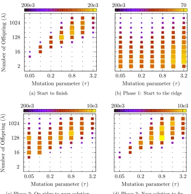
Figure 3.2 Empirical end-of-run efficiency of (1, λ)-ES on fellipse, showing both independent variables . . . 46

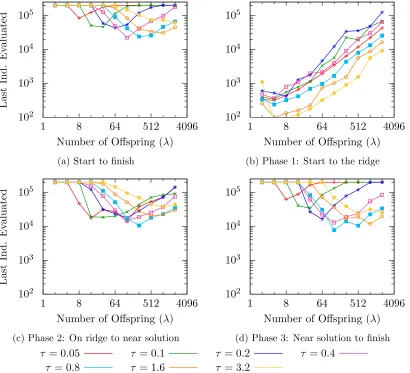
Figure 3.3 Empirical efficiency for combined phases two and three . . . 50

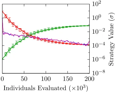
Figure 3.4 Evolution dynamics for (1, λ)-ES on fellipse . . . 51

Figure 3.5 Source of efficiency: e vs ˆσ . . . 54

Figure 3.6 Probability of progress . . . 58

Figure 3.7 Probability of progress, focus on apsis . . . 59

Figure 3.8 Expected values of genes during evolution . . . 61

Figure 3.9 Evolution dynamics with small τ . . . 65

Figure 3.10 End-of-run efficiency with elitism . . . 66

Figure 3.11 End-of-run efficiency with elitism, comparison . . . 67

Figure 3.12 Evolution dynamics with elitism, large τ, and smallλ . . . 68

Figure 3.13 Evolution dynamics with elitism, large τ, and largeλ . . . 69

Figure 3.14 Effect of problem difficulty on end-of-run efficiency . . . 71

Figure 4.1 SE family structure with uniform growth . . . 77

Figure 4.2 SE family structure with non-uniform growth . . . 78

Figure 4.3 Typical evolution dynamics for SE on ffork . . . 81

Figure 5.1 FSE algorithm illustrated step-by-step . . . 86

Figure 5.2 Typical evolution dynamics of the FSE algorithm on ffork . . . 88

Figure 5.3 Typical evolutionary dynamics of each family for FSE on ffork . . 92

(14)

Figure 5.5 How FSE with uniform growth can escape from the trap . . . 94

Figure 5.6 How FSE with uniform growth can escape from the trap, close up view . . . 95

Figure 5.7 Population diversity of SE and FSE . . . 96

Figure 6.1 Demonstration of growth control script in SSE . . . 104

Figure 6.2 Typical evolution dynamics of SSE clustering on ffork . . . 110

Figure 6.3 Demonstration of the benefits of speciation . . . 112

Figure 6.4 Demonstration of a drawback of using a radius-based cluster . . . 113

Figure 6.5 Clustering and caching mechanisms illustrated . . . 115

Figure 6.6 The benefit of caching shown empirically . . . 117

Figure 7.1 Results of the best parameterizations for the four algorithms on 5-D flinsin . . . 121

Figure 7.2 Results of the best parameterization for FSE, long run . . . 122

Figure 7.3 Median and quartile results . . . 125

Figure 7.4 Evolution dynamics of the best lineages . . . 127

Figure 8.1 Fitness sharing depiction . . . 135

Figure 8.2 SBGA depiction . . . 142

Figure 9.1 Algorithm efficiency with increased selection pressure . . . 150

(15)

List of Algorithms

Figure 4.1 The Selection Event (SE) Algorithm . . . 74

Figure 4.2 The Mutate() procedure . . . 77

Figure 5.1 The Family-based Selection Event (FSE) algorithm . . . 83

Figure 6.1 The Speciating Selection Event (SSE) algorithm . . . 99

Figure 6.2 The IntermediateCulling() procedure . . . 100

Figure 6.3 The Growth() procedure . . . 101

Figure 6.4 The Speciate() procedure . . . 106

Figure 6.5 The Cluster() procedure . . . 107

(16)

List of Acronyms

EC Evolutionary Computation

EP Evolutionary Programming

ES Evolution Strategies

FSE Family-based Selection Event

GA Genetic Algorithm

GP Genetic Programming

SBGA Shifting Balance GA

SE Selection Event

(17)

List of Symbols

Parameter Description

a A scalar coefficient, used in some test problems d The problem dimensionality

D Population diversity measure

Fα Growth rate, the number of individuals, a parameter in SE

FA Growth rate when competing with all other individuals in the population, a parameter in FSE

FI Growth rate without competition for selection, a parameter in FSE FF Growth rate when competing with other members of the same family, a

parameter in FSE

g The current generation number Gi The gene at locus i of the genome

Ii Individual i, a member of the population P k Selection pressure (e.g., tournament size), or k An integer, used as a multiplier

LC A limit on the number of clusters, a parameter in SSE N(0,1) One sample from a standard Normal distribution

NF The number of families (also the initial population size), a parameter in FSE

p The size of the population, the number of individuals, in the current generation

p(g) The size of the population, the number of individuals, at generation g P(g) The population, a set of individuals, at generation g

TSE Selection Event period, in generations U(0,1) One sample from a Uniform distribution1 λ Offspring population size in an ES

µ Parent population size in an ES

(18)

CHAPTER

1

Introduction: Evolutionary Computation

Evolutionary Computation (EC) is a heuristic optimization technique inspired by nature.

The problem being optimized is decomposed in such a way that it enables a solution

to be encoded as the genetic material of an “individual”. A “population” of these

individual candidate solutions then go through a selection process, where better solutions

are more likely to be selected, and a variation process that produces new solution-encoding

Select

Reproduce

Evaluate

(19)

individuals. As this process iterates (over the generations), the population is hoped to

evolve into a nearly optimal solution.

These central themes of EC are described in more detail below, but it is worth

mentioning here that the applications of EC are many and varied:

Place and route [15], traveling salesman problem [48] Job scheduling [42]

Antenna design [80] Protein folding [14] Parameter fitting [45]

Robotic neural controllers [92] Artwork [69]

There are many optimization techniques that exist in engineering. The reason to

consider using the evolution analogy is because it offers some advantages over other

methods. One of the principal benefits that it offers is that it is able to simultaneously

solve multiple objectives. For instance, on an antenna design problem, you want to

maximize the response at the intended frequency of operation. At the same time, you

have additional design goals, including directionality, side-lobe minimization, power

efficiency, the physical dimensions, the rigidity and durability, and so on. In a traditional

optimization technique, such as Guass-Newton, Levenberg-Marquadt, or Nelder-Mead, all

of these objectives need to be combined into a single equation. The construction of this

aggregated objective function is difficult to know before-hand, and has a drastic effect

on the result. With EC, it is possible to formulate the multi-objective function directly,

(20)

EC is also more well-suited to use while remaining ignorant of the problem being

solved: so-called black box optimization [36]. If the practitioner would spend the time

necessary to understand the problem they are trying to solve, then better results can be

achieved. In many scenarios, it is preferable to obtain a “good enough” result without

having to spend the time needed to understand the problem in detail. Some optimization

techniques require that this domain knowledge be utilized in order to get a decent result,

but EC is typically quite resilient.

For similar reasons, EC is able to provide possible solutions to problems while

pre-venting practitioner bias from becoming part of the solution. For instance, in order to

understand the problem, it will likely be decomposed into its constituent parts. The

manner of this decomposition can constrain the search in certain ways, precluding the

system from finding a better solution. Alternatively, constraints might be placed upon

the solution that are unnecessary. For example, a physical structure might be biased to

use right angles, when a lighter or stronger structure would be possible otherwise.

Finally, many problems are non-differentiable or otherwise non-smooth. Many

opti-mization techniques do not work in this situation, but EC has no issues with these types

of problems.

1.1 Evaluation

In EC, the paradigm of evolution is used to solve a computational problem through

computer simulation. To do this, the problem being solved is analogously thought of as

the “fitness landscape”, a concept first introduced by Sewall Wright [87]. Individuals in

the environment have a fitness to that environment: salamanders are adapted to living in

(21)

given point in the problem space, as a solution to the problem, is assigned a fitness value.

Points which are better solutions to the problem have a better fitness value. Importantly,

only the relative fitness among individuals is relevant to the evolutionary process, while

the absolute fitness is what matters to the practitioner using this search technique. The

term “problem environment” is also used when referring to the computational problem

being solved.

In problem environments that are mathematical functions, like I use in this dissertation,

the fitness evaluation of an individual is a direct process of determining the value of the

function for the position that the individual represents. This type of environment is used

mostly to study EC algorithms directly. As I mentioned earlier, the motivation for using

EC is in solving the types of problems not always well represented by functions. For

instance, one might use EC to determine how a given protein will fold. This process

requires determining the energy required for the protein to have the given shape; the

minimal energy shape will be the one that the protein folds to in reality. Determining the

energy state of a given shape is a very computationally intensive and time consuming

task, but this is necessary to determine the fitness of any given shape. In recognition of

this, algorithm efficiency is determined using the number of individual evaluations, or

function evaluations, required to solve the problem.

Another approach that is used to evaluate the fitness of a candidate solution is to

somehow determine the relative fitness of the individuals in the current population. This

the only reason the evolutionary system needs the fitness values in the first place; evolution

doesn’t care how well a new wing design performs aerodynamically, it only needs to know

the relative performance of the candidate wing designs, in order to know which ones to

favor in selection. Because of this, practitioners often use a heuristic approach to assign

(22)

Alternatively, the fitness can be estimated by a type of tournament, in which the

individuals in the population compete against each other as solutions to the problem.

This approach is often necessary when it is not obvious how to evaluate the quality of

a solution. One such example is the evolution of a checkers player [27]. How does one

know what is a good way to play checkers? If the candidate solutions all play checkers

against each other, then an estimate of their quality can be obtained. This approach is

also sometimes thought of as the establishment of an evolutionary arms race – something

that occurs in nature as well [19].

1.2 Encoding

The individuals in the evolutionary simulation represent a particular candidate solution to

the problem being optimized. In order for evolution to work, the position of the individual

in problem space needs to be encoded in such a way that it is heritable by the offspring

of the individual.

In the EC analogy, the phenotype of the individual is everything which is directly

used to evaluate the fitness of an individual: their position in the problem space. The

genome of an individual, which is used during reproduction, can contain more or different

information. In the simplest case, the genotype is identical to the phenotype, in which case

the only information in the genome is a direct encoding of the position. Or, the genome

can contain additional information than that which is required only to represent the

position; for example, the genome may contain values which govern mutation. Additionally,

more complicated relationships can be involved, such as information on how to build

the phenotype (e.g., a neural network), or how to build a juvenile individual, if the

(23)

(artificial embryology) [53].

One of the key factors in the quality and speed of the evolutionary search is how the

problem is encoded into genetic material. For example, a common approach in EC is to

use bit strings as the genome; groups of adjacent bits are often combined to represent a

real-valued number using fixed-point notation. In this configuration, the genes have very

different effects on the position: the most-significant bit has twice the effect of the next

bit, and so on in exponential fashion. When a bit-flip mutation occurs in this encoding,

the effect can be dramatic. However, by utilizing a reflected binary code, or Gray code, a

single bit change cannot be so disruptive. This is just an illustration of the concept; some

problem environments can see much improved performance through careful or creative

encoding techniques.

Beyond encoding, the location of each gene can be important. In problems with

interacting dimensions, analogous to epistasis in the biological context, if these genes

are located adjacent to each other, or even near to each other, the EC algorithm will

typically perform better than if they are far apart. This is because when the genes are

close together, they are less likely to be disrupted by recombination [31]. This concept is

also related to the idea of genetic linkage; if genes are strongly interacting, we would like

to artificially link them, so that they are not disrupted [39].

This dissertation uses a direct encoding of real-valued numbers, specifically

double-precision floating points. Each dimension of the mathematical function being optimized

(24)

1.3 Selection

In order for the computational search to drive the evolutionary system towards more

promising solutions, the selection process is implemented. The individuals in the

popula-tion have each had their fitness determined by taking the solupopula-tion that is encoded in their

genome and evaluating it for the problem at hand. Now, those individuals with better

fitness need to somehow be picked such that when new individuals are produced they are

given the best chance of finding further improvements in the solution. In EC there are

three common selection methods. While there are many others, those described below

are the three most frequently used.

Fitness proportionate selection, sometimes called roulette wheel selection, assigns a

probability of getting selected to each individual, where the probability is proportional

to the fitness of the individual: the most-fit individual in the population at the current

generation has the most likelihood of being selected. Fitness proportionate selection

sometimes requires tuning for each problem environment. It is often necessary to use

the logarithm or antilogarithm of the fitness value to scale the probabilities for good

algorithm performance, otherwise the probability might be spread too evenly across all

individuals of the population, which is akin to random selection, or the probability might

be too concentrated at the most-fit individuals, leading to premature convergence due to

allele fixing.

An often used alternative to fitness proportionate selection is tournament selection1_,

in which some number of individuals are randomly selected from the population, and

then engage in a “tournament”. The most-fit individual competing in this tournament is

the one that is selected. The stochastic nature of this method comes from the random 1_{Tournament selection is not to be confused with the use of a tournament to assign fitness to individuals,}

(25)

selection of individuals; the size of the tournament, or number of samples, reduces this

effect and makes it more likely that the selected individuals will be the ones with higher

fitness values.

Truncation selection is the third common type of method used. This method is entirely

deterministic: the population is simply truncated to the n most-fit individuals.

Selection is also a competition: a competition for offspring, or for survival, depending

on how the method is used. In the artificial evolution domain, things that are impossible

to do in nature can be simulated, such as provide three offspring to every individual, and

use the selection routine to determine which of them survive.

1.3.1 Competition-free Selection

Consider the situation where there is never any selection in the population. No individuals

ever have to compete: they just make one or more offspring every generation, and no

individuals ever “die”. This leads to unbounded growth, and pretty quickly at that.

From a computational perspective this algorithm is horribly inefficient and impossible to

implement due to finite computer resources.

Since it is impossible to be competition-free, there has to be some competition in the

system. That is, there must be some form of selection.

1.3.2 Selection with Global Competition

The most straightforward and typical method is to compete a population of parents with

each other to produce a population of children, which can be larger, the same size, or

smaller. In order to make the parent population of the next generation, there may be

(26)

of almost all evolutionary algorithms, but it has some notable problems.

The process of choosing those individuals who survive and make it into the next

generation can produce a very large selection pressure on the population. Goldberg’s

“takeover time analysis” [31] shows that, in the absence of all variational (e.g., recombination

and mutation) operators, the selection operator will remove all diversity in the population

in the order of ln(p) generations, with p the population size. This is the result when all

diversity is lost; large amounts of diversity can be lost in a single generation or two. This

loss of diversity leads to premature convergence – where the algorithm has converged to

a problem solution that is suboptimal, and has no way of improving because all of the

alleles are fixed.

1.3.3 Selection with Restricted Competition

So if global competition has these drawbacks, what is the alternative? The competition

must be limited in some way.

By far the most common method of limiting the competition is through the use of

a metric on the phenotype of individuals. One such method is “fitness sharing” [30].

This mechanism works by diminishing the fitness value of an individual proportionally to

the number of other individuals who are nearby, given some metric. The motivation for

this approach is that because of the fitness sharing, evolution will produce individuals

which are more spread out from each other than they otherwise would be, thus promoting

population diversity.

Another common approach is to isolate sub-populations, and allow them to intermingle

in some manner, but infrequently. One example of this is parallel genetic algorithms [33],

(27)

having several isolated populations, with an occasional migratory individual. Because the

sub-populations evolve in relative isolation from each other, they are free to evolve into

different areas of the search space. The migrant is typically the best individual from each

island, and is sent to each of the other islands. There are many ways to alter this setup

including different connectivities between islands and asynchronous migrations.

A more rare approach, which I take, is to use the ancestry or lineage of the individuals

to restrict the competition. My algorithms (Selection Event (SE), Family-based Selection

Event (FSE), and Speciating Selection Event (SSE)) will be discussed later, in Chapters 4,

5, and 6.

1.3.4 Other Alternatives

Other ways to maintain population diversity besides restricting the competition are a high

mutation rate, restarting, and random immigrants. Typically in EC the initial population

is entirely random. Having a sufficiently high mutation rate to overcome the diversity lost

through the selection operator and genetic drift is the traditional method of preventing

premature convergence, but it is quite ad hoc and requires tuning for every new problem.

Another common approach to the problem of premature convergence is to simply

restart the search, keeping the best-found individual from the previous search as one of

the new initial individuals. This is similarly ad hoc, though it does not require parameter

tuning and tends to work better in practice. Recent work attempts to use the search

history to guide the restart, improving black box optimization without tuning [17].

An amalgamation of these two ideas is to have what is called a random immigrant.

This is where with some period a new completely random individual is added to the

(28)

1.4 Variation

The variation process is a fundamental operation of artificial evolution, and the primary

aspect that makes EC different from other heuristic search techniques. This process is

responsible for creating new candidate solutions, based on the current ones; when this

process is working, the new individuals constitute an improved solution to the problem.

The typical operations of the variation process are mutation and recombination.

1.4.1 Recombination

The recombination operator in EC takes two or more individuals as parents, and recombines

their genetic material to produce an offspring. When we think of biological reproduction,

this is typically the manner of operation that comes to mind. Since this process requires

more than one parent individual, this is sometimes also called sexual reproduction2_.

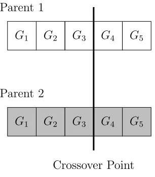
Recombination is used in EC in many forms. In its most basic form, recombination is

implemented as single-point crossover, where the genomes of two parents are lined up,

and a random crossover point is chosen. The offspring then gets the left-half of its genome

from one parent, and the right-half from the other parent.

This concept has been extended to multi-point crossover3_{, uniform crossover}4_{, and other}

mechanisms. Alternatively, other operators such as intermediate or simplex recombination

can be used.

The genetic encoding (see Chapter 1.2) will often determine what recombination

method is used. The gene locus based crossover methods briefly mentioned above may not

2_{Note that sexual reproduction should not be confused with ploidy; almost universally the individuals}

in EC are haploid.

3_{Multi-point crossover is a simple extension of single-point crossover, where}_n_{random gene loci are}

chosen.

4_{Uniform crossover utilizes a probability to determine from which parent the gene value should be}

(29)

Parent 1

G1 G2 G3 G4 G5

Parent 2

G1 G2 G3 G4 G5

Crossover Point

Offspring

G1 G2 G3 G4 G5

Figure 1.2: A diagram of the recombination operator.

apply in a particular encoding scheme, such as ordered encodings used for the travelling

salesman or knapsack problems.

In this dissertation, recombination is not studied. I believe that recombination is a very

beneficial component of EC, and my work could be extended to include recombination

with great utility.

1.4.2 Mutation

The other variation operator is mutation, in which a random perturbation of the genetic

material is performed. The encoding of the problem (see Chapter 1.2) determines the

nature of the type of perturbations that are possible. For instance, in binary string

encodings, the perturbation can be a bit flip, while ordered encodings often swap the

position of two elements.

Since this process is performed on a single individual, it is also called asexual

reproduc-tion when used in the absence of recombinareproduc-tion. However, it should also be remembered

(30)

means.

EC algorithms typically also make use of a mutation rate parameter, which governs

the chance that a particular gene locus will be mutated in the process. In asexual

systems, which rely only on mutation for their source of variation, the mutation rate is

almost universally one, and the amount of mutation is determined by another parameter

controlling the strength of the mutation. Sometimes the strength of the mutation is also

called the step size.

Mutative Self Adaptation

Typically the strength and direction of the mutation are updated by the evolutionary

process. When the parameters controlling mutation are present in the genome of each

individual, it is called self-adaptation [73]. This means that the parameters which control

the mutation of the position in the search space themselves need to be mutated. This

second level of mutation typically uses a separate mechanism, and a fixed parameter.

The origin of this mutative self adaptation was in the context of a real-valued gene

encoding, which will be employed for the remainder of this section. With self-adaptation,

the genome of an individual consists of some values which encode the position in the

search space (x), as well as these new parameters which govern the mutation process.

There was originally some discussion over whether the mutation governing values should

be mutated “first” (or before mutating the position values) or “last” [29]. Since the

position values alone directly determine the fitness of an individual, the consensus is

that the “first” method is the correct one. Using the newly updated governing values

provides some small assurance that these values themselves are not very bad ones for the

production of new offspring.

(31)

latched on to the use of Gaussian mutations. Schwefel [74] and B¨ack [8] suggest

self-adapting the standard deviation parameters that are used to sample Gaussian random

variables used as the mutation steps. These values serve as mutation strength parameters:

larger values lead to greater change in the problem-domain values5_{. There has been}

some work incorporating other distributions, such as Cauchy [54] or L`evy [56], but the

consensus is that the best distribution to use is problem dependent.

When talking about Gaussian distributed random variables in more than one dimension,

one is talking about a covariance matrix (Σ). This can have many parameters, growing as

the square of the dimensionality. Since each one of these parameters must be self-adapted,

in each individual, this is problematic. A trade-off can be made to reduce the number of

parameters, at the expense of generality. B¨ack [8] breaks this down into four categories:

Having only a single σ, i.e., Σ =σI. This is also called isotropic mutation. This method does not allow for variances or covariances to be learned, but does allow a global “step size”.

Having a single dominant axis with its ownσ value and which is allowed to point in an arbitrary direction (requiring d₋1 rotation angles), while the remainder of the dimensions get a common σ and cannot be rotated. This method is mentioned in B¨ack’s taxonomy, but is not used commonly in practice.

Having d σ values but no rotation. That is, Σ is a diagonal matrix, Σ = diag(σ). Using this approach, learning variance is possible, but not covariance.

The full covariance matrix (which is symmetric).

In [51], Kita does an empirical comparison of these four categories of self-adapted

mutation strength algorithms, though without a thorough examination of parameters

(i.e., for a single value of µ, λ, τ, the initial value of σ, etc.). Among other things, he

finds that the full covariance matrix method does well until the problem dimensionality

(32)

increases past 10, at which point the abundance of parameters in each individual becomes

too many for evolution be able to tune.

Theoretical work on the behavior of Evolution Strategies (ES) is most often done

while using isotropic mutations. Meyer-Nieberg and Beyer, in [63], find that in many

problems σ is forced to be small due to competing objectives. That is, σ wants to be

large in order to increase fitness by making big steps in the problem dimensions where

this is appropriate. At the same time, σ is forced to be small in order prevent loss of

fitness by moving away from a known peak.

Hansen [35] discusses the evolutionary dynamics of the self-adapted σ – something

that I have long found to be useful to investigate, and which I discuss in detail in this

dissertation.

Mutative Self Adaptation Controlling Parameter

I mentioned above that the control of the update of σ values is done using a fixed

parameter value. This parameter still needs to be set, and it still has a significant impact

on the performance of the evolutionary algorithm.

In all of my research, I have found that other literature using mutative self-adaptation

often uses the rule for choosing the τ parameter value that is derived in [12]. Beyer

uses the (1, λ)-ES and the sphere model to investigate the details of the behavior of self

adaptation. In his article, Beyer derives the rule for the learning parameter τ initially

outlined in [9]. Namely, that τ is inversely proportional to the square of the problem

dimensionality, and having a “progress coefficient” as a function of λ:

τ = c√1,λ d ∝

√

(33)

Though this relationship is derived only for isotropic mutations on the sphere

minimiza-tion problem, other practiminimiza-tioners are using the equaminimiza-tion directly, typically even ignoring

the progress coefficient. For instance, Kita [51] uses τ = (√2d)−1 _{for several different}

problems6_{, in several dimensions. Other examples of literature using this relationship}

directly include [26] and [58].

Perhaps the reason that others use Equation 1.1 directly is that Beyer argues the

sphere model applies locally in non-sphere problems. I believe that while this may be

true, an insufficiently large value of τ leads to premature decrease in the value of σ, and

very slow, inefficient progress towards the solution. It also remains to be studied how

τ sizing should be done when used with multi-modal problems. In Chapter 3, I report

on the results of an empirical study of the effects of τ on algorithm performance for a

different problem: the highly eccentric ellipse.

Alternatives to Mutative Self Adaptation

Though the full covariance matrix is never self-adapted in practice, the covariance matrix

adaptation ES (CMA-ES) was proposed by Hansen and Ostermeier in [38] as an alternative

to the trade-off outlined in B¨ack’s taxonomy. In CMA-ES, the covariance matrix is built

using data obtained collectively from the population, instead of being self-adapted in each

individual. This algorithm is one of the best performing algorithms in EC, over a wide

range of problems, and has been successfully utilized in hundreds of applications.

Other alternatives to self-adapted mutation strength schemes exist as well. In [5],

Arnold et al. describe a hierarchically organized ES for step length adaptation. In this

approach, the value of τ is updated, but on a slower scale than the other parameters (for

example, every 20 generations). Arnold compares this method against several others in

(34)

[6].

Method Used in this Dissertation

In this work I use the common mutative self-adaptation method which consists of d

independent σ values corresponding to the diagonal of the covariance matrix, the third

in B¨ack’s taxonomy. The genome for each individual contains the individual’s location

in the problem-domain space and these self-adapted strategy parameters. Specifically,

the genome is the concatenation ofx, the position values used in calculating the fitness

of the individual, andσ, the corresponding “strategy-domain” values used in producing

new offspring. The update mechanism is given by

σ+_i = σiexp (τ N(0,1)) (1.2)

x+_i = xi+σ_i+N(0,1) (1.3)

where N(0,1) represents one sample from a standard Normal random variable, iis the

gene index (the genome contains onexand oneσ gene for every dimension of the problem

(d)), the+ _{superscript indicates the gene value of the offspring, and} _τ _{is a fixed parameter}

used in the update of σ.

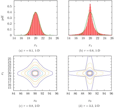
Offspring Distribution

Although the position of each offspring is just a Gaussian perturbation of the position of

the parent, taken collectively all of the offspring are not distributed Normally because

each offspring’s position is determined after updating σ first. The deviation from Normal

is particularly significant for large values of τ, where the σ values can change greatly

(35)

offspring, overlaid with a Normal distribution which would have determined the offspring

positions if τ were 0.

As one can see, whenτ is small (Figure 1.3a) the offspring distribution does not deviate

from the Normal very much, but for large τ (Figure 1.3b) there is a marked difference:

not only are the tails fatter, but offspring are also more likely to be very much like the

parent, not changing the position value much at all. This also has a profound effect

on the multi-dimensional distribution (Figure 1.3c). With a Gaussian distribution, the

contours of probability density are elliptical (circular if the individualσ values are equal)

– but with fatter tails this changes to something star shaped. Even when constrained to

isotropic mutations, this effect is seen for large values of τ. The two dimensional figures

would still be circular, but compared to Normal the contours would be denser near zero

and more spread out further away, corresponding to the same observations made in the

one dimensional plot 1.3b.

1.5 Population

The population consists of all of the individuals in the current generation – all of the

potential solutions to the problem being solved. In EC a population of solutions is

maintained not only in order to have an assortment of solutions to recombine, hopefully

to produce novel solutions, but also to provide a gradient against which selection can

operate. When all of the diversity is gone from the population, you are effectively left

with a single solution.

One of the principal problems of canonical EC algorithms is the rapid fixing of alleles

and loss of population diversity caused by the selection operator. This is analyzed by

(36)

0 0.1 0.2 0.3 0.4 0.5

14 16 18 20 22 24 26

p

df

x1

(a)τ= 0.1, 1-D

14 16 18 20 22 24 26

x1

(b)τ = 0.8, 1-D

15 16 17 18 19 20 21 22 23 24 25

84 86 88 90 92 94 96

x1

x0

(c)τ = 0.8, 2-D

84 86 88 90 92 94 96

x0

(d)τ = 3.2, 2-D

Figure 1.3: The distribution of offspring’s position in the common update scheme. (a) For small values ofτ (which governs the update ofσ), the deviation

(37)

Figure 1.4: A typical lineage of the initial individuals in canonical ES algorithms. Starting from five initial (generation 0) individuals at the top, each level down represents the parent population in a subsequent generation. This particular result is for the (5,10)-ES on theffork problem, but this type of behavior is common.

lineage of the population: a family tree. Figure 1.4 depicts the family tree from a typical

run of an ES algorithm. The top row shows the five initial individuals in the parent

population at generation 0, the second row shows the parent population at generation 1,

and so on. This figure shows that the initial diversity of the population is quickly lost.

This is due to the global nature of the truncation selection used canonical ES algorithms.

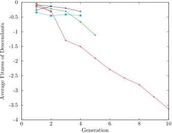
Figure 1.5 depicts this effect in another way, showing typical results of a (10,20)-ES

simulation. Each line gives the average fitness of the individuals in the offspring population,

grouped together by their ancestry. That is, if individuals are descendants of the same

initial individual, they are grouped together for averaging.

The FSE algorithm counteracts this loss of diversity by preventing the death of these

lineages. That is, the last remaining descendant of an initial seed individual is guaranteed

to have at least one offspring. This is explained in more detail in Chapter 5.

In order to study and compare EC algorithms and their effect on population diversity,

(38)

-4 -3.5 -3 -2.5 -2 -1.5 -1 -0.5 0

0 2 4 6 8 10

Av

erage

Fitness

of

Descendan

ts

Generation

(39)

is called the all-possible-pairs population diversity measure [85]. This value gives the

average distance from one individual to all other individuals in the population, averaged

across all individuals in the population. Equation 1.4 gives the definition.

D= 2

p(p₋1) p−2 X

i=0 p−1 X

j=i+1

dist(Ii, Ij) (1.4)

1.5.1 Population Sizing and Varying

Algorithm efficiency and solution quality are significantly impacted by the population

size. This parameter is typically fixed and set a priori, though many have noted that in

nature the population size is one of the most fluid measures of biology, varying more than

other parameters, such as mutation strength. There exists in the literature a plethora of

research that investigates the population size; but almost all of it does so in isolation of

all other parameters.

Some research tries to determine the optimal population size by trying out several

values dynamically, while the simulation is running, and using the one with the best

results. In [43], Herdy implements a two level hierarchically organized evolution strategy

where the lower level operates only on the problem-domain values, and follows the core

evolutionary paradigm of selection and variation in every generation. The level optimizing

the population size is subjected to selection and variation less frequently, only after a

number of function evaluations, chosen to be large enough to allow the lower level to

evolve for several generations. With this method, Herdy is able to adapt the population

size and note the “optimal” value uncovered during the simulation.

The parameter-less GA [40][18] was an attempt by Harik and Lobo to remove many

(40)

creates a race between multiple populations, each one having twice as many individuals as

the previous population. Populations are stopped when a larger population shows better

average fitness (given equal number of fitness evaluations), or the population stagnates

and is unable to make further progress.

In [16], Costa et al. empirically compare fixed-size population GA for several values of

population size, with a varying population size GA (RVPS) of their own design. They find

that using an algorithm which determines an appropriate population size dynamically is

beneficial over an arbitrary choice of population size, but that an optimal static population

size can be found which will out-perform the dynamically learned value.

Another approach involves trying to remove the necessity of a population size parameter

by changing the paradigm. Arabas et al. [3] offer an algorithm (GAVaPS) which has no

specific population size parameter, and instead introduces the concept of an individual’s

lifetime, which is determined at birth based on the fitness value. As such, the population

size is not constant and may vary.

Yet another tact is to identify some other measure which indicates healthy evolutionary

search, associate this measure with the population size, and then implement a mechanism

to change the population size such that the measure is maximized. Hansen et al. [37]

devise a scheme to self-adapt the population size such that the serial rate of progress, or

the expected improvement in fitness per individual, is maximized. The authors found that

the rate of progress was maximized when the second-best individual’s fitness improvement

had an expected value of zero. Using this knowledge, they devised a scheme to adapt the

population size so that this value was maintained.

Huang and Chen [46] attempt to maintain diversity in the population by increasing

the parent population while holding the size of the offspring population constant. This

(41)

operator: as µ is increased the selection pressure is reduced, which the authors argue

allows for population diversity.

Yu et al. [91] use a linkage-learning method to detect building blocks in the problem

encoding, then adjusts the population size to maintain building block supply (initially) and

mixing (later). In [55], Laredo et al. use the building block supply work of Goldberg [31]

to set an initial population size that is large enough. Thereafter the population size is

shrunken in a deterministic fashion, irrespective of the algorithm performance.

Affenzeller et al. [1] discard offspring that are in some sense not fit enough, preventing

them from possibly becoming parents in the next generation. That is, their µ varies

while the number of offspring produced is a constant proportion of the number of parents,

λ=kµ.

Finally, simply analyzing the population size and determining how it affects

perfor-mance under various conditions, is commonly done. Arnold and Beyer show that having a

parent population greater than one is useful in the presence of noise [4], but not otherwise.

Parent and offspring population sizes, in the context of dynamic or time-varying

problems, are discussed by Schoenemann [71]. He pays particular attention to how well

the algorithm does at tracking the optimum once it is found, even allowing the algorithm

to start at the optimum.

In [47], Jansen et al. focus on offspring population size and its effect on the efficiency

of the evolutionary search. Their work is in the domain of binary strings, and concentrate

their efforts on theoretical analysis of the algorithm, rather than an empirical one.

Mallipeddi and Suganthan [60] show the empirical results of their algorithm with fixed

population size, but they also conduct several experiments with different population sizes

in order to determine an appropriate value.

(42)

size, I find them collectively to be lacking in some of the fundamental analysis of the

detailed algorithm behavior that can lead to general and effective algorithm changes. Also,

many times the effect of the population sizing parameters are taken in isolation from

other parameters. In Chapter 3, I focus on analyzing thebehavior of the algorithm, and in

investigating the interaction between two particular parameters, the offspring population

size in a (1, λ)-ES and the self-adapted mutation strength parameter τ.

1.6 The Canonical Algorithms

The field of EC started in several different sub-fields, and was only brought together

under one umbrella later; even though EP and ES are quite similar, they were developed

independently for over 30 years, only coming into contact before a conference in 1992.

Fogel is attributed with the first use of simulated evolution in his Evolutionary

Programming (EP) [28], in 1960. EP algorithms typically have each of p individuals

produce an offspring – i.e., selection free – and then determine the parents of the next

generation by considering both the offspring and parents which generated them. Fogel’s

original work used the evolutionary process to produce better finite state machines than

could be devised manually.

Rechenberg and Schwefel championed Evolution Strategies (ES) [68][72], in the early

1960s. Their early work was in the field of aerospace dynamics. The algorithm that they

devised was to create a new individual as a random perturbation of the current individual,

and replace the current value if the new one is better. This original procedure has been

extended such that today the population size is broken into two parameters: the number

of individuals that are allowed to reproduce (parent population, µ), and the number of

(43)

Holland devised the Genetic Algorithm (GA) [44] in the early 1970s. Whereas EP

and ES used real-valued numbers as their fundamental gene type and are characterized

by their use of mutation as the sole variation operator, GA uses the bit string for the

genome, and recombination as the primary source of variation. Holland also treated the

population size as a constant: p individuals recombine to producep offspring, which are

typically all present in the next generation. Holland was working on cellular automata,

which are a mathematical construct that can produce complex behavior from simple rules.

Finally, in 1992 Koza popularized Genetic Programming (GP) [52]. In this technique,

a “program” is evolved as a tree structure, using elementary components such as addition

and subtraction. This work has also been extended to evolve source code directly, using

computer assembly language.

There are additional related fields that use biological inspiration to solve engineering

problems, such as ant colony optimization [23], particle swarm optimization [49], and

artificial immune systems [25].

Evolution Strategies (ES)

The work presented in this dissertation is derived primarily from ES, so it is worth going

through this procedure in more detail. The canonical (µ, λ)-ES consists of the following

steps, also illustrated in Figure 1.6:

A parameterized number of starting individuals (µ),

who compete (using tournament selection) amongst each other (with replacement) to produce a parameterized number of offspring (λ),

only theµ most fit (truncation selection) of which survive to become the parents of the next generation.

(44)

The use of tournament selection in step 1.6 is what is used in this work; most typically

(45)

1. Start withµ= 5 individuals at the start of each generation.

2. The production of offspring by tour-nament selection starts by randomly choosing two individuals from the pop-ulation.

3. The selected individual with the higher fitness is assigned an offspring.

4. The next offspring is produced in the same manner; tournament selec-tion with replacement is used to deter-mine the parent.

5. Again, the selected individual with the higher fitness is assigned an off-spring.

6. This process is repeated until all λ

offspring are produced.

7. After all offspring are produced, the

µmost-fit of these offspring are found through truncation selection. These are the parents in the next generation, and the whole process repeats.

(46)

CHAPTER

2

Test Problems

In this chapter, the problems used in this dissertation are described. I am using

mathe-matical functions because I am primarily interested in understanding and analyzing the

behavior of the evolutionary algorithm itself, and mathematical functions are the most

convenient to use. The specific problems described on the following pages are used because

they are easy to understand themselves, so the task of understanding and communicating

what the evolutionary algorithm is doing becomes considerably easier.

I first describe the fellipse problem (see Chapter 2.1), which is a unimodal function

used as a minimization task. By specifically using it in a highly eccentric configuration,

one axis of the problem is far more significant than another; by rotating the problem such

that the two problem dimensions are interacting, the problem enables an understanding

(47)

sphere and ridge functions, which are very commonly used to do similar work on the

fundamental understanding of the algorithms.

Most real-world problems of interest are multi-modal in nature, which is in fact one of

the primary motivations for utilizing Evolutionary Computation (EC) in the first place.

To investigate the performance of the algorithms I have devised, I use a simple trap

function, ffork, which is a piecewise linear function that has two peaks, one of which is

more fit than the other. The less-fit peak is more attractive to the evolutionary systems,

making this a deceptive trap problem. I use this simple problem, which is described more

thoroughly in Chapter 2.2, in order to thoroughly examine the behavior of the algorithm.

Finally, I test the understanding of multi-modal search on another problem. flinsin is

a linearly increasing sinusoidal function having multiple peaks, each one in succession

more fit than the previous. This test problem is used in multiple dimensions to more

exhaustively examine algorithm performance, compare results, and show the benefits of

the algorithm changes. Refer to Chapter 2.3 for more details.

2.1 Ellipse

As was mentioned in the introduction to this chapter, a highly eccentric rotated ellipse

problem is used to investigate the behavior of the evolutionary algorithm. I use this

function to examine the behavior of the canonical Evolution Strategies (ES) algorithm in

Chapter 3. This type of analysis is typically done using the sphere or ridge functions, but

the ellipse effectively combines both of these problems into one, allowing the investigation

of some additional behaviors. Others have started to use the ellipse for this purpose as

well [61].

(48)

sphere problem is so-called because the contours of the function are hyper-spheres; the

min-imization task is given in Equation 2.1 and depicted in two dimensions in Figure 2.1a. The

sphere task is easy to understand, which makes analyzing the EC algorithm performance

somewhat easier, but greatly enhances the ability for the findings to be communicated

to others. Beyer [12] does much work in this area, using the increasing curvature of the

problem as individuals get closer to the origin to determine the optimal value ofσ, among

many other things.

fsphere(x) = d−1 X

i=0

(xi)2 (2.1)

fridge(x) = x0 −a d−1 X

i=1

(xi)2 (2.2)

The ridge function (Equation 2.2, Figure 2.1b) is similarly easy to understand, also

furthering the understanding of algorithm behavior. This problem is an unbounded

maximization task. The sphere minimization task is coupled with a simple linear function;

the best fitness is achieved when increasing this linear dimension of the problem while

holding all of the other dimensions to zero. In order to prevent this problem from becoming

trivial, isotropic mutations are used. This means that there are competing “forces” on

the strategy parameter σ: a large σ allows the system to produce offspring that quickly

increase the linear dimension, but all of the other dimensions requires a small σ value

so that they remain close to zero. The most efficient value of σ is determined by the

interaction of some parameters which control how sharply the fitness decreases when

moving away from the ridge.

(49)

-3 -2 -1 0 1 2 3

x1

x0

(a)fsphere contour plot

-3 -2 -1 0 1 2 3

0 2 4 6 8 10

x1

x0

(b)fridge contour plot

(50)

the optimum, the greatest feedback from the environment is to get close to the major

axis of these concentric ellipses, like the ridge function. After the ridge is found, fitness

improvement is available by proceeding along this axis while not deviating far from it,

also like the ridge function. Eventually the system will approach the minimum and have

to take ever smaller steps, like the sphere minimization task.

A contour plot of this fitness function is composed of concentric ellipses. The fitness

function (Eq. 2.3) is illustrated in Figure 2.2. The basic fitness function can be shifted

(by o) and rotated (byR).

fellipse(x) = s

X

i

(aizi)2 (2.3)

z = R(x₋o) (2.4)

When the ratio between the two coefficients is large (see Figure 2.2c and 2.2d), and

because the evolutionary system treats the problem domain values independently, the

solution to the problem occurs sequentially in three “phases”. The first phase is the

computationally easy one: finding the “ridge” (i.e., the semi-major axis of the concentric

ellipses). Even though there is some feedback from the fitness function about improvement

in the less weighted dimension, it is less important. Because there are only a limited

number of individuals to sample the fitness function, the evolutionary process will almost

always select the offspring which is closest to the ridge, without regard to the offspring’s

location on the minor axis. Only rarely would the offspring’s location along the minor

axis have an impact on selection. Once only small improvements can be made on the

heavily weighted axis, evolution has found the ridge and the first phase is over. The

(51)

-100 -50 0 50 100

x1

x0

(a) Not shifted, Not rotated, low ec-centricity (a= [1,2])

-100 -50 0 50 100

x1

x0

(b) Shifted, Rotated, low eccentricity (a= [1,2])

-100 -50 0 50 100

x1

x0

(c) Shifted, Not rotated, high eccen-tricity (a= [1,100])

-100 -50 0 50 100

x1

x0

(d) Shifted, Rotated, high eccentric-ity (a= [1,100])

10 20 40 80 160

(52)

the more computationally difficult task (again, given the independent treatment of the

problem-domain values). Not so obvious is a third phase to the problem which only

becomes evident when examining the simulation results closely. This third phase involves

the (surprisingly large) computational effort required to go from near the optimum to a

couple of more orders of magnitude closer. More on this topic later.

In short, the evolutionary system will optimize the “true” (rotated) dimensions

sequentially, with the first phase involved in optimizing the more important dimension,

and the second phase spent optimizing the less important dimension. What makes the

second phase difficult in this case is the fact that the update mechanism is forced to

treat the axes independently, when the problem has a strongly dependent relationship

between the axes. If this dependence relationship were allowed to be learned (e.g., having

a self-adapted parameter that represents, and adjusts for, this interdependence), then

progress in the search process could occur along both “axes” simultaneously. More than

that, though, the gains made in the more important axis could be learned (and “locked

in”) by decreasing the corresponding σ value and preventing this progress from being lost.

All of the experiments in this dissertation use a two dimensional version of the test

problem, with the axes rotated 45◦_{, with the minimum translated to (40}_,_{70), and with}

a large coefficient ratio (1 : 100). Figure 2.2d illustrates the function used for the

experimental simulations.

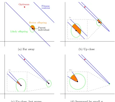
In order for the simulation to progress towards the solution, the parent must produce

at least one offspring which is more fit than itself. That is, the offspring is placed inside

of the line of iso-fitness for the parent; and, for this problem, the iso-fitness contour is an

ellipse. Figure 2.3 depicts the situation.

As can be seen from Figure 2.3a, the contours are essentially straight lines (at 135◦_),

(53)

Optimum

Fitness contour

Parent individual

Likely offspring

Better offspring

(a) Far away

2x

(b) Up close

2x

(c) Up close, but worse

16x

(d) Improved by smallσ

(54)

at the beginning of the problem (at (0,0)) and throughout phase one of the problem, the

probability of producing an offspring with a better fitness value is _≈0.5. Then, during

phase two, two things occur which make the problem more difficult. First, for large values

of σ, it becomes possible to produce offspring that are worse than the parent by moving

“too far” (see Figure 2.3b). Second, and far more damaging to progress, it becomes

necessary to create offspring in a specific direction (see Figure 2.3c). This directional

requirement eventually becomes a necessity in order to solve the problem, because as one

gets closer to the solution, one moves further towards the apsis of the ellipse.

2.2 Real-Valued Trap (1-D)

In order to investigate the fundamental behavior of the algorithms in a multi-modal

problem space, a piece-wise real-valued trap problem is defined in Equation 2.5, subject to

the constraints in Equation 2.6. These constraints ensure that from the starting position

(atxb) the left fork (followingmb) is more attractive than the right fork (followingmc).

Since canonical EC algorithms work locally, the left fork will be taken, and the system

will get stuck in the trap (at xa). The purpose of using this test problem is to determine

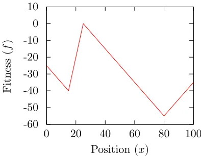
whether an algorithm can find the global optimum by either (1) escaping from the trap,

or (2) following both forks of the problem.

ffork(x) =         

       

ma(x₋xa) +mb(xa₋xb) x < xa

mb(x−xb) xa< x < xb

mc(x−xb) xb < x < xc

md(x−xc) +mc(xc−xb) x > xc

The Speciating Selection Event Algorithm: Evolutionary Computation Inspired by Darwin's Finches and Sewall Wright.

Abstract

Dedication

Biography

Acknowledgements

Table of Contents

List of Tables

List of Figures

List of Algorithms

List of Acronyms

List of Symbols

CHAPTER

1

Introduction: Evolutionary Computation

1.1

Evaluation

1.2

Encoding

1.3

Selection

1.3.1

Competition-free Selection

1.3.2

Selection with Global Competition

1.3.3

Selection with Restricted Competition

1.3.4

Other Alternatives

1.4

Variation

1.4.1

Recombination

1.4.2

Mutation

1.5

Population

1.5.1

Population Sizing and Varying

1.6

The Canonical Algorithms

CHAPTER

2

Test Problems

2.1

Ellipse

2.2

Real-Valued Trap (1-D)