Estimating Ancestral Population
Parameters
John Wakeley and Jody
Hey
Department of Biological Sciences, Rutgers University, Piscataway, New Jersey 08855-1 059 Manuscript received September 2, 1996
Accepted for publication December 6 , 1996
ABSTRACT
The expected numbers of different categories of polymorphic sites are derived for two related models of population history: the isolation model, in which an ancestral population splits into two descendents, and the size-change model, in which a single population undergoes an instantaneous change in size. For the isolation model, the observed numbers of shared, fixed, and exclusive polymorphic sites are used to estimate the relative sizes of the three populations, ancestral plus two descendent, as well as the time of the split. For the size-change model, the numbers of sites segregating at particular frequencies in the sample are used to estimate the relative sizes of the ancestral and descendent populations plus the time the change took place. Parameters are estimated by choosing values that most closely equate expectations with observations. Computer simulations show that current and historical population param- eters can be estimated accurately. The methods are applied to DNA data from two species of Drosophila and to some human mitochondrial DNA sequences.
H
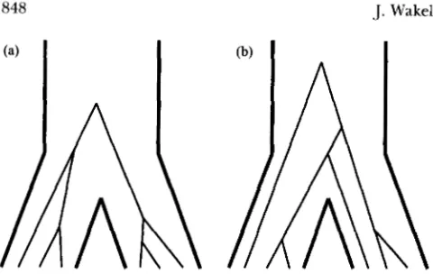
ISTORICAL events such as the formation of twospecies from a common ancestor or drastic changes in population size manifest themselves in the DNA of organisms by structuring the genealogies of nucleotide sites. Consider a situation where a single ancestral population splits into two descendent popula- tions, and after the split no genetic exchange occurs between the two. Figure 1 depicts this isolation model and shows examples of two possible genealogical histor- ies of a site in the sample. The branches in Figure 1 represent ancestral lineages of the sampled sequences. If the per-site mutation rate is small, which we will as- sume is true, then each branch presents opportunities for the creation of a particular kind of polymorphic site. When a mutation has occurred on one of these ancestral lineages, it appears as a polymorphic site that divides the sample into two groups: one that shows the ancestral nucleotide and one that shows the new, mu- tant nucleotide.
For example, a mutation on the long internal branch of the genealogy in Figure l a will divide the sample into two groups that correspond exactly to the two p o p dation samples. This type of polymorphism is com- monly referred to as a fixed difference (HEY 1991 ) . In contrast, the genealogy in Figure l b does not allow for the possibility of a fixed difference because there is no branch that divides the sample appropriately. Instead, a mutation on the smallest internal branch of that gene- alogy yields a different type of polymorphism: one that is shared by both populations. A mutation on any other branch than these two in either Figure l a or b will
Corresponding authur: j o h n Wakeley, Nelson Biological Labs, P.O. Box 1059, Rutgers University, Busch Campus, Piscataway, Nj 08855
1059. E-mail: [email protected]
produce a site that is polymorphic in only one of the two population samples. Thus, Figure 1 illustrates the relationship between population history and classes of segregating sites, as mediated through sites’ genealo- gies. If the time of separation of the two descendent populations is short, then genealogies will likely resem- ble the one in Figure l b and shared polymorphisms may appear in the data. If the time of separation is long, the most probable genealogies will, like Figure la, have an internal branch on which fixed differences can accumulate.
For any given time of separation, every possible gene- alogy will have an associated probability. However, in the absence of recombination, all sites in a particular sample will share the same genealogy. The particular one observed will be a single draw from the universe of possibilities. As single observations, individual gene- alogies are not likely to contain enough information to make accurate and general statements about popula- tion-level processes. On the other hand, if there is re- combination or if multiple loci are sampled, then differ- ent sites may have different genealogical histones. In the case of a sample from two populations, some sites’ genealogies may resemble the one in Figure l a a n d others may be like the one in Figure lb. In large data sets, many of the possible genealogies will be realized in the histories of sites in the sample and will be repre- sented in proportion to the relative likelihood of o b serving each.
A similar picture can be drawn of the sizechange model, which is like the isolation model but with only a single descendent population. Here, polymorphic sites can be partitioned according to the frequencies of mu- tant and nonmutant bases, as, for example, TAJIMA
(198913) and FU and LI (1993) have done. Again the
,J. Wakeley and J. Hey
FIGURE 1.-Two possible genealogies of a sample of three sequences from each of two isolated populations. Thick lines represent population boundaries, and thin lines trace the ancestral lineages up into the past.
numbers of each kind of polymorphic site observed in a sample of DNA will depend on the genealogies of sites, which, in turn, depend on the time and magni- tude of the change in population size. For instance, if the population has recently grown in size, sites' genealo- gies will tend to have longer terminal and shorter inter- nal branches relative to the genealogy of a sample from a constant-sized population ( SLATKIN and HUDSON 1991 )
.
This will result in an excess of sites where the mutant base is in frequency 1/
n in a sample of n se- quences and a dearth of middle-frequency polymorphic sites.We adopt general and easily interpreted versions of the isolation and size-change models. Before genera- tion 1 in the past, there was a single, panmictic popula- tion of size N A . Exactly at t , the ancestral population either split into two descendent populations (isolation model) or simply changed size ( size-change model)
.
The descendent populations are also panmictic, but in the isolation model there is no gene flow between them. The sizes of the descendent populations are Nl and N2 (isolation) orjust Nl (size-change ) , and no restrictions are put on the relative sizes of Nl , N 2 , and N , . All populations conform to the commonly used Wright- Fisher model ( FISHER 1930; WRIGHT 1931). Genera- tions are nonoverlapping and N, ,&,
and NA remain constant over time except at t , where there might be a change in population size. All variation is assumed to be neutral and mutations occur according to the infi- nite sites model with mutation rate u per sequence per generation. Four parameters, t h e n , describe the isola- tion model: 0, = 4Nlu, 0, = 4N2u, 0, = 4NAu, and r = 2ut. The size-change model is characterized by three parameters: 0 1 , 1 9 , ~ and 7 .The isolation and size-change models form the basis of many current studies in population genetics. The isolation model has been considered both as a null model of species formation (HEY 1994) and as a model of the divergence of populations (TAKAHATA and NEI 1985).
As
used here, it involves four parameters and thus represents a generalization of past implementa- tions, e.g., those of TAKAHATA and NEI ( 1985) and HUD-SON et al. ( 1987), The size-change model has been ap-
plied to recent human evolution (ROGERS and
HARPENDING 1992). However, a model of exponential growth has also been suggested ( SLATKIN and HUDSON 1991 ) and may be more realistic than the instantaneous size-change model. Clearly, both the isolation and size- change models are simple models. Whether or not they are too simple to describe the history of most popula- tions and species is an empirical question that deserves attention.
Our purpose here is to show how we can glean more information from DNA data to estimate both current and historical population parameters. This is a starting point, from which other questions might spring and be addressed, and to which other factors, such as migration and selection, might be added. We begin by deriving the expected values of the various partitions of polymor- phic sites. These then form the basis of a method of estimating the parameters of the isolation and size- change models.
THEORY AND METHODS
The segregating sites in a sample of sequences from two populations can be partitioned into four mutually exclusive categories that correspond to different aspects of genealogical history. The first comprises sites that are polymorphic in pop- ulation 1, but monomorphic in population 2 . Next are sites that are polymorphic in population 2, but monomorphic in population 1 . Call the numbers of each of these types of exclusive polymorphic sites S,, and Sm. The third are sites at which a polymorphism is shared across population bound- aries, i.e., where the same two bases appear in both popula- tions' samples. Let the number of shared polymorphic sites be called S,,. Fourth, there are sites showing fixed differences between the two populations, the number of which are re- ferred to as S,.
Segregating sites can be also classified as polymorphic in one population, either 1 or 2, regardless as to whether they are polymorphic in the other population. Call the numbers o f polymorphic sites counted in this manner S I and Si. Finally, we can simply count the total number of polymorphic sites in the entire sample, and the number of these is referred to as S. These different categories of sites are related in the following way:
s
=s,,
+
s,,
+
S,S+
s,.
( 3 )Single-population expectations: To calculate the expecta- tions of S,, , SxL, S, and S,?, we use ( 1 ) - ( 3 ) and start with the simplest case. Consider two samples of sequences taken from a single, randomly mating, diploid population of effec- tive size N . Let the numbers of sequences sampled be
TZ,
andmi. WATTEMON (1975) showed that
where 0 = 4Nu and n = n,
+
m2. In fact, Equation 4 applies to any randomly taken sample, so thatn 1 - 1 1
' I y - 1
E ( & ) = 0 7 and E ( & ) = 8
2
7 . ( 5 )Then, only one more quantity is required in order to know the expectations of all four mutually exclusive partitions of segregating sites in a single population. The expectation of S, can be derived by considering the number of sites that divide the sample into n1 and % sequences. The expected number of these is B( 1 / n1
+
1 / %) / 6, where 6 is 2, if n1 =Q and 1 otherwise (TAJIMA 1989b; FU and LI 1993; FU 1995). The chance that these n1 and % bases are distributed among the two subsamples as a fixed difference is related to the hypergeometric distribution and is just 6 / ( il ) . Thus,
is the expected number of fixed differences in a sample of n =
n1
+
% sequences from a single, randomly mating population. Then, using ( 1 ) - ( 3 ) ,L J
L J
L
are the expected numbers of polymorphisms exclusive to p o p ulations 1 and 2, and of polymorphisms shared between 1 and 2.
Two isolated populations: Under the isolation model, Equations 6-9 give the expectations of the four mutually exclusive partitions of segregating sites in the ancestral popu- lation. However, the numbers of distinct ancestors of the pres- ently sampled n1 and n, sequences, which existed at the time the two populations separated, are unknown. These numbers, called n ; and ni, must be considered random quantities that follow some probability distribution. TAKAHATA and NEI (1985) derived the following expression for the probability that, at generation t in the past, there are ni ancestors of n1
sequences sampled at the present:
if n ; = 1
In ( 10) and ( 11 ) , T I , which is equivalent to 7 / B 1 , is the time of separation measured in units of 2Nl generations. The equations for population 2 differ from these only by a change of subscripts. Thus, the probability that the ancestors of the presently sampled n, and % sequences numbered n ; and
ni at generation t is equal to Pnl,; ( 7 / B 1 ) PmJn; ( T /
e,).
The expectations of Sxl, Sx2, S,s and Scare derived by consid- ering every possible ancestral sample at time t and weighting by the probability of each. This is most clearly seen for shared polymorphic sites because these can result only from muta- tions that occurred before the time of separation of the popu- lations. The average of ( 9 ) is taken over all possible relevant ancestral sample sizes:E ( & ) = 8, p ~ l ~ ~ ( 7 / B ~ ) ~ ~ 2 ~ ~ ( 7 / B z ) I t "
n;=e a ; = 2
where n' = n ;
+
n;.Every mutation that occurs in either of the descendent populations, given that n; > 1 or
4
> 1, appears as an exclu- sive polymorphism in the data. The expected number of these in population 1 is simplyIn words, E ( Sxl after t ) is equal to the expected number of segregating sites in a sample of n1 sequences, regardless of time, minus the expected number of these that would have occurred before time t in the past. Equation 7 helps in deriv- ing the expectation of Sxl before t :
"I
E ( S X , before t ) = @ A p,,,; ( ~ / @ I ) ~ ' ~ ~ " ; ( T / B ~ )
n ; = 2 n;=1
r
/ 1 l \ lNote that in ( 14) when n; = 1 the middle term in the brackets is defined to be equal to zero. Again, the equation that applies to Sxe is obtained simply by switching subscripts. Of course,
E ( Sxl) = E ( SX, before t )
+
E( S,, after t ) and similarly forE ( Sxe), but these full equations are not reproduced here in the interest of space.
850 J. Wakeley and J. Hey
In addition, if there was only a single common ancestral se- quence of either population sample at the time the two sepa- rated, then fixed differences might have accumulated after the split. In Figure la, this is true for one population, but not the other. HEY ( 1991 ) calculated the expected length of time during which such fixed differences might have accumulated. Considering both populations, and in the notation used here, the expected number is given by
and, again, E (
4.)
= E ( Sf before t )+
E(S,
after t ) .Site frequenaes: Let zl., be the number of polymorphic sites at which the mutant base is found in i copies in the sample of nl sequences from population 1. Likewise, repre- sents mutations of size i in the sample from population 2. Using the same sort of approach, it is possible to derive the expectations of these quantities. These are especially im- portant for the size-change model because shared, fixed, and exclusive polymorphisms are defined only when there are two populations. Again, mutations can be separated into two groups: those that occurred before the population split and those that occurred after. Then, E ( zl,, before t ) is given by
E ( z l , , before t )
?*" 1
= P n + i ( ~ / O 1 )
i
P ( k - + i l n l , n : ) E ( z , , d , ( 1 7 ), , / = 2 k= 1
where P( k -+ i I n l , ni) is the probability that a mutation of
size k in the sample ni grows to size i in the sample n1 and
E ( z ~ , ~ ) is the expected number of mutations of size k in the sample n: at the moment the two populations split apart.
The expectation of z A , k is equal to O A / k ( TAJIMA 1989b; Fu
1995). P( k -+ iI nl, n;) is represented by the Polya-Eggen-
berger distribution; for example, see JOHNSON and KOTZ (1977), section 4.2. In words, P( k-+ i l nl, n;) is the probabil- ity that ( i - k ) mutant lines are added when ni lineages
become nl by the random selection and then bifurcation of lineages. It follows that
P ( k - + i l n l , n()
nl - n ; k[c--kl ( n ; - k ) [ n l - n ; - l + k l
(
i - k)
n;rn,-n:l > (18)w h e r e ~ [ ' ~ = x ( x + l ) ( x + 2 ) * * . ( x + r - l ) . The expectation of z,,? after tis calculated similarly to ( 13) : E ( after t )
and overall, i.e., E ( q t before t )
+
E ( zl,z after t ) ,Again, the expression for E( z2,* ) is gotten simply by changing subscripts. Equation 20 is the decomposition of E ( SI ) into site frequencies; E ( z l , $ ) is taken without regard to polymor- phism in population 2. Thus, ( Z O ) , when summed over all possible frequencies, i = 1 to i = n - 1, is equivalent to TAJIMA'S (1989a) Equation 9.
Of course in data, without an outgroup, we cannot distin- guish between mutations represented by i copies and those represented by nl - i copies, because we do not know which is the ancestral base. Let qt be the number of polymorphic sites with frequency i/ nl in the sample, where now i 5 nl / 2.
Then
where
S
is two if i = nl - i and one otherwise (Fu 1995).Jointly polymorphic sites can also be distinguished by their frequencies. Let zi, be the number of polymorphic sites at which the mutant nucleotide has frequency i / nl in the sam- ple from population 1 and frequencyj/ m2 in the sample from population 2. Then
where
is the probability that a mutant of size ( k ,
+
& ) / ( n ;+
n;in the-ancestral sample has kl copies in the sample n; and copies in the sample n i .
Estimating population parameters: The theory outlined here provides a framework for parameter estimation. The isolation model has four parameters and, correspondingly, we can partition the segregating sites in a sample from two populations into four mutually exclusive categories. The ex- pected values, E ( Sxl), E ( & ? ) , E ( & ) , and E ( S f ) , are given by ( 1 2 )
-
( 1 6 ) , and, although complicated, are simply func- tions of the four parameters, 01, 02, O A , and T . By equatingobserved values of S,, , Sm, SS, and Sfwith these expectations, we can solve numerically to find the values of 81, 0 2 ,
O,,
andT that most closely equate the expected and observed values. Similarly, counts of site frequency patterns can be used to estimate the parameters of the size-change model. Assume that we have taken a sample of seven sequences from a popula- tion that has undergone a rapid change in population size. There are three possible site frequency patterns and three parameters: 0, , O,, and T . A sample size of seven was chosen so that the number of possible site frequencies would be the same as the number of parameters. The expectations of q l ,
q 2 , and
vs
are given by (21 ) , so again we can equate observed and expected values and solve numerically to estimate the unknown parameters.the variance ( TAJIMA 1993; PLUZHNIKOV and DONELLY 1996; WAKELEY 1997). Thus, these methods of estimation can be used on sequences that have undergone recombination. The effect of recombination is to lower the variances of the num- bers of segregating sites, making observed values of S,, , Srz, S,, and &, or of q, , q 2 , and qs tend to be closer to their expected values. Thus recombination should improve the quality of parameter estimates ( TAJIMA 1993; PLUZHNIKOV and DONELLY 1996; WAKELEY 1997). If samples of the same size are taken from multiple loci, these methods can be used di- rectly on the combined data and are expected to perform better the more recombination occurs between loci. The methods could also easily be modified for use on multilocus samples of different sizes. When multiple loci are used, the parameters estimated are the total parameters for all loci, the sum of single-locus values.
Recombination within and among loci has a similar effect on the correlations between the various classes of polymorphic sites, ie., it decreases them. Preliminary simulations showed that strong correlations (especially between S, and Ss) associ- ated with little or no recombination significantly decreased the accuracy of these methods. As with the variances, lower correlations lead to better parameter estimates. The Drosoph- ila DNA data used below to illustrate the estimation of isolation model parameters show clear evidence of recombination both within and between loci. However, the human mitochondrial DNA data to which the size-change model is fit do not undergo recombination. In this case, we adopt another strategy for de- creasing the correlations among classes of polymorphic sites: taking subsamples of size seven from a larger data set and averaging the site frequency patterns.
SIMULATIONS AND RESULTS
Computer simulations were done to demonstrate the effectiveness of this method of parameter estimation. The isolation model was simulated using the routine “make-tree” given in HUDSON ( 1990), but with three populations (ancestral plus two descendent) , and three different population sizes, rather than one. The usual “coalescent” process proceeded independently in each of the two descendents until generation t , in the past, when the remaining sequences were united in the an- cestral population. One set of values of
01,
&, and 8, was chosen to illustrate the estimation procedure, and simulations were done over a range of the scaled time parameter, r. Five thousand replicate data sets were generated for each set of parameter values. For each data set, S X , ,Sx2,
S,T, andSf
were counted and then equated with the expectations derived above. These four equations were solved numerically using a modi- fied NEWTON-RAPHSON method; see, for example, chap- ter 9 of PRESS et al. ( 1992).
This gave estimates of 0 1 , 8 2 , B A , and r for each replicate.Preliminary simulations showed that the estimation is effective only when there is some representation in the data of the range of possible genealogies. Single genealogies do not contain enough information. Under the isolation model, for instance, without recombina- tion there can be either fixed differences or shared polymorphisms, but there can never be both. Thus, the presence of a shared polymorphism in such a sample determines that the number of fixed differences is zero.
This strong negative correlation causes the method to fail, and only disappears when there is considerable recombination or when we have samples of multiple independent loci. To insure that a number of genealo- gies would be represented in the data from each repli- cate, samples of 10 independent loci were simulated and the estimation was done only when both shared and fixed polymorphisms were observed. Within each locus no recombination was allowed.
Figure 2 shows the results of these simulations. The two descendent parameters, 81 and 82, are estimated with a fairly high degree of accuracy. To illustrate, for the case of r = 40 per locus, the standard error of 81 is only
-
10% larger than when WATTERSON’S ( 1975) estimator is used to estimate a single-population 8 from identical data, ie., 20 sequences from each of 10 loci with 8 =,20 per locus. In this same case, the standard error of d2 is only -5% larger than that of WATTERSON’S(1975) estimator. This is to be expected since, for T = 40, the chance of within population monophyly is 64% for the sample from population 1 and 81% for the sample from population
2.
As the time of separation decreases, a greater number of ancestral lineages is ex- pected, which means the data will contain less informa- tion about the descendent populations and the stan- dard error will increase.Figure 2c shows that 8, is estimated with somewhat less accuracy than 8 , and 0 2 . This is due in part to uncertainty about the configuration of the ancestral sample, but also results from the particular choice of parameters. We expect to have relatively more informa- tion about the ancestral population when the time of separation is short, but even when T = 10 per locus,
the most probable ancestral sample is ni = 3 and n; = 3. The standard error of 8, in this case, shown in Figure
2,
is about the same as when WAITERSON’S (1975) esti- mator is used with 10 sequences sampled from a single locus with 8 = 100. The time parameter, 7, is estimated quite accurately, except when the time of separation is long. In this case, r tends to be underestimated, and, correspondingly,8,
tends to be overestimated.Just one set of parameter values was chosen to illus- trate the effectiveness of using site frequencies to esti- mate 0 1 ,
e,,
and r in the size-change model. These were 81 = 21.70, 8, = 0.00, and T = 4.77 at a single locus with n = 69. These are the values estimated for one of the human mitochondrial datasets analyzed be- low. For each replicate, site frequencies were averaged over 1000 random subsamples of seven sequences from the simulated sample of 69 sequences. The average ?1 SE of the estimates of the parameters over 10,000 simulation replicates were 8, = 20.4 (229.1 )
,
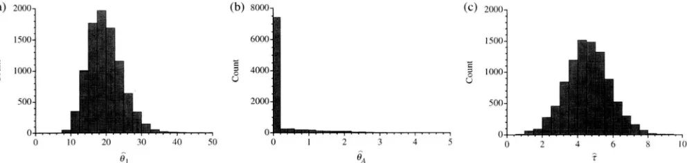
8, = 0.25 (-t0.64), and .i = 4.6 ( 5 1 . 2 ) . This level of error is higher than in estimating the parameters of the isola- tion model, probably due to the fact that here just a single locus was used. Figure 3 depicts the distributions of the estimates of the three parameters and shows thatA
852 J. Wakeley and J. Hey
(a) 300- (b) 300-
FIGLIRE 2."Simula- tion results of total pa- rameter estimates for a sample of 20 sequences from each population
when 8, = 20, 0, = 15,
100-
and 8.., = 10 per locus
50
-
50-
and data are from 10 in-dependent loci. Four
0 . I 00 1
O I O o 200 300 400 500 follows: 10, 20, 30, and values of r were used as
7 r 40 per locus. Solid black
boxes plot the means of the estimated parame-
(c) 300- (d) 300- tcrs over all replicates
that showed both shared
250- 250- and fixed polymorphic
sites. 0111 of a total of
5000 replicates, the num-
6~
150 T 150- hen of times this oc-curred were 3343, 4862,
eqml to 10, 20, 30. and 40 per locus, respectively.
07 I 0 . 1 Ran, 1 SE ofthe estimates
'"I
1
i
1
i
250-200 200-
61 150- 6 2 150-
[
4
$
$
100-
0 1 0 0 200 300 400 500
200!
i
1
1
I
200-
1 0 0 100- 3345, and 1455 for T
50 50-
0 1 0 0 200 300 400 500 0 100 200 300 400 5 0 0 over replicates.
7 r
estimates cluster mainly around the true parameter Val- lines from each species. There were a total of 56 polymor-
ues. FigureA3b shows the extreme Lshape of the distri- phisms exclusive to
D.
simulnns and 47 exclusive toD.
bution of
O,,.
m i l e the mean quoted above indicates mnun'tiann, 11 shared between the two, and six fixed dif-bias in estimating O A , fully 75% of the estimates were ferences. Thus, S . Y l = 56, &2 = 47,
&
= 11, andS,
= 6.smaller than 10"'. Table 1 shows the result3 of solving for the parameters
that give the best fit to these numbers.
From the estimates in Table 1 and assuming that
the mutation rate has remained constant over time, it
We used some previously reported DNA sequence data appears that the ancestor of
D.
simulans andD.
mauri-from two closely related species of Drosophila to illustrate tiann had an effective population size that was interme-
the estimation of Ol , 0 2 ,
O.,,,
and T in the isolation model. diate between those of its two descendents. Further, theSpecies 1 was
D.
simulnns and species 2 wasD.
mmritinna. population size ofD.
mauritinnn is estimated to be aboutThese two species separated only -770,000 years ago and threequarters that of
D.
simulnns. The two species aredata from three Xlinked loci were previously obtained. estimated to have split apart 9.0 mutational units in the
Since X-linked loci have threefourths the effective popula- past, but this is not the customary measure of time in
tion size of autosomal loci, estimates of 01,
02,
andO,,,
population genetics; time is typically measured in unitswill be correspondingly lower. KIJMAN and HEY (1992) of 2 N generations. For
D.
simulnns this is estimated assequenced 1878 bp of the pmod locus and HEY and KIL 0.60 whereas for
D.
maun'tiann it is estimated to be 0.78,M A N ( 1992) sequenced of 999 bp the m t e locus and 11 14 which reflects the difference in effective population size
bp of the yolk prokin 2 locus in the same six isofemale of these two species.
APPLICATION TO DNA DATA
(b) SW-]
6000-
-
= 4000-
8
2000-
0 I O 211 i l l 40 SO
. . .
0 I 2 3 4 5 0 2 J h x OI
6, e, r
Estimates of population parameters for D. simttlans and D. matcritiana
Parameter
(.
, o t .. I esponding estimates: total expectationsA dataset of human mitochondrial DNA serves to illustrate the use of site frequencies in estimating cur- rent us. historical population sizes. In estimating HI and
1 9 , . ~ , it is important to note that because mitochondria
are haploid and maternally inherited in humans, their effective population size is about one-fourth that of au- tosomal loci. DIRIESZO and
1471.~0s
( 1991 ) sequenced part of the control region i n 11 1 hllmans: (59 from Sar- dinia and 42 from the Middle East. They suggested that the unimodal distribution of painvise difkrences forthese populations resulted from recent growth i n popu- lation size i n both Sardinia and the Middle East. ROGERS
and H;\RI'KSDISG ( 1992) later 1 w d these distributions to estimate the ptrameters of a model of instantaneous growth identical to the present size-change model with
H I
>
H,l. They estimated that H I = li.3.5, H,, = O.fG, andT = 3.99 for S1rdina and H I = 31 17.40, H., = 0.00, and 7 = 7.54 for the Middle East ( ROGI:.RS and HARITSINSG
1992)
.
Fitting expectations, given by Equation 21above, to the averages of
v l ,
+.
andv:(
over 100,000random srdxamples of seven sequences, w e obtain H I
= 21.70, H,l = 0.00, and T = 4 . i f for Sardina and
1 9 ,
=21.94, = 0.00, and T = 831 for the Middle East. Thus, o11r analysis also supports a relatively recent and
rapid expansion for these ~o populations.
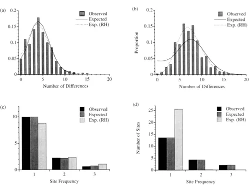
Figure 4 shows the distributions of painvise differ- ences ( a and h ) and the average site frequency counts ( c and d ) for D ~ R l ~ s z o and \VII.SOS'S ( 1991 ) Sardin- ian and Middle Eastern data. Also shown are the ex- pected distributions and collnts for each, given the different estimates made here 7)s. those of ROGERS
and HAIWESI)ISG ( 1992)
.
Figure 4a shows that, for Sardinia. both our estimates and those of Ro(;I.:Rs andSardinia Middle
East
Observed Observed
-
Expected - Expected. . .
- Exp.
(RH) . . .0.15 Exp. (RH)
8
3
.-
-
8
0.13 v
&
0.05
. I -
o
,
. ~ . ~ .
.
, , . , ,0 5 1 0 15 20 0 3 I O 15 20
Number of Differences Number of Differences
I " "
I 3
Site Frequency
1 7
-
>Site Frequency
8.54 J. Wakeley and J. Hey
HAKITNDING ( 1992) give similar predictions for the
distribution of painvise differences and that these fit
the obsened data well. Figure 4c shows that, as ex-
pected, the estimates made here provide a nearly per-
fect fit to the site frequency distribution, but ROGERS
and HAKITSDIX’S (1992) numbers fit well also. A
different situation is found for the Middle East,
shown in Figure 4, b and d. Our estimates based on
site frequencies do not reproduce the distribution of
painvise differences and ROGERS and HARPENDING’S
(1992) estimates based on the distribution of pair-
wise differences predict a very different pattern of
site frequencies than what is observed.
DISCUSSION
Polymorphic sites i n a sample of DNA sequences can be partitioned into categories that correspond to
components of genealogical history and from which
population parameters can be estimated. The meth-
ods of estimation presented here depend on a decou-
pling of different sites’ histories, so that many of the
possible genealogies are realized in the sample. For
example, the accurate estimation of
01,
0 2 ,e,,,
and 7requires that both shared and fixed differences be
observed. However, this is not possible if all sites in
the sample share the exact same history because any
single genealogy allows for the creation of only one of these two kinds of polymorphic sites. This intro-
duces a strong negative correlation between S, and
Sf
in the isolation model, which decreases only when
there is recombination in the sequences or when mul-
tiple loci are studied.
The Drosophila data analyzed above show ample evi- dence of recombination. Applying the “four gamete”
test of HUDSON and KAPIAN (1985) to the period locus
sequences, a minimum of seven and nine recombina-
tion events are inferred to have occurred in D. simulans
and
D.
nmwilinnn, respectively (KLIMAN and HEY1992). In addition, hvo other loci were used together
with pvriorl in the example above. Thus, the numbers
of polymorphic sites used in the estimation routines
probably reflect population history rather than the cor- relations imposed by particular genealogical structures. Simulations show that when this is true the resulting estimates are close to their true values.
Another method of estimating O,, and T in the isola-
tion model was developed by TAKAHATA (1986) and
extended to the case of three species by TAKAHATA et
d .
( 199.5). Those methods require multiple loci witha sample size of one from each species. This precludes
the observance of ancestral polymorphisms and serves to distinguish those methods from the one we have developed here. “ h e n species are distantly related
enough that shared polymorphisms are rare,
TAKAHA-
TA’S ( 1986) and TAKAI-IATA et nl.’s ( 1995) will be the
nwthods of choice. Of course, they will also work when
shared polymorphisms and fixed differences are both
likely to be observed, but in such cases it may be prefera-
ble to use the method developed here (provided that samples of more than one sequence are available) be-
cause it extracts the information contained i n ancestral
polymorhphisms.
When only shared polymorphisms are observed, as
will often be the case for very recently diverenged popu-
lations or species, especially when there is no recombi- nation, the following method could be used to extract information about the common ancestor, independent of the descendents. In this case, the minimum interpop
ulation pairwise differences, i x . , the smallest I<,, where
k, is the number of differences between sequence i from
population 1 and sequence j from population 2, will
give a reasonable estimate of T (TAKAHATA and NEI
1985). The estimate will, of course, be somewhat larger
than the true value of T , but the magnitude of this bias
is small when there are two or more ancestral lineages,
as required to observe shared polymorphisms. The aver-
age number of interpopulation pairwise differences,
1
”’
’5nl% , = I ; = I
dl2 =
-
It,, (24) can also be computed, and under the isolation modelthis has expectation T
+
8,,.
Then 8,, is estimated simplyby d12 - min (
Kq).
Simulations results (not shown)demonstrate that these estimators of 7 and O,.,, while
slightly biased, have very low standard errors. SAITA d
al. ( 1991 ) used min
(k,)
to estimate evolutionary ratesin Mhc loci.
The reciprocal disagreement, shown in Figure 4, be-
tween the Middle East data and the expectations for the size-change model from parameter estimates made
here using site frequencies and by ROGERS and HAR-
PENDING (1992) using pairwise differences, is interest-
ing and deserves further study. I t implies a lack of fit
between the size-change model and the Middle East- ern data. The hypervariable segment of the control
region sequenced by DIRIENZO and W I U O N ( 1991 )
0.3 Observed
Expected
0.25
c
.d 0 0.2
%
0.152
0.10.05
0
c)
L
a
0 5 10 15 20
Number of Differences
855
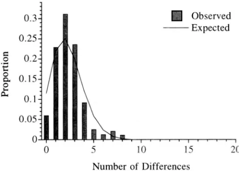
displays a great deal of variation in substitution rate among nucleotide sites (WAKELEY 1993), and this might explain the discrepancies. Figure
5
shows the result of redoing our analysis after excluding 22 sites determined to have changed more than once by the method of WAKELEY (1993). In this case, the parame- ter estimates from average site frequencies are O1 =24.46, O A = 0.00, and T = 2.46. In Figure 5, as in Figure 4c, simulations with these parameter values were used to compute the expected distribution of painvise dif- ferences. The improvement in the fit between the (new) observed distribution of pairwise differences and our expectations implies that multiple changes at some sites may explain the apparent lack of fit of the size change model. However, throwing out data (in this case 22 out of 60 polymorphic sites) is probably not the ideal approach. Better would be a full account- ing of rate variation in the development of methods similar to the ones proposed here.
Comments of two anonymous reviewers improved the manuscript. This work was supported by National Institutes of Health grant GM- 17745-01 to J.W. and National Science Foundation grant D E E 9306625 to J.H.
LITERATURE CITED
DIRIENZO, A,, and A. C. WILSON, 1991 Branching pattern in the evolutionary tree for human mitochondrial DNA. Proc. Natl. Acad. Sci. USA 8 8 1597-1601.
FISHER, R. A,, 1930 The Genetical T h e q of Natural Selection. Clarendon, Oxford.
Fu, X.-Y., 1995 Statistical properties of segregating sites. Theoret. Pop. Biol. 48: 172-197.
Fu, X.-Y., and W.-H. LI, 1993 Statistical tests of neutrality of muta- tions. Genetics 133: 693-709.
HEY, J., 1991 The structure of genealogies and the distribution of fixed differences between DNA sequences from natural popula- tions. Genetics 1 2 8 831-840.
HEY, J., 1994 Bridging phylogenetics and population genetics with gene tree models, pp. 435-499 in MolecularEcobgy andEvolution: Approaches and Applications, edited by B. SCHIERWATER, G. P. WAGNER and R. DESALLE. Birkhiuser Verlag, Basel, Switzerland. HEY, J., and R. M. KLIMAN, 1992 Population genetics and phyloge- netics of DNA sequence variation at multiple loci within the Drosophila melanogasterspecies complex. Mol. Biol. Evol. 10: 804- 822.
HUDSON, R. R., 1990 Gene genealogies and the coalescent process, pp. 1-44 in Ox ford Surueys in Evolutionaq Biology, Vol. 7, edited by D. J. FUTUYMA and J. ANTONOVICS. Oxford University Press, Oxford.
HUDSON, R. R., and N. L. KAPIAN, 1985 Statistical properties of the number of recombination events in the histoty of a sample of
DNA sequences. Genetics 11 1: 147- 164.
HUDSON, R. R., M. KREITMAN and M. AGUADE, 1987 A test of neutral molecular evolution based on nucleotide data. Genetics 116:
JOHNSON, N. L., and S. KOTZ, 1977 Urn Mu&& and 7%rirApjJ/icalion. Wiley, New York.
KLIMAN, R. M., and J. HEY, 1992 DNA sequence variation at the period locus within and among species of the Drosophila melanogar- ter complex. Genetics 133: 375-387.
PLUZHNIKOV, A., and P. DONELI.Y, 1996 Optimal sequencing strate- gies for surveying molecular genetic diversity. Genrtics 1 4 4
PRESS, W. H., S. A. TEUKOISKY, W. T. VETI-ERI.ING and B. P. FI.ANNE.RI', 1992 N u m ' c a l Recipes in C: Thr Art of S r i m l i j i c Cornpuling Cam- bridge University Press, Cambridge.
ROGERS, A. R., and H. HARPENDING, 1992 Populations growth makes waves in the distribution of painvise differences. Mol. Riol. Evol.
SATTA, Y., N. TAKAHATA,
c.
SCHONBACI-I, J. GUTKNECHT and J . KI.EIN,1991 Calibrating evolutionary rates at major histocompatibility complex loci, pp. 51 -62 in MolecularEvolution ofthe Hzstocomnpati-
bility Complex Loci, edited by J. K L E I N and D. K L E I N . Springer- Verlag, Berlin.
SLATKIN, M., and R. R. HUDSON, 1991 Painvise comparisons of mito- chondrial DNA sequences in stable and exponentially growing populations. Genetics 129: 555-562.
TAJIMA, F., 1989a The effect of change in population size on DNA polymorphism. Genetics 123: 597-601.
TAJIMA, F., 1989b Statistical method for testing the neutral mutation hypothesis by DNA polymorphism. Genetics 123: 585-595. TAJIMA, F., 1993 Measurement of DNA polymorphism, pp. 37-59
in Mechanisms of Molecular Evolution, edited by N. TAKAHATA and A. G . CLARK. Sinauer Associates, Sunderland, MA.
TAKAHATA, N., 1986 An attempt to estimate the effective size o f
the ancestral species common to two extant species from which homologous genes are sequenced. Genet. Res. Camb. 48: 187-
190.
TAKAHATA, N., and M. NEI, 1985 Gene genealogy and variance of interpopulational nucleotide differences. Genetics 110: 325-
344.
TAKAHATA, N., Y. SATI-A and J. KI.EIN, 1995 Divergence time and population size in the lineage leading to modern humans. Theoret. Pop. Biol. 48: 198-221.
WAKEL~, J., 1993 Substitution rate variation among sites in hyperva- riable region 1 of human mitochondrial DNA.J. M o l . Evol. 37:
WAKELEI', J., 1997 Using the variance of painvise differences to esti- mate the recombination rate. Genet. Res. Camb. (in press). WATTERSON, G . A., 1975 On the number of segregating sites in ge-
netical models without recombination. Theoret. Pop. Riol. 7:
WRIGHT, S., 1931 Evolution in Mendelian populations. C.enetics 16:
153-159.
1247-1262.
9: 552-569.
613-623.
256-276.
97- 159.