Transactions of the 17th International Conference on Structural Mechanics in Reactor Technology (SMiRT 17)
Prague, Czech Republic, August 17 –22, 2003
Paper # K02-2
SEISMIC SAFETY ASSESSMENT OF NUCLEAR FACILITIES OTHER
THAN NPPS
Ovidiu Coman1), Andreea Dragomirescu1), Florin Kope1), Nicolae Zemtev1)
1)
Stevenson and Associates, Ltd., Romania
ABSTRACT
Many research nuclear facilities are much simpler as compared with a Nuclear Power Plant (NPP) and the accident scenarios corresponding to an external initiating events and the relevant shutdown paths are much easier to be identified. Therefore, simpler methods than an EE-PSA can be often involved in the evaluation of the overall risk associated to such nuclear facilities in respect to External Event Hazards.
KEY WORDS: PERFORMANCE GOAL, EXTERNAL EVENT HAZARD, FRAGILITY, SEISMIC RISK,
DAMAGE STATE, CUTSETS
INTRODUCTION
The External Event Hazards (EEH) considered for safety assessment of nuclear facilities should be evaluated on a probabilistic basis. The frequency of occurrence of the parameters describing the external hazard severity (such as earthquake ground acceleration, wind speed, or water elevation) is estimated by probabilistic methods. Common frequency statistics employed for rare events such as EE hazards include return period and annual probability of exceedance.
Return period is the average time between consecutive events of the same or greater severity (for example, earthquakes with maximum ground acceleration of 0.1g or greater). It must be emphasized that the return period is only an average duration between events and should not be construed as the actual time between occurrences, which would be highly variable. A given event of return period, T, is equally likely to occur any year, thus the probability of that event being exceeded in any one year is 1/T. The annual probability of exceedance, “p”, of an event is the reciprocal of the return period of that event (i.e., p = 1/T).
Performance Goal is the annual probability of exceedance of acceptable behavior limits used as a target to develop EEH design and evaluation criteria. Goals for Structures, Systems and Components (SSCs) performance during natural phenomena hazards have been selected and expressed in terms of annual probability of exceedance. Numerical values of annual probabilities of exceedance for performance goals depend on Structures Systems and Components (SSCs) safety classification.
Acceptable behavior limits considered in the performance goals also depend on the SSCs characteristics. For example, the acceptable behavior limits for normal use SSCs is major damage but limited in extent to below that at which occupants are endangered. However, the acceptable behavior limits for safety classified SSCs is lesser damage such that the facility can perform its function. Performance goal probability values apply to each Natural Phenomena Hazard (NPH) individually.
The proposed approach may be used in two steps of the whole process:
1. In the definition of the site and design approach in relation to the performance goal. 2. In the final safety evaluation at the end of the design/qualification process
These criteria also employ a graded approach to ensure that the level of conservatism and rigor in design/evaluation is appropriate for facility characteristics such as importance, hazards to people on and off site, and threat to the environment. For each natural phenomena hazard covered, these criteria consist of the following:
1. Performance categories and target performance goals
2. Specified probability levels from which natural phenomena hazard loading on structures, equipment, and systems is developed.
3. Design and evaluation procedures to evaluate response to EEH loads and criteria to assess whether or not computed response is permissible
Issues 2 and 3 are correlated and there are different possible combinations of responses to these two issues that can be used to achieve the target goal.
The Damage State Risk and/or calculation of the Safety Margin in respect to the Performance Goal should be assessed based on Safety Analysis. The general EEH safety analysis should address the followings:
- Site dependent Median EE Hazard definition in terms of annual frequency of exceedance/occurrence. - Evaluation of the design/evaluation demand associated to the EEH.
- Evaluation of the damage states or success paths associates to each EEH.
- Evaluation or calculation of the facility response, dominant failure modes and fragility.
- Damage state Risk (PF) quantification and margin evaluation in respect to the performance goal for each
EEH included into design basis.
- Evaluation of the radiological consequences.
- Review of the EEH design basis adequacy (if required).
PRELIMINARY ESTIMATION OF THE HAZARD LEVEL AND DESIGN TARGET CONSISTENT TO THE PERFORMANCE GOAL
Based on the performance goal the answers to the following questions should be provided:
1. What EE hazard demand should be selected for the design/re-evaluation process in relation to the performance goal?
2. What deterministic EEH design/evaluation criteria should be selected, in relation to the EEH demand level, will reasonably achieve the performance goal defined in terms of a target annual probability of unacceptable performance?
Fragility of a SSC is defined as conditional probability of failure (unacceptable performance) versus hazard parameter. For convenience it is acceptable to assume that failure is lognormal distributed in respect to the median capacity value. The median fragility function is defined by the median capacity value C50% and the total variability β.
The unacceptable performance or the probability of failure PF is the result of the convolution of the median
hazard curve and median fragility:
da da dP ) a ( H P
0
a / F F
∫
∞
= (1)
The solution of Eq.1 depends of how the hazard and fragility are defined. If EEH - demand intensity cannot be described by a continues function, and the hazard is defined by a single value describing the EE frequency of occurrence of the event with postulated intensity parameters (aircraft crash, explosions, etc.) Eq.1 becomes:
PF = Hazard-Level x Probability of Failure (2)
Eq. 1 could be used to check if the EE Hazard and fragility is consistent to the performance goal. It means that the calculated total probability of failure PF corresponding to an accident sequence (damage state) as result to the EEH
induced loads is less than the performance goal:
PF≤ Performance goal (3)
Design rules ensure that for a given EEH demand loading any SSC designed based on such rules, will have the median estimated failure less or equal to 1% for nuclear codes and less or equal to 10% for industrial codes. Recommended values for Hazard Level and Target Fragility (function of the selected codes) are presented in Table 1.
Table 1. Recommended values for Hazard Level and Target Fragility
Performance Goal Hazard Level Target Fragility Design rules
10-6 10-4 – 10-5 10-2 –10-3 Nuclear codes
10-5 10-3 – 10-4 10-1 – 10-2 Industrial codes +
additional requirements
10-5 10-2 –10-3 10-2 –10-3 Nuclear codes
10-4 10-3 10-1 –10-2 Industrial codes +
additional requirements
10-4 10-2-10-3 10-2 – 10-3 Nuclear codes
Note:
The shaded row corresponds to the NPP facilities.
Additional requirements may supplement Industrial Codes provisions in order to achieve the required Target Fragility.
The Target Fragility can be expressed in median capacity C50% or HCLPF capacity and total variability
The Design Base (DB)-EEH demand loading is given by the Hazard Function and selected hazard level. For the selected DB-EEH demand loading the margin against failure and appropriate design rules can be selected based on the associated Target Fragility.
In other words is required to evaluate the EE-Hazards and associated Target Fragilities that convolved together (equation 1) gives the total probability of failure that must be less then to the Performance Goal. On such basis the hazard level end the design criteria can be defined before the design process is started.
FINAL EVALUATION OF THE PLANT SAFETY
After the design process is finished the performance goal shall be evaluated and documented in the Safety Analysis Report. At the end of the design process EE-Hazards considered into design shall be available. The RR performance evaluation in relation to EE-Hazards includes the following steps:
Perform selection of the success path and/or accident sequences to be considered in the safety analysis (SSC list).
Evaluate individual SSCs fragility based on design documentation. A simplified evaluation can be conducted based on design review and design codes analysis. The outcome of this evaluation is the median capacity and associated variability. The capacity variability can be evaluated using generic data and engineering judgement. The median capacity and total variability define the fragility function of individual SSCs.
Combining individual SSCE fragilities, using logic expressions of success paths or damage state cutsets, is obtained the nuclear facility fragility. Also the weak links could be identified and some design changes could be recommended.
Use Equation (1) to calculate the total failure probability and compare PF with the Performance Goal
(check Equation 3).
Also the above steps can be used to evaluate existing nuclear facility. In such cases detailed inspection shall be conducted to collect as-built, as operated and as is information for the SSCs.
SIMPLIFIED APPROACH FOR SEISMIC RISK ASSESSMENT
The Simplified Hybrid Method is proposed to be used for seismic safety evaluation of existing nuclear facilities or seismic design review of the new ones. This method is effective especially for nuclear facilities where the success path or the plant damage state cutset can be determined with less effort as for a NPP.
The Hybrid Method is a combination between the Seismic Probabilistic Risk Assessment (SPRA) and Seismic Margin Assessment (SMA) Methods using the advantage of SPRA with the simplification of the SMA. The background of the Hybrid Method is described in [1].
The main steps are as following:
a. Simplified Mean Hazard curve estimation
b. Primary and secondary Success Paths or facility Damage State cutsets selection (SSC list of items to be qualified against EEH). Seismic Walkdown and CDFM-HLCPF calculation for the selected SSCs.
c. Evaluation of variability parameters β and calculation of the plant HCLPF or damage state fragility d. Estimation of the Damage State risk PF
a) Simplified Hazard Estimation
The seismic Hazard curves may be assumed close to linear when plotted on a log scale. Thus over at least any ten-fold difference in exceedance frequencies such hazard curves may be approximated by:
H
K Ia K ) a (
K = − (4)
where K(a) is the annual frequency of exceedance of ground motion level “a”, KI is the appropriate constant, and KH is a
slope parameter defined by:
) A log(
1 K
R
H= (5)
in which AR is the ratio of ground motions corresponding to a ten-fold reduction in exceedance frequency. AR typical
ranges between 2 and 5.
b) HCLPF Evaluation
c) Variability Estimation
For structures and major passive mechanical components mounted on the ground or low elevations within structures, β typically range is 0.3 to 0.5. For active components mounted at high elevations in structures the typical β range is 0.4 to 0.6. Note that overestimating β is un-conservative because it increases C50%. Limited calculations or
published data for similar components can be used for β estimation if as-built and as-operated conditions comply with the caveats listed in [2 – 3].
d) Determine SSC Seismic Risk PF
The relationship between CDFM-HCLPF capacity (CCDFM) and median capacity (C50%) is:
C50% = CCDFM e 2.326β (6)
Estimate 10% conditional probability of failure capacity C10% from:
C10% = Fβ CHCLPF (7)
Fβ = e1.044β
Determine hazard exceedance frequency H10% that corresponds to C10% from hazard curve.
If the fragility curve PF/a is log-normally distributed and hazard curve is defined by equation (1), a rigorous
closed-form solution exists for the seismic risk equation:
da da dP ) a ( H P 0 a / F F
∫
∞ = (8)
α −
=HF e
P KH
% 50
F (9)
H % 50 % 50 C C
F = (10)
2 ) K ( Hβ 2 =
α (11)
where H is any reference exceedance frequency, CH is the ground motion level that corresponds to this exceedance
frequency H from the seismic hazard curve, C50% is the median fragility, and β is the logarithmic standard deviation of
the fragility. Next a specific hazard exceedance frequency H10% is substituted for H, where H10% is defined at the ground
motion corresponding to 10% conditional probability of failure. Thus:
β
= = 1.282
% 10 % 50 % 50 e C C
F (12)
from which: β − = h % 10 F/H e
P (13)
hβ = 1.282(KHβ) – 0.5(KHβ)2 (14)
) ) K ( 5 . 0 K ( 282 . 1 ( % 10 F 2 H H e H
P = − β− β (15)
Over the most common ARrange, the following relationship for the PF is obtained:
PF = 0.5 H10% (16)
For β = 0.4 equation (12) can be used for AR from 1.6 to 5. However, this range should cover essentially any
hazard curve of interest.
QuickSFP COMPUTER CODE USED TO ENHANCE THE SIMPLIFIED APPROACH
A Windows based computer code named QuickSFP has been developed as an useful tool to be used for seismic risk quantification. QuickSFP is able to solve the following calculations:
Generate fragility curve based on fragility parameters Am and β
Extract data from fragility curve: Am, HCLPF, 10% capacity or conditional failure probability for
Calculate convolution integral defined in equation (8) for any shape of hazard curve (truncation limits are user defined)
Combine a set of fragility curves using a Boolean expression that defines a damage state cutsets (solve equations 17 and 18).
ILLUSTRATIVE EXAMPLE
Assuming that for items A,B,C,D,E and F the HCLPF was determined using “CDFM Method” as described in [2-3]. Associated variability β values have been selected according to Hybrid Method [1]. For each item the median capacity Am is calculated using HCLPF and associated β values.
The hazard curve is selected with equations 4 and 5 for the following parameters: AR= 2
KH = 1.0/Log(AR) = 3.32
KI = 4.78x10⁻⁶
K(a)= 4.78x10⁻⁶ x a-KH
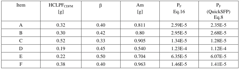
Table 2 presents Total Probability of Failure PF calculated using simplified method (Eq. 16) and QuickSFP
(Eq.8) assuming that for the given SSC items A, B, C, D, E and F the CCDFM is calculated using SMA method and then
the variability values were estimated based on engineering judgment and available published data.
Table 2. Example of calculation of Pf for individual components
Item HCLPFCDFM
[g]
β Am
[g]
PF
Eq.16
PF
(QuickSFP)
Eq.8
A 0.32 0.40 0.811 2.59E-5 2.35E-5
B 0.30 0.42 0.80 2.95E-5 2.68E-5
C 0.52 0.33 0.905 1.34E-5 1.28E-5
D 0.19 0.45 0.540 1.23E-4 1.12E-4
E 0.22 0.50 0.704 6.35E-5 6.07E-5
F 0.38 0.40 0.963 1.46E-5 1.41E-5
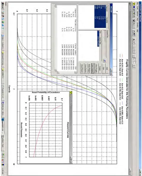
For this example can be observed a very good agreement between simplified method (Eq. 16) and accurate method (QuickSFP – Eq.8). Figures 1-1 shows few screenshots of QuickSFP containing results of the illustrative example.
Estimation of the overall probability of failure of the Facility Using the Simplified Hybrid Method
Assuming that two success paths SP1 and SP2 have been evaluated using CDFM, the damage state (DS) will occur when success paths (SP1)AND(SP2) both fail.
2 SP 1 SP
DS= I
F E D 2 SP
C B A 1 SP
U U
U U
= =
(17)
PF(DS) = PF(SP1)PF(SP2)
PF(SP1)= PF(A) + (1-PF(A))[PF(B)+(1-PF(B))PF(C)] (18)
PF(SP2)= PF(D) + (1-PF(D))[PF(E)+(1-PF(E))PF(F)]
Table 2: Report Generated by QuickSFP V2.0 produce the following results
Description Capacity Variability Expression Combined
Capacity
Combined Variability
A 0.811 0.40 SP1=A+B+C 0.610 0.316
B 0.800 0.42 SP2=D+E+F 0.458 0.391
C 0.905 0.33 DS=SP*SP2 0.653 0.262
D 0.540 0.45 - - -
E 0.704 0.50 - - -
F 0.963 0.40 - - -
Eq.17-18 shows how the individual component fragilities are combined to obtain plant damage state fragility using plant damage state cutset. The above calculations have to be done for at least 10-20 acceleration values within the acceleration range of interest.
Because of the convolution, the Damage State fragility curve has lower β than the individual component fragility curves. It is recommended that β=0.3 be used for the damage State variability.
FINAL REMARKS
The Simplified Hybrid Method is proposed to be used for seismic safety evaluation of existing nuclear facilities or seismic design review of the new ones. This method is effective especially for nuclear facilities where the success path or the plant damage state cutset can be determined with less effort as for a NPP.
The presented approach can be used for either screening in case of EE-PRA or seismic risk evaluation of nuclear research facilities. QuickSFP represents a very effective and useful tool that facilitates all analytical calculations with high accuracy.
REFERENCES
1. R.P Kennedy in “Overview of Methods for Seismic PRA and Margin Analysis Including Recent Innovations”, 1998.
2. EPRI NP-6041, “A Methodology for Assessment of Nuclear Power Plant Seismic Margin”, Electric Power Research Institute, October 1988.
3. DOE/EH-0545, Seismic Evaluation Procedure for US Department of Energy Facilities, U.S. Department of Energy, March 1977.