Estimating effective population size or mutation rate using the frequencies of mutations of various classes in a sample of DNA sequences.

(1)

Copyright 0 1994 by the Genetics Society of America

Estimating Effective Population Size

or Mutation Rate Using the Frequencies of

Mutations of

Various

Classes

in

a Sample of DNA Sequences

Yun-xin

FU

Center f o r Demographic and Population Genetics, University of Texas, Houston, Texas 77225

Manuscript received February 18, 1994

Accepted for publication August 27, 1994

that

6,

is a:ery efficient estimator.

A“

important parameter in studying the evolution of a DNA region (locus) of a population is 8 = 4Np

where N is the effective size of the population and

p

is the mutation rate per sequence per generation. From the value of 8, the effective population size N can be obtained if the mutation rate

p

is known or vice versa. Until recently inferences about 8 have been based largely on two quantities. One is the sequence diversity T, which is the average number of nucleotide differences per pair of sequences; the other is the number K of segregating sites (polymorphic sites). These two quantities lead to respectively TAJIMA’S estimate .ir of 8 and WATTEMON’S estimate

K

of 8 as follows

+ = T K =

wan

where

1 1

a n = l + - +

. . . + -

2

n - 1 (1)

and n is the sample size. Although the computations of these two estimators are easy, they are not very efficient estimators, in particular, the variance of .ir does not di- minish with increasing sample size. The inefficiency of these estimators and the surging of DNA polymorphism data have been stimulating the development of new methods of estimating 8 that make better use of the information in a sample. Phylogenetic information are very useful in developing more accurate estimators ( F E L S E N ~ I N 1992; FU 1994a). For example,

Fu

(1994a) showed that a phylogenetic estimator has a variance close to the minimum

Genetics 138 1375-1386 (December, 1994)

ABSTRACT

Mutations resulting in segregating sites of a sample of DNA sequences can be classified by size and type and the frequencies of mutations of different sizes and types can be inferred from the sample. A framework for estimating the essential parameter 8 = 4Nu utilizing the frequencies of mutations of various sizes and types is developed in this paper, where N is the effective size of a population and p is mutation rate per sequence per generation. The framework is a combination of coalescent theory, general linear model and Monte-Carlo integration, which leads to two new estimators

6,

and

6,

as well as a general Watterson’s estimator

6,

and a general Tajima’s estimator

6,.

The greatest strength of the framework is that it can be used under a variety of population models. The properties of the framework and the four estimators

bK,

e,,,

6,

and

6,

are investigated under three important population models: the neutral Wright-Fisher model, the neutral model with recombination and the neutral Wright’s finite-islands model. Under all these models, it is shown that

6,

is the best estimator among the four even when recombination rate or migration rate has to be estimated. Under the neutral Wright-Fisher model, it is shown that the new estimator

6 ,

has avariance close to alower bound ofvariances of all unbiased estimators of Owhich suggests

variances of all possible unbiased estimators of 8 under the neutral Wright-Fisher model. That is, the population under study evolves according to the Wright-Fisher model, all mutations are selectively neutral and there is not recombination and no population subdivision.

Natural populations are usually more complex than described by the neutral Wright-Fisher model. For example, they are often subdivided into small local populations with migrations among them; an autosomal DNA region studied may be very large or consist of several separate regions so that recombinations cannot be neglected; some mutations may not be neutral or mutation rates for different region of a locus may differ. Estimat- ing 8 under models other than the neutral Wright-Fisher model is often necessary for detailed analysis of polymorphism data. Although Watterson’s estimator

K

and TAJIMA’S estimator .ir can be modified to provide estimate of 8 under various models, they are likely inefficient as they are under the neutral Wright-Fisher model. On the other hand, phylogenetic methods such as Fu (1994a) and FEUENSTEIN (1992) are difficult to be extended because they require detailed properties of the branchs of a genealogy which are poorly understood under other models. In this paper, I present a framework for estimating 8 which is not only very efficient but can be used under a variety of

(2)

Y.-X. FU

where [n/2] denotes the largest integer contained in n/2 and the i-th element q i of r) is given by

FIGURE 1 .-The variants of mutations in a genealogy where each 0 represents a mutation.

FREQUENCIES OF MUTATIONS OF VARIOUS CLASSES

Consider a random sample of n sequences from a population. Corresponding to each homologous site of the sequences, there is a genealogy connecting the n sequences (nucleotides) to their most recent common ancestor and the genealogy consists of

2(

n - 1) branches. A branch is said to be size i if exactly i sequences in the sample are descendents of the branch. A mutation occurred in a branch of size i is said to be of size i or an ;mutation. Therefore, mutations leading to segregating sites in a sample can be classified into n - 1 sizes. An il- lustration of the definition is given in Figure l.

Let

5,

be the summation of i-mutations over all the sites and be a vector given by

where T stands for transpose. The vector

&

is a primary source of information that will be utilized in this study to estimate 8. When the infinite-sites model is assumed and an outgroup sequence is available, the value of &can be inferred directly from the sequences of a sample. This is because that a mutation results in a segregating site of two segregating nucleotides and the nucleotide that is not the same as that of the outgroup sequence must be the size of the mutation, otherwise it will contradicts with the infinite-sites model. However, when the infinite-sites model does not hold and there is no outgroup sequence available, the value of

&

has to be inferred by recon- structing a genealogy of the sample; when the length of sequences are not sufficiently long or there are recombinations the inferred value of

&

will often contain er- rors. Although we wish to address all important issues related to the estimation of 8, we shall assume as an initial investigation that the value of

5:

is known for a given sample.

Another vector of information that will be utilized to estimate 8 is

where 8i,n-z is the Kronecker delta, i e . , it is equal to 1 if i = n - i and 0 otherwise. Under the infinite-sites

model, q, is simply the number of such segregating sites at which the frequencies of the two segregating nucleotides are i and n - i(i c n - i) respectively. Such a segregating site is said to be of type i or i-segregating site. We thus call qi the frequency of i-segregating sites. It is easy to see that when the infinite-sites model holds the value of r) can be obtained directly from a sample with-

out the help of an outgroup sequence. Because of this reason, it is easier to use an estimator based on r) than an estimator based on

g,

although the former is inferior to the latter, as shall be demonstrated later.

BEST LINEAR ESTIMATORS OF

e

FROM

6

AND 1

Because the number of segregating site K is equal to

5,

+

. . .

+5,-

I and q1

+

. . .

+q(n/21, WATTERSON’S esti-

mator

K

can be written as

where a, is given by (1). Therefore, a i s a linear function of

el,

.

. .

,

or a linear function of ql,

. . .

,

q n I 2 ] . Since

a mutation of size i is counted in i( n - i) painvise comparisons, TAJIMA’S estimator .ir can be written as

which is also linear function of

tl,

. . .

, ( n - l , or ql,

. . .

,

q[n/21. One common feature of these linear estimators is that their coefficients, that is l / a n ,

. . .

,

l/a, for Rand 2i(n - i ) / n ( n - l ) , ( i = 1,

. . .

, n - 1) for

?r,

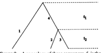
are predetermined constants. A linear estimator with predetermined Coefficients is not in general a best linear estimator. To demonstrate this, we consider a sample of only three sequences. There is only one topology for three sequences (Figure 2) and

&

= (

tl,

&) where

5,

is the sum of the numbers of mutations in all the three external branches and

5,

is the number of mutations in the internal branch. From KINGMAN’S (1982a,b) coales-

cent theory, it is easy to show [for example, FU and LI (1993b) that

~ ( 5 ~ )

= 8 E([,) =

Var(el) = 8

+

1 / O P Var(6,) = % 8

+ %e2

(3)

Estimation of Mutation Rate 1377

FIGURE 2.-A genealogy of three sequences.

6,

is the sum of the numbers of mutations in branch 1 , 2 and 3 while

6,

is the number of mutations in branch 4. See texts for the explanation of t , and t2.

Consider the following linear function of

t1

and

t2

f

= at1

+

bt2

(7)

In order for f to be an unbiased estimator of 8, it must satisfy

~ ( f )

=

ae

+

(b12)e =

e

Therefore, b =

2 (

1

-

a ) . Substituting

2 (

1 - a) for b in

(7),

we obtain the variance off as

Var(f) = a2Var(J)

+

4(1

-

a)Var(&)

+

4 4

-

a)c=ov(J,

X )

= [a2

+

2(1

- a)2]e

+

(1 - a)2]e2

It is easy to show that the value of a for the most efficient estimator, that is, the one with smallest variance, must be

( 4

+

8)/(6

+

e).

Therefore,

is the best linear unbiased estimator of 8 and the coefficients off are not predetermined. Equation 8 suggests that to have an optimal estimating scheme, we should give more weight to

t1

than to

t2

when there are many segregating sites in a sample (indicating that 8 is large) and we should give about equal weights to both

t1

and

5,

when there are few segregating sites (indicating that

0 is small). Nevertheless, we should not fix the coefficients in advance.

Similar analyses can be made for samples of more than three sequences and a general framework by Fu (1994a)

can be applied. The framework was developed for a vector of variables whose means are linear functions of 8

and variances and covariances are quadratic functions of

8. In next section, we shall show that

E(&) = ea (9)

Var(&) = OD,

+

028 (10)

where (Y = ( a l ,

. .

.

,

a n - l ) ; D, = diag(a,,

. . .

,

a n - l ) ,

i.e., a matrix whose diagonal elements are a,,

. . .

,

an-l

and all non-diagonal elements are zero, and

8

= {uv},

i , j = 1,

.

. .

,

n - 1; ai and uv are all constants inde-

pendent of 8 once the model is given. With some modi- fications of the notation in Fu (1994a), we have that the best linear unbiased estimator of 8 from

5

is given by

However, Equation 11 does not provide a direct estimate of 8 because its computation requires the value of 8 which is unknown. The problem can be circum- vented by the following iteration procedure. Define a series

and assign an arbitrary non-negative value to

e,,.

Then the limit

6,

of the series is taken as our estimate of

e.

hr

will be referred to as the BLUE (best linear unbiased estimator) of 8 from

g

and the estimation procedure as the BLUE procedure, though strictly speaking the estimator is not a linear function in

5

because of the iteration.

From the definition of q and Equations 9 and 10, it is simple to see that

E ( q ) =

ea

(13)

Var(q) =

8D,

+

02r (14)

where D, = diag(P,,

. . .

,

Pcn,21),

I'

= {yv] and

The BLUE

dq

of 8 from q is the limit of the series

and 0, can be any non-negative value. From (9), we have that

Therefore we define a general WAITERSON estimator

6,

and a general TAJIMA estimator

6,

as

e,

=

-

a n

K

I:

ai

Under the neutral Wright-Fisher model we have that

(4)

When 8 is close to zero, it is easy to see from ( 1 1 ) or

(12) that

It thus follows that when 8 is small, the general WATTERSON estimator is approximately the best linear estimator of 8.

Treating the vector of the coefficients of

8,

as a vector of constants as did in

Fu

(1994a), we have that

Var(6,) = a,@

+

b,O2

where a, = u%,u and b, =

u'xu.

It is easy to see that a nearly unbiased estimate of the variance of

6,

is

Similarly, a nearly unbiased estimate of the variance of

8,

is given by

v,

=

a,e,

..

+

- a$,

1

+

b,

where a, = v?,v, b, = v T v and v is the vector of the coefficients of 8, given by

ESTIMATION OF THE MEAN AND VARIANCE OF

6

AND 9

Consider a sample of n sequences. The time interval between the moment at which the sample is taken and the time representing the most recent common ancestor of the n sequences can be divided to a number of periods by the events occurred. In this paper, we mean, by an event, a coalescence, a recombination or a migration, but not a mutation. For convenience of notations, we treat the m e ment at which the sample is taken as

an

event. Let the events be numbered according to their orders of occur- rence and tk be the time length (in terms of the number of generations) between the kth event and

( k

+

1)th event. Under the neutral Wright-Fisher model, there are only coalescent events, so tk represents the time length for the period during which the sample has k

+ 1

ancestral sequences; therefore tk is a ( k

+

l)-coalescent time.

Suppose there are in total L sites in each sequence. Each site can be regarded as a locus and there is a genealogy for each site which connects the n nucleotides at the site to their most recent common ancestor. Consider the genealogy of the Zth site. We can see that the time length of a branch of the genealogy must be of the form

t i + . . . + %

where i is the number of the event after which the branch starts and j is the number of the event at which the branch ends. For the genealogy of lth site, the length I ( a ) of the

branchs of sue k is given by

1p = sjf,)t,

+

. . .

+

sgt,

where s 6 is an index variable representing the number of times ti appears in the time lengths of branchs of size k; p

is the total number of events. The average time length of branches of size k over all sites is therefore

1 1 I-

lk = -

x

I f ) =

C

sbti where ski =

C

s!).

L

1= t

When there is no recombination, all the L genealogies are the same and consequently s,, = sg) =

. . .

=

sti.

For example we have for the genealogy in Figure 2 that s12 = 3,

sll = 1, p2 = 0 and +1 = 1.

Because p is defined as the mutation rate per sequence per generation, the mutation rate per site per generation is therefore p/L. Assume that the number of mutations in a branch of the genealogy of a site is a Poisson variable with parameter Zp/Lwhere lis the length of the branch. Then the number of k-mutations in all the L genealogies is a Poisson variable with parameter ( p / L )

8;)

= lkp. In other words, we assume that

(5)

20

50

Estimation of Mutation Rate 1379

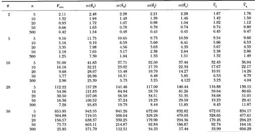
TABLE 1

Variances of four estimators under the neutral Wright-Fisher model

e

n ‘tin svce,, S U ( e , ) s v ( Q 4 e , )

vs

vq

2 5 2.11 2.48 2.28 2.21 2.28 1.87 1.76

10 1.32 1.94 1.48 1.39 1.46 1.42 1.50

20 0.93 1.72 1.07 0.98 1.04 1.02 1.12

50 0.66 1.63 0.78 0.70 0.74 0.74 0.80

300 0.42 1.54 0.48 0.43 0.45 0.45 0.47

5 5 9.16 11.75 10.65 9.73 10.59 9.54 9.60

10 5.16 9.10 6.59 5.60 6.41 5.66 6.53

20 3.35 7.98 4.56 3.63 4.33 3.67 4.33

50 2.18 7.65 3.17 2.38 2.84 2.38 2.86

300 1.25 7.30 1.84 1.33 1.51 1.32 1.49

10 5 31.00 41.83 37.71 32.50 37.44 32.43 36.04

10 16.16 32.21 23.02 17.70 22.33 17.67 22.17

20 9.68 28.67 15.48 10.79 14.27 10.91 14.26

50 5.77 26.96 10.31 6.48 5.85 6.53 8.79

300 2.96 25.39 5.73 3.25 4.122 3.23 4.04

5 112.22 157.28 141.46 117.00 140.44 116.88 139.15

10 54.96 121.83 84.94 59.79 81.26 59.64 80.65

20 30.50 107.08 56.58 34.51 51.35 34.68 51.01

50 16.38 100.52 37.24 19.23 29.58 19.23 29.41

300 7.28 95.83 19.79 8.44 11.85 8.43 11.87

5 655.95 943.55 841.26 672.60 832.82 672.01 834.17

10 304.88 719.55 500.64 329.28 479.03 328.65 477.61

20 156.57 638.37 330.25 179.90 294.36 179.45 294.23

50 73.73 603.1 1 214.87 92.84 166.87 92.74 164.16

300 25.85 571.70 112.51 34.25 57.44 33.99 056.29

Note: Results are based on 50,000 simulated samples for each combination of 0 and n. su, sampling variance.

ve

and

vq

are, respectively, the mean of Vs given by Equation 19 and the mean of V, given by Equation 20.

Suppose there are in total T genealogies for a sample of n sequences and let wlk), be the wi,

4v

defined above for genealogy k and

p ,

be the probability of o b serving genealogy k. Define

T

a, =

x

W(rk)

p,

(24)

k

T

ai =

x

(4;)

+

w y ) w p ) p , - aiaj (25)

k

Then, it is easy to see that the mean and variance of are given respectively by (9) and (10). Since Tis a very large number for even a modest sample size and

p,

is not always easy to compute, it is impractical to obtain a and

Z

by examining all possible genealogies. To date, analytical solutions for a and

Z

are available only for the neutral Wright-Fisher model

(Fu

1994b). Analytical solutions for (Y and

2

simpw computations

tremendously, but when they are not available, the values of a and

2

have to be estimated, which can be done as follows.

Suppose an algorithm is available to generate genealogies of samples under a given population model and let G be the total number of genealogies randomly generated. Then according to the standard theory of Monte-Carlo integration [for example,

HAMMERSLEY and HANDSCOMB (1965)], one can esti-

mate ai and aq by

respectively. Once the estimate & of (Y and the esti-

mate

2

of

2

are obtained, we can obtain the estimates of

p

and

r.

The accuracies of these estimations ob-

viously should increase with the number of genealogies examined. My experience suggests that the number G of genealogies in the proximity of 10,000 is usually sufficient for the purpose of estimating 8. Be- cause algorithms based on coalescent theory are usually very efficient, the need to estimate (Y and

2

does

not pose a serious burden of computation.

THE NEUTRAL WRIGHT-FISHER MODEL

The neutral Wright-Fisher model is the simplest model in coalescent theory and is often selected to be the null model in studying DNA polymorphisms. Be- cause the lower bound of the variance of all unbiased estimators of 8 under this model is known to be

(Fu and LI 1993a) and because (Y and

2

are known ana-

(6)

I

0 100 200 300

0

Y

0 100 200 300

e

100 200 300

e

U

FIGURE 3.-Coeficie~t.s of

6,

(panels a and c) and

e,,

(panel h

and d) as functions of 8. The sample size n is 10 for panels a and

b, and 50 for panels c and d. In panel a and c the curves from top down are u,, up,

. . .

, respectively, and in panels h and d the curves from top down are u , , u,,

. . .

respectively.

estimators,

6,,, 6, 6,

and

6,

by comparing their variances to the lower bound Vmin.

Simulated samples were used to measure the performances of the four estimators. For a given values of 8 and sample size n, we generated a large number of samples using straightforward coalescent algorithm (KINGMAN 1982a,b; HUDSON 1983; TAJIMA 1983); the values of the vector

5

and q from each sample were then used to obtain

e,,,

6 , 6,

and

6,

with both analytical values or estimated values of a and

2.

The results using analytical

a and

2

are summarized in Table 1.

Table 1 shows that the variance of

6,

is only marginally larger than Vmin, suggesting that

0,

is a very efficient estimator of 8. Comparing the variance of

6,

to that of the estimator UPBLUE [Table 3 of

Fu

(1994a)], we find that

6,

is slightly less efficient than UPBLUE of

8.

This is expected because UPBLUE uses more information than

6,.

Nevertheless,

6,

is substantially better than WAITERSON'S estimator

K

and TAJIMA'S estimate

.ir.

The latter always has the largest variance among the four estimators considered. The percentage of variance re-

duction by

6,

over

K

increases with the value of 8 and sample size n. In comparison

6,

is only marginally better than

bK

when sample size is small but become considerably better than 6,when sample size and 8 are both large. Table 1 also shows that %given by ( 19) and V, given by (20)

are nearly unbiased estimators of Var(6,) and Var(6,)

respectively.

The performances of

6,

and

6,

using estimated values of a and

2

(data not shown) are found to be almost indistinguishable from those using analytical results of

a and

Z,

as long as reasonably large number of genealogies (for example 10,000) are used to estimate a

and

2.

This indicates that the BLUE procedure pro- posed in this paper is a powerful Monte-Carlo method for estimation 8.

We also examined the coefficient vectors u and v to see the relative contributions of

ti

( i

= 1,

. . .

,

n

-

1) and qi(

i

= 1,

. . . ,

[ 72/21) to 6,and

6,.

We have shown earlier that when 8 is small, the 8, is close to WAITERSON'S

(7)

1381

Estimation of Mutation Rate

TABLE 2

Variances of four estimators under the neutral model with recombmations

n P sv(8,) sv(&) s v ( Q sv(Q

vc

v?

e =

10

10 0.0 31.97 22.82 17.56 22.11 17.41 21.69 1

.o

25.72' 18.84 15.89 18.41 16.35 19.11 10.0 19.15 14.18 12.47 13.99 12.61 14.24

26.74' 19.27 16.05 18.69 16.22 18.61 13.78 10.67 10.45 10.60 10.96 11.15

50 0.0 26.81 10.50 6.87 9.06 6.16 8.24

1.0 21.58 8.71 6.50 7.83 5.60 6.90

22.58 8.96 6.57 7.96 5.85 7.70

10.0 15.85 6.69 5.48 6.15 5.01 5.89

11.77 5.36 5.01 5.12 4.84 5.17

0 = 50

10 0.0 716.10 495.55 328.34 475.53 327.81 479.45 1.0 555.77 395.04 292.66 381.75 305.07 402.32

593.73 413.02 299.67 394.47 306.55 393.28

10.0 398.12 283.30 216.62 276.72 219.41 284.75

269.01 199.08 184.07 194.71 194.53 206.04

50 0.0 598.35 214.02 99.41 167.92 82.86 150.20

1.0 462.39 172.48 97.45 142.86 72.73 118.84

492.79 179.08 98.08 146.37 74.66 139.10

10.0 327.22 123.96 80.11 105.95 60.23 95.60 222.13 90.20 73.09 80.30 60.50 76.52

a Two-loci model.

The infinite-sites model. Covariance matrix for each combination of n and R is estimated from 10,000 simulated samples. See the footnote to Table 1 for sv, and

v,,.

extremely large, is approximately

while the coefficients for intermediate values of 8 should lie between the two extremes. This is confirmed by Figure 3 where the coefficients of estimates for several sample sizes are plotted. The coefficients are very sensitive to 8 when 8 is small but become stable when 8 is large.

Suppose u, and vi are the ith elements of the coefficient vector u and v, respectively. Then Figure 3 shows for i < j , we have

ui 2 uj and vi 2 vj. (27) This suggests that the information from

(,

(or qi) is more reliable than the information from

ej

(or q ) for the purpose of estimating 8. This is indeed the case because although &/ai, ( i = 1,

. . .

,

n - 1) and q i / p i , ( i = 1,

. . .

,

[ 4 2 3 ) all have the same expectation 8, their variances have the relationships

var(

$)

< var(

:)

var(

2)

< v a r (

;).

for i < j . However it is found, for example from Figure

3, that some of the coefficients of

6,

are negative when 8 is not too small. This is surprising because in comparison the coefficients of

6,

are all positive and so are all the coeffkients of the UPBLUE of 8 (Fu 1994a). It is possible to construct a linear estimator similar to

6,

by re- stricting all coefficients to be non-negative, but such an estimator was found to have larger variance than that of

T H E NEUTRAL MODEL WITH RECOMBINATIONS

When an autosomal locus studied is either very large or consisting of several separate regions, recombinations cannot be neglected. The coalescent theory of the neutral model with recombination and algorithms to generate samples under this model have been developed by HUDSON (1983), HUDSON and KAPLAN (1985) and KAPLAN and HUDSON (1987). A n event under the this model is either a coalescence or a recombination. Sup- pose between two consecutive events, there are m an- cestral sequences. HUDSON (1983) showed that the expected time length between the two events is

4N

Rmc

+

m(m - 1)

where the recombination parameter R = 4Nrand ris the recombination rate per sequence per generation; c(0 I

c 5 1) is the average proportion of recombinable sites at which recombinations are relevant to the sample [see HUDSON (1983) for detail].

Since the coalescence process of a single site is iden- tical to that under the neutral WRIGHT-FISHER model, expectation of the frequency ):( of i-mutations in the ge-

nealogy of kth site is

(8)

It follows that recombinations do not change the expectation of the frequency of z-mutations. Conse- quently, expectation of the total number of mutations remains unchanged, which has long been known. How- ever, recombinations change the variances of

5

and 11 as they change the variance of the total number K of segregating sites.

We again used simulated samples to investigate the performances of 6,,

6,, 6,

and

0,

under the neutral model with recombination. We focused on two cases. The first is a two loci model so that recombination occurs only between the loci and each locus follows the infinite-sites model. The second is an infinite-loci model such that recombinations can occur between any two sites. In the first case, we assume that the values of 8 for the two loci are the same. In both cases, it reduces to the neutral WRIGHT-FISHER model when recombination rate

T is zero. Table 2 presents the results of simulations for

several sets of parameters.

Because recombinations reduce the correlation between two sites, we expect for any estimator of 8 that the larger the recombination parameter R is, the smaller the variance of the estimator is. This is confirmed by simu- lation results as it is clear in Table

2

that the variance of each of the four estimators decreases with increasing value of R. Table 2 also shows that

0,

is the best estimator among the four; the second best is the

6,

which is traced closely by

eK;

the worsest estimator is

0,

.

Comparing the results of the two-loci and the infinite-loci models shows that when R is small, the variance of an estimator under the two-loci model is smaller than under the infinite-loci model; while when R is large, the reverse is true. This seems to be logical because when the number of recombinations is very small, for example only one recombination, the best site for recombination is close to the middle of the sequence as far as estimation of 8 is concerned. The estimators perform better under the two loci model when R is small because the recombination occurs precisely at the middle of the sequences. On the other hand, when the number of recombinations are large, it is better to have them occurred at as many sites as possible. Therefore, these estimators perform better when R is large under the infinite-loci model than under the two-loci model. Table 2 also shows that V, and Vq are in general adequate estimators of Var

(6,)

and Var

(6,)

respectively, but they become biased when both 8 and sample size n are large.

Under the infinite-loci model, WATTERSON’S estimator is getting closer to 6,with the increase of R. This suggests that when recombinations are frequent, WATTERSON’S estimator 6,is quite efficient even for modest sample sizes. Examining the coefficients of

6,

(Figure 4) shows that, for a given sample size n, the coefficients of 0, are mov- ing towards those of

6,

with increasing R. This implies that

6 , is becoming not only efficient but the same es-

timator as

6,

and

6,.

This can be explained as follows.

I I

0 6 17 25

R

FIGURE 4.-Coefficients of

6,

(panel a) and

6,

(panel b) as

functions of recombination parameter R under the mifite-loci model with tl = 20 and n = 10. The curves from top down (when R = 0) represent u l ,

. . .

, ug in panel a and u l ,

.

. . , v5

in panel b. The coefficients for each value of R are averaged over 10,000 samples.

When R is large, the coalescence processes of different sites are nearly independent which means that the best estimator of 8 should be close to the sum of best estimator of 8 of each site; because the 8 per site is very small, the best estimator for each site is close to WATTERSON’S estimator which has been shown before and thus the best estimator of 8 is close to WATTERSON’S estimator when R is large. Under the neutral model with recombination, the coefficients of

6,

and

6,

also satisfy the relationship given by

(27).

THE NEUTRAL WRIGHT’S FINITE-ISLANDS MODEL

(9)

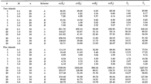
TABLE 3

Variances of four estimators under the neutral Wright’ f~te-islands model

Two islands 5 5

0.1 5

1

.o

5.0 5

5

0.1 1.0

5 5.0

20 0.1

20 1

.o

20 5.0 20 0.1

20 1.0

20 5.0

Five islands

5 0.1

5 5 1.0 5.0 5 5 0.1 1.0 5 5.0

20 0.1

20 1.0

20 5.0

20 0.1

20 1.0

20 5.0

20 20 20 20 20 20 50 50 50 50 50 50 20 20 20 20 20 20 50 50 50 50 50 50 A A A B B B A A A B B B A A A B B B A A A B B B 49.05 10.53 7.28 15.35 7.32 7.09 851.70 144.27 101.82 236.94 100.03 95.71 114.19 16.49 8.09 8.50 6.79 6.18 1709.09 253.37 117.48 133.40 99.82 92.79 29.03 6.25 4.28 10.52 4.09 3.88 439.10 62.67 41.91 133.96 39.68 34.80 68.84 11.03 4.98 6.54 3.75 3.27 1052.06 126.98 55.45 95.90 41.75 33.54 6.50 4.54 3.37 2.66 2.62 2.52 36.69 31.14 22.45 15.80 15.73 15.63 32.99 9.46 3.66 3.29 1.95 1.94 360.56 86.01 31.35 30.76 14.91 13.79 28.58 6.00 4.14 8.39 3.89 3.67 432.95 59.14 37.35 69.53 30.92 26.87 68.86 11

.oo

4.92 5.80 3.39 3.00 1085.31 124.31 53.59 86.94 31.65 25.45 7.21 5.60 4.43 2.68 3.24 3.71 37.52 38.18 29.81 16.11 18.37 20.53 36.95 12.23 5.14 4.72 2.87 2.84 373.79 111.24 44.27 40.33 18.91 17.87 29.88 8.17 6.30 8.22 5.04 5.32 442.44 80.55 56.50 81.32 42.98 42.25 73.34 17.25 8.16 10.36 6.06 5.20 1227.03 205.75 90.85 127.38 55.11 42.23 Note; a and 8 are estimated from 10,000 samples and the results in each row of the table is from 10,000 samples. A, extreme sampling scheme;

B, balanced sampling scheme. Also see the footnote to Table 1 for sv, V E and

vq.

that all the islands have the same effective population size Nand that the overall migration rate m is sufficiently small so that the probability that two or more individuals in a sample migrate at the same generation can be neglected. Also we assume that there is no recombination. An event under the WRIGHT’S finite-islands model is either a coalescence or a migration. A coalescence event reduces by one the number of ancestral genes in the island where the coalescence event occurs while a migration event reduces by one the number of ancestral genes in one island but increases by one the number of ancestral genes in another island, thus the total number of ancestral genes remains the same. Let M = 4Nm and 6, ( k = 1,

. . .

,

d ) be the number of ancestral genes in island k between two consecutive events. STROBECK (1987) showed that the expected time length between the two events is

4N

bk

+

x h6k(6h - l) ’

Algorithms for generating samples under the neutral Wright’s finite-islands model were developed by STROBECK (1987) and SLATKIN and MADDISON (1989).

Since there is no recombination, all the sites in the sequences have the same genealogy. However, unlike the model with recombination, the expectation of the number of i-mutations is no longer the same as that un-

der the neutral Wright-Fisher model. Therefore, &,is no longer the same as K , neither is

6,

as

.ir.

Because migrations tends to increase the time between two coalescent events,

K

and

7i

both overestimate 8.

We focus on the cases of two islands and five islands and consider two sampling schemes. The first is that all the sequences are taken from one island and the second is that a sample is taken from each island. These two sampling schemes will be referred to as the extreme- sampling scheme and the balanced-sampling scheme respectively and consequently a sample from the extreme- sampling scheme and a sample from the balanced sampling scheme will be will be referred to as an extreme sample and a balanced sample, respectively.

We again use simulated samples to evaluate the performances of the four estimators. Table 3 summarizes the results of simulations. It is obviously that

d,

is again the best estimator among the four estimators, but all of them have smaller variances when migration rate is large than when migration rate is small. Similar to the neutral WRIGHT-FISHER model and the neutral model with recombination, superiority of

d,

is mostly evident when 8 and sample size TZ are both large and in such cases,

d,

also shows considerable improvement over

dK dT

is again the worst estimator among the four.

(10)

el

L"

r

0 1 2 3 4 5

A i

/

-

I

0 1 2 3 4 5

M

FIGURE 5.-Coefficients of

de

(panel a) and

e,,

(panel b) as

functions of migration parameter M for balanced samples of size 10 from two islands. The curves from top down represent y,

. . .

, in panel a and v,,

. . .

, v, in panel b. The coefficients

for each value of M are averaged over 10,000 samples and

0 = 20.

scheme, all the estimators performs better in the case of two islands than in the case of five islands, suggesting that in general the variance of an estimator of 8 increases with the number of islands under the extreme-sampling scheme. For the balanced-sampling scheme, the pat- terns of the four estimators are not all the same. When Mis small,

6,

and

6,

perform better with smaller number of islands than with larger number of islands but the re- verse are true when M is relatively large. In comparison,

6,

and

6,

seem to perform better with larger number of islands for all the migration rates we have considered. Table 3 also shows that the balanced-sampling scheme is always better than the extreme-sampling scheme for the purpose of estimating 8 because all the estimators perform better under the former scheme than under the latter one. The extreme sampling scheme should be avoided particularly when migration rate is small. It should be pointed out that we have assumed that all islands have the same effective population size in our

TABLE 4

Variances of four estimators under the infinite-loci neutral model

with recombination when R has to be estimated

e

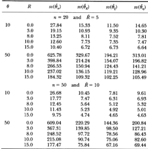
R s 4 e , ) 4 4 i ) su(@*) 4 l )

10 50 10 50 0.0 3.0 8.0 10.0 15.0 0.0 3.0 8.0 10.0 15.0 0.0 3.0 8.0 10.0 15.0 0.0 3.0 8.0 10.0 15.0

n = 2 0 and k = 5

27.84 15.33

19.15 10.93

13.25 8.11

12.60 7.73

10.40 6.72

625.78 329.67

398.84 214.24

266.53 150.94

237.02 136.15

184.32 109.32

n = 50 and k = 10

26.68 10.45

17.77 7.47

12.45 5.64

11.43 5.23

9.75 4.74

609.04 220.29

367.31 139.85

248.52 97.72

215.08 90.74

177.47 75.84

11.50 9.35 7.52 7.35 6.73 194.21 154.07 124.43 119.21 102.25 7.81 6.31 5.12 4.92 4.65 144.36 98.50 78.56 75.06 67.16 14.65 10.30 7.81 7.47 6.64 313.01 196.82 141.21 128.96 105.49 9.61 6.93 5.32 5.01 4.63 200.84 127.21 86.43 82.60 69.44

Estimations of a and I; are based on estimated k and 10,000 samples. Each row is obtained from 10,000 simulated samples with recombination rate R. Also see the footnote to Table 1 for su,

vt

and

vq.

simulations. When this is not true, the best sampling scheme is likely the generalized balanced-sampling scheme in which the relative size of a sample from an island with respect to the overall sample size is the same as the relative value of the effective population size of the island with respect to the sum of all effective population sizes.

We also present in Table 3 the means of estimated variances of

6,

and

6,.

It is found that variances of and

6,

computed from Equations 19 and 20, respectively are on average overestimates of the true variances under the neutral Wright's finite-islands model.

The coefficients of

6,

and

6,

for a balanced sample of size 10 from two islands are given in Figure 5. It is in- teresting to see that the coefficients quickly become stable with the value of M. This example and many oth- ers we examined indicate that as far as 8 is concerned, samples from islands may be treated as from a panmictic population even when migration parameter Mis as small as 1, particularly when the estimator

6,

is used. This o b servation is in accordance with a large body of literature showing that migration is extremely powerful in elimi- nating differences among local populations. Under the neutral Wright's finite-islands model, the coefficients of

6,

and

6,

also satisfy the relationship given by (27) which seems to be true in general.

DISCUSSION

(11)

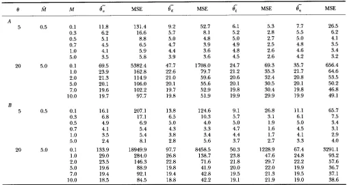
TABLE 5

Means and MSE of the four estimators under the neutral Wright’s finiteislands model for balanced samples

0 M M

0 -

,

MSE MSE 9 s MSE

e;

MSE

-

6,

-

A

5 0.5 0.1 11.8 131.4 9.2 52.7 6.1 5.3 7.7 26.5

0.3 6.2 16.6 5.7 8.1 5.2 2.8 5.5 6.2

0.5 5.1 8.8 5.0 4.8 5.0 2.7 5.0 4.1

0.7 4.5 6.5 4.7 3.9 4.9 2.5 4.8 3.5

1

.o

4.1 5.9 4.4 3.6 4.8 2.6 4.6 3.4

5.0 3.5 5.8 3.9 3.6 4.5 2.6 4.2 3.2

20 5.0 0.1 69.5 5382.4 47.7 1708.0 24.7 69.3 35.7 656.4

1.0 23.9 162.8 22.6 79.7 21.2 35.3 21.7 64.6

2.0 21.3 114.9 21.0 59.6 20.6 32.4 20.8 53.5

5.0 20.1 106.0 20.1 55.6 20.1 30.5 20.1 50.2

7.0 19.6 102.2 19.7 52.9 19.8 30.4 19.8 46.8

10.0 19.7 97.7 19.8 51.9 19.9 29.9 19.9 49.1

5 0.5 0.1 16.1 207.1 13.8 124.6 9.1 26.8 11.1 65.7

0.3 6.8 17.1 6.5 10.3 5.7 3.1 6.1 7.5

0.5 4.9 6.9 5.0 4.0 5.0 1.9 5.0 3.4

0.7 4.1 5.4 4.3 3.3 4.7 1.6 4.5 3.1

1

.o

3.5 5.4 3.8 3.4 4.4 1.7 4.1 2.9

5.0 2.4 8.1 2.8 5.6 3.7 2.7 3.3 4.0

20 5.0 0.1 133.9 18949.9 97.7 8458.5 50.3 1228.9 67.4 3291.1

1

.o

29.0 284.0 26.8 138.7 23.8 47.6 24.8 93.2

2.0 23.5 146.3 22.8 71.6 21.8 29.7 22.2 57.6 5.0 19.6 88.9 19.8 41.9 20.0 22.0 19.9 36.7

7.0 19.4 92.1 19.4 42.8 19.5 21.3 19.5 37.1

10.0 18.5 84.5 18.8 42.2 19.1 21.9 19.0 38.6

B

- ”

e,, e,,

6, and

e,

are, respectively, the means of

e,, e,, e,

and

e,.

Estimations of a and 2 are based on estimated value M of M and 10,000 samples. Each row is obtained from 10,000 samples. A, Two islands and 10 sequences are taken from each island; B, five islands and five sequences

-

are $ken from each island.

and the neutral Wright’s finite-islands model that the

6,

is an efficient estimator of 8. However, comparisons of the performances of various estimators were conducted assuming that the values of parameters other than 8 are known. Since in practice the value of migration parameter M and the value of recombination parameter R are likely unknown as well, one has to estimate their values in order to obtain estimates of 8 by

GC

or

0,.

It then raises a question: will

0,

be still superior when M and R are to be estimated? Although the recombination parameter R can be estimated by, for example, HUDSON and KAPLAN’S (1987) method or HUDSON’S (1993) method and the migration parameter M by, for example, SLATKIN and

MADDISON’S (1989) method, but their inferences are still

in their infancies and better methods for estimating M and R are likely to appear in the near future. Therefore

I decide to examine the performances of the four estimators by using directly erroneous values of M or R to estimate a and

2.

Consider the neutral model with recombination first. Since recombinations do not change the expectation of

5

and r), it is easy to see that

6,

and

6,

is still unbiased estimators of 8, when the estimated value of R is inac- curate. Table 4 gives a few examples on how the variances of

6,

and

6,

are affected when the estimate of R is inaccurate. It is found from Table 4 that

6,

remains to be the best estimator even when the estimate R of R is considerably different from its true value. However, when R is different from R, the variances of

6,

and

0,

increase. For example, consider the case of 8 = 50 and sample size n = 50, when R is equal to 0 while it is estimated to be 10, the variances of

6,

and

6,

are, respectively, 144.4 and 200.8 (Table 4), but if the estimation of R is accurate, i . e . , R = 0, the variances become 92.3 and 166.9 respectively (Table 1). These simulations show that the effort to compute

0,

is undoubtedly worthwhile and one must make effort to obtain good estimate of R to make most of

6,.

Next we consider the neutral Wright’s finite-islands model. When the estimate Mof Mis not accurate, all the four estimators become biased. To measure the per- formance of a biased estimator we must consider its bias as well as its variance. A proper measure of the accuracy of a biased estimator

6

of 8 is the mean square error (MSE)

,

defined by

MSE =

E(6

- = Var(6)

+

(6

-

Note that when

6

is unbiased, MSE is simply the variance of

6.

Since the balanced-sampling scheme is much better than the extreme-sampling scheme and its use is strongly recommended, I shall examine the performances of the four estimators for balanced samples only. Table 5 gives a few examples of the effect on estimations of 8 when M is not accurate.

It is clear from Table 5 that all the four estimators,

(12)

a superior estimator not only because its MSE is the smallest in all the cases we examined but also because it is the least biased estimator. Table 5 also shows that the MSE of each estimator becomes relatively large when M is much larger than M; while on the other hand, the MSE of an estimator does not change substantially when

fi

is considerably smaller than M . This suggests that for the purpose of estimating 8 it is better to underestimate M

than to overestimate M . We pointed out earlier by examining the coefficients of

6,

and

6,

that samples from islands may well be treated as from a panmictic population when M is not extremely small and Table 5 re- inforces this conclusion. For example, when

&

is 5 which may be regarded to represent a nearly panmictic population, the bias of is not substantial when M is as small as 1, through the bias seems to increase with the number of islands.

We assumed in this paper that the frequencies of mutations of various sizes, i. e.

6,

can be inferred accurately, which implies that either the infinite-sites model is ap- propriate and an outgroup sequence is available, or the sequences are sufficiently long so that the phylogeny reconstruction is accurate. Samples of sequences of modest length without an outgroup are common and thus procedure for estimating 8 for such samples will be of practical importance. Because Lj and r) are also likely to be important in constructing more powerful tests of the hypothesis of neutral mutations than those by TAJIMA (1989) and Fu and LI (1993b), and may even lead to better estimators of R and M , we are currently searching for the best methods to infer the values of

6

and r) under

various population models. But without going further, we expect that when the values of Lj and r) can not be inferred accurately, some simple equations for bias cor- rection may be sufficient in practice, as found for a BLUE of 8 by Fu (1994a). For the neutral Wright’s finite- islands model, it may turn out that the bias due to estimating M is larger than that due to estimating

6

and r) therefore finding a good estimate of M may be more critical.

The programs written in C language for estimating 8 under models considered in this paper are available from the author whose E-mail address is [email protected].

I thank an anonymous referee for suggestions. This work is s u p

ported in part by a FIRST AWARD from the National Institutes of Health.

LITERATURE CITED

FELSENSTEIN, J., 1992 Estimating effective population size from samples of sequences: a bootstrap monte carlo integration method. Gen. Res. 60: 209-220.

Fu, Y. X., 1994a A phylogenetic estimator of effective population size or mutation rate. Genetics 136: 685-692.

Fu, Y. X., 1994b Statistical properties of segregating sites. Theor. Popul. Biol. (in press).

Fu, Y. X., and W. H. LI, 1993a Maximum likelihood estimation of

population parameters. Genetics 134: 1261-1270.

Fu, Y. X., and W. H. LI, 1993b Statistical tests of neutrality of mutations. Genetics 133 693-709.

HAMMERSLEY, J. M., and D. C. HANDSCOMB, 1965 Monte-Curlo Meth- ods. John Wiley & Sons, New York.

HUDSON, R. R., 1983 Properties of a neutral allele model with intra- genic recombination. Theor. Popul. Biol. 23: 183-201.

HUDSON, R R, 1993 The how and why of generating gene genealogies, pp 23-38 in Mechanisms ofMoIemlarEvolutia, edited by N. TAKAHATA and A. G. CWUL Sinaur Associates, Sunderland, Mass.

HUDSON, R. R., and N. L. KAPLAN, 1985 Statistical properties of the number of recombination events in the history of a sample of DNA sequences. Genetics 111: 147-164.

KINGMAN, J. F. C., 1982a The coalescent. Stochast. Proc. Their Appl.

13: 235-248.

KINGMAN, J. F. C., 1982b On the genealogy of large populations. J. Appl. Prob. 19A: 27-43.

SLATKIN, M., and W. P. MADDISON, 1989 A cladistic measure of gene

flow inferred from the phylogenies of alleles. Genetics 123:

603-613.

STROBECK, C., 1987 Average number of nucleotide difference in a sample from a single subpopulation: a test for population sub-

division. Genetics 117: 149-153.

TAJIMA, F., 1983 Evolutionary relationship of DNAsequences in finite populations. Genetics 105: 437-460.

TAJIMA, F., 1989 DNA polymorphism in a subdivided population: the expected number of segregating sites in the mesubpopulations model. Genetics 123: 229-240.

WATTERSON, G . A,, 1975 On the number of segregation sites. Theor. Popul. Biol. 7: 256-276.