Nonlinear Transportation Problems Algorithm

Nonlinear Transportation Problems’ Algorithm

(A Case Study of the Nigerian Bottling Company Ltd Owerri Plant)

Opara Jude1_{, Iheagwara Andrew .I.}2 _{& Nwobi Anderson Chukwukailo}3

1_{E-mail Address: [email protected]}

Department of Statistics, Imo State University PMB 2000, Owerri Nigeria

GSM: +2348064095411

2_{E-mail Address: [email protected]}

Procurement Officer/Director Planning, Research & Statistics, Nigeria Erosion & Watershed Management Project (World Bank-Assisted), Ministry of Petroleum & Environment, Ploy 36, chief Executive Quarters, Area “B”, New Owerri, Imo State

Nigeria GSM: +2348033285954

3_{E-mail Address: [email protected]}

Department of Statistics, Abia State Polytechnic, Aba Nigeria GSM: +2348036018752

ABSTRACT

This study is centered on the nonlinear Transportation problems Algorithms using Nigerian Bottling Company Ltd Owerri Plant as a case study. This paper is intended to determine the quantity of Fanta, Coca-Cola, Schweppes and Sprite (all in crates) that the Company should distribute in a month in order to minimize the cost of transportation and maximize profit. A problem of this nature was identified as a Nonlinear

Transportation Problem (NTP),

formulated in mathematical models and

tackled by the Karush-Kuhn-Tucker

(KKT) optimality condition for the NTP.

A statistical software package was used to obtain the initial basic feasible solution using the Least Cost Method. Thus, the result of the analysis revealed

that the optimal solution that gave minimum achievable cost of supply was the supply of 8000 crates of Sprite and 5000 crates of the same product to

Umuahia market zone and Eket

respectively; 12000 crates of Coca-cola, and 4000 crates of the same product to Nnewi and Eket respectively; 9000 crates and 2000 crates of Schweppes product to Aba, and Umuahia market zones respectively; 1000 and 14000 crates of Fanta to Aba and Orlu market zones respectively., at a total cost of N509, 000.

Key words:

Karush-Kuhn-Tucker_,

1. Introduction

In the linear transportation problem (ordinary transportation problem) the cost per unit commodity shipped from a given source to a given destination is constant, regardless of the amount shipped. It is always supposed that the mileage (distance) from every source to every destination is fixed. To solve such transportation problem we have the streamlined simplex algorithm which is very efficient. However, in reality, we can see at least two cases that the transportation problem fails to be linear.

First, the cost per unit commodity transported may not be fixed for volume discounts sometimes are available for large shipments. This would make the cost function either piecewise linear or just separable concave function. In this case the problem may be formulated as piecewise linear or concave programming problem with linear constraints.

Second, in special conditions such as transporting emergency materials when natural calamity occurs or transporting military during war time, where carrying network may be destroyed, mileage from some sources to some destination are no longer definite. So the choice of different measures of distance leads to nonlinear (quadratic, convex, etc.) objective function.

In nonlinear transportation problem, its solution is more complex than that of linear transportation problem. In this work, solution procedures to the generalized transportation problem taking nonlinear cost function are

investigated. In particular, the nonlinear transportation problem considered in this paper is stated as follows;

• We are given a set of n sources of commodity with known supply capacity and a set of m destinations with known demands.

• The function of transportation cost is nonlinear and differentiable for a unit of product from each source to each destination.

• We are required to find the amount of product to be supplied from each source (may be market) to meet the demand of each destination in such a way as to minimize the total transportation cost.

Our approach to solve this problem is applying the existing general nonlinear programming algorithms to it making a suitable modification in order to use the special structure of the problem.

focus will be to develop a mathematical model using optimization techniques to close the demand and supply gap by discounting so as to minimize total transportation cost. This research seeks to apply the existing general nonlinear programming algorithms to solve our problem

2. Review of related Literatures

Zangiabadi and Maleki (2007) presented a fuzzy goal programming approach to determine an optimal compromise solution for the multi-objective transportation problem by assuming that each objective function has a fuzzy goal. A special type of non-linear (hyperbolic) membership function is assigned to each objective function to describe each fuzzy goal. The approach focused on minimizing the negative deviation variables formed to obtain a compromise solution of the multi-objective transportation problem.

Ekezie and Opara (2013) carried out a research on the transportation algorithm with volume discount on distribution cost using Port Harcourt flour mills company Ltd as a case study. The research was intended to determine the quantity of Golden Penny Flour (in 50kg bags), Golden Penny Semovita (in 10kg bags) and Wheat Offals (also in 50kg bags) that Port Harcourt Flour Mills Company should distribute in a month in order to minimize transportation cost and maximize profit. A problem of this nature was identified as a Nonlinear Transportation Problem (NTP), formulated in mathematical terms and solved by the KKT optimality condition for the NTP. The initial basic feasible

solution using Vogel Approximation Method (VAM) was obtained. The result of the analysis revealed that optimality occurred at the second iteration and allocations were made.

Lau et al. (2009) presented an algorithm called the fuzzy logic guided non-dominated sorting genetic algorithm to solve the multi-objective transportation problem that deals with the optimization of vehicle routing in which multiple depots, multiple customers, and multiple products were considered. Since the total traveling time is not always restrictive as a time constraint, the objective considered comprises not only the total traveling distance, but also the total traveling time. Lohgaonkar and Bajaj (2010) used fuzzy programming technique with linear and non-linear membership function (hyperbolic, exponential) to find the optimal compromise solution of a multi-objective capacitated transportation problem.

Ekezie et al (2013) carried out a research on the determination of paradoxical pairs in a linear transportation problem. In their study, an efficient algorithm for solving a linear programming problem was discussed, and it was concluded that paradox exists. The North-West Corner method was used to obtain the initial basic feasible solution for the optimal solution. They also used the algorithm discussed to develop a step by step solution procedure for finding all the paradoxical pairs.

aggregation of customer orders in separate full-truckload or less-than-truckload shipment in order to minimize total transportation cost. He has demonstrated that evolutionary computation technique may be effective in tactical planning of transportation activities. The model shows that substantial savings on overall transportation cost may be achieved by adopting the methodology in a real life scenario.

Kikuchi (2000): Suggested that in many problems of transportation engineering and planning, the observed or derived values of the variables are approximate, yet the variables themselves must satisfy a set of rigid relationships dictated by physical principle. They proposed a simple adjustment method that finds the most appropriate set of crisp numbers. The method assumes that each observed value is an approximate number (or a fuzzy number) and the true value is found in the support of the membership

function. This process was performed using the fuzzy linear programming method for each of many possible sets of values for the problem.

Ekezie et al (2013) in their research on paradox, a transportation problem with an objective function as the sum of a linear and linear fractional function was considered. The result of their analysis showed that a paradoxical situation arises in the sum of a linear and linear fractional transportation problem, when value of the objective function falls below the optimal value and this lower value was attainable by transporting larger number of passengers. An algorithm was discussed for finding initial basic feasible solution for the sum of a linear and linear fraction transportation problem and a sufficient condition for the existence of a paradoxical solution was established. Data collected from a secondary source were used for the explanation of the algorithm.

3. Methodology

3.1 THE KARUSH-KUHN-TUCKER (KKT) OPTIMALITY CONDITION

FOR NONLINEAR PROGRAMMING PROBLEM

Given the non linear programming problem (NNP): min f(x)

s.t. gi(x) ≤ 0 i = 1, …, k … (1)

hj(x) = 0 j = 1, …, l

3.1.1 KARUSH-KUHN-TUCKER NECESSARY OPTIMALITY

CONDITIONS

Theorem 1: Given the objective function f :_ℝn → _{ℝ and the constraint function are g} i

:_ℝn → _{ℝ and h}

j : ℝn → ℝ and I = {i: gi(x*) = 0}. In addition, suppose they are

1, …, l be linearly independent. If x* is minimizer of the problem (NPP), then there exist scalars λ_i; i = 1, …, k and µj; j =1, …, l, called Lagrange multipliers, such that

∑

∑

= =

= ∇ µ + ∇

λ +

∇ k

1

i j1

j j i

i g (x*) h x* 0 *)

x ( f

l

0 *) x ( g_i i =

λ … (2)

0 i≥

λ ; µj∈ℝ

3.1.2 KARUSH-KUHN-TUCKER SUFFICIENT OPTIMALITY

CONDITIONS FOR CONVEX NPP

Further, if f and each gi are convex, each hj is affine, then the above necessary optimality

conditions will be also sufficient (Simons; 2006).

Justification

Let x be any feasible point different form x*. From the first KKT conditions we obtain

    

  

− ∇

µ + − ∇

λ − = −

∇

∑

∑

= =

k

1

i j1

j j t

i

i g (x*)(x x*) h (x*)(x x*) *)

x x *)( x ( f

l

Since each gi(x) is convex, λi ≥0 and ∇hj(x*)(x – x*) = 0 ∀j, we also have

] *) x ( g ) x ( g [ *)

x x *)( x ( g k

1 i

k

1 i

i i

i t

i i

∑

∑

= =

− λ

≤ − ∇

λ

⇒ _∇f(x*)(x₋x*)_≥−

∑

_λig_i(x)_≥0

From convexity of f(x), therefore, we get f(x) – f(x*) ≥ 0

⇔ f(x*) ≤ f(x) for any feasible x.

4. SOLUTION PROCEDURES TO THE NONLINEAR TRANSPORTATION

PROBLEM (NTP)

In this section, we consider a transportation problem with nonlinear cost function. We try to find different solution procedures depending on the nature of the objective function. Before going to the different special cases, let’s formulate the KKT condition and general algorithm for the problem.

Given a differentiable function C : ℝnm → _ℝ.

We consider a nonlinear transportation problem (NTP) min C(x)

s.t. Ax ≤ _{b … (3)}

                = nm ij 11 x x x x M M ;                     = m 1 n 1 d d s s b M M ;                                 = 1 1 1 1 1 1 1 1 1 1 1 1 1 1 1 1 1 1 1 1 1 1 1 1 1 1 1 1 1 1 A O M M M K M M M K

The KKT Optimality Condition for the NTP The transportation table is given as:

11 x ) x ( C ∂ ∂ … … … m 1 x ) x ( C ∂

∂ s1 _u1

… … … … … … ij x ) x ( C ∂

∂ … … si

i u 1 n x ) x ( C ∂ ∂ … … … nm x ) x ( C ∂

∂ sn un

d1 … dj … dm

1

v … vj … vm

where x is the current basic solution.

The Lagrange function for the NTP is formulated as

z(x, λ, w) = C(x) + w(b – Ax) – λx … (4) where λ and w are Lagrange multipliers and

The optimal point x should satisfy the KKT conditions: ∇z = ∇C( x ) – wT_{A –} λ _{= 0}

λx = 0 λ ≥ 0

x ≥ 0

Specifically for each cell (i, j) we have

0 )

e , e )( v , u ( x

) x ( C x

z

ij j n i ij

ij

= λ − −

∂ ∂ = ∂

∂

+ … (5)

λijxij = 0

xij ≥ 0

λij ≥ 0

Where k = 1 … nm and w = (u, v) = (u1 u2… un, v1… vm), ek∈ℝm+n is a vector of zeros

except at position k which is 1.

From the conditions (5) and λk ≥ 0, we get,

0 ) v u ( x

) x ( C x

z

j i ij ij

≥ + − ∂ ∂ = ∂

∂

… (6)

0 ) v u ( x

) x ( C x x

z

x i j

ij ij ij

ij =

  

  

+ − ∂ ∂ = ∂

∂

… (7)

xij ≥ 0

General solution procedure for the NTP • Initialization

Find an initial basic feasible solution x • Iteration

Step I: if x is KKT point, stop. Otherwise go to the next step.

Step II: Find the new feasible solution that improves the cost function and go to step

1(Kidist; 2007)

5. TRANSPORTATION

PROBLEM WITH CONCAVE COST FUNCTIONS

For large distributions, volume discount may be available sometimes. In this case the cost function of the transportation problem generally takes concave structure for it is separable and the marginal cost (cost per unit commodity distributed) decreases with increase in the amount of distribution; because of the total cost increase per addition of

unit commodity distributed. The discount

1. May be either directly related to the unit commodity.

2. Or have the same rate for some amount.

Case 1: If the discount is directly related

min C_ij(x_ij) m

1 j n

1 i

∑

∑

= =

i ij m

1 j

s x t .

s

∑

= =

j = 1, 2, …, m … (8)

j ij n

1 i

d x =

∑

=

i = 1, 2, …, n;

Where Cij : ℝ→ℝ

6. THE TRANSPORTATION CONCAVE SIMPLEX ALGORITHM (TCS)

Initialization

Find the initial basic feasible solution using some rule like west corner rule.

Iteration

Step 1: Determine the values of ui and vi from the equation,

0 ) v u ( x

) x ( C

j i Bij

= + − ∂ ∂

… (9)

Where xBij are the basic variables.

Step 2: If

0 ) v u ( x

) x ( C

j i ij

≥ + − ∂ ∂

… (10)

for all xij – non basic, stop, x is KKT point. Otherwise go to step 3.

Step 3: Calculate

    

  

− − ∂ ∂ = ∂

∂

j i ij r

v u x

) x ( C x

z

l

… (11)

xrl will enter the basis. Allocate xrl = θ

where θ is found as in the linear transportation case.

Adjust the allocations so that the constraints are satisfied.

Determine the leaving variable say xBrk,

where xBrk is the basic variable which

comes to zero first while making the adjustment. Then find the new basic variables and go to step 1.

7. Data Analysis

The Nigerian Bottling Company Ltd (NBC) operates 13 plants in Nigeria, which Owerri is one of the plants. NBC

operates Owerri Plant since 1982 and is located in the capital city of Owerri in Imo State in South-East Nigeria. The Owerri Plant is responsible for the production of Coca-Cola, Fanta, Sprite and Schweppes and distribution of all product categories.

.

Table 1: Cost of Transporting the Drinks to the various market zones.

Products Availability Market segments

Aba Umuahi a

Nnewi Orlu Eket Supply

Sprite 13000 13 9 10 11 9 13000 Coca-Cola 16000 12 10 7 14 9 16000 Schweppes 11000 14 11 15 12 15 11000 Fanta 15000 12 16 13 8 14 15000 Requirement of Drinks 10000 10000 12000 14000 9000 55000

All the value in the Table 1 apart from requirements and supply are in Nigerian Currency (Naira) value. The Policy of the Company assumes discounts on each product transported from source to destination and it is directly related to the unit commodity purchased and transported, and the percentage discounts are shown in Table 2.

Table 2: Percentage Discounts

Aba Umuahia Nnewi Orlu Eket

Sprite 0.02 0.03 0.02 0.02 0.005

Coca-Cola 0.03 0.01 0.02 0.013 0.015 Schweppes 0.02 0.04 0.04 0.02 0.05

Fanta 0.014 0.02 0.03 0.05 0.01

The problem is to determine how many creates of each product to be transported from the source to each destination on a monthly basis in order to minimize the total transportation cost.

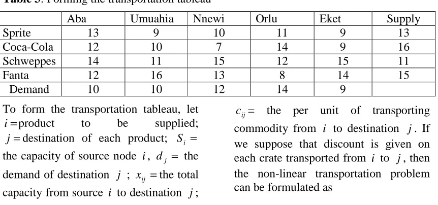
Table 3: Forming the transportation tableau

Aba Umuahia Nnewi Orlu Eket Supply

Sprite 13 9 10 11 9 13

Coca-Cola 12 10 7 14 9 16

Schweppes 14 11 15 12 15 11

Fanta 12 16 13 8 14 15

Demand 10 10 12 14 9

To form the transportation tableau, let =

i product to be supplied; =

j destination of each product; Si =

the capacity of source node i , d_j = the

demand of destination j ; xij =the total

capacity from source i to destination j ;

ij

c = the per unit of transporting

Minimize

+ + + + + + + + + + + + +

+ 12 13 14 15 21 22 23 24 25 31 32 33 34

11 9 10 11 9 12 10 7 14 9 14 11 15 12

13x x x x x x x x x x x x x x

45 44

43 42

41

35 12 16 13 8 14 15x + x + x + x + x + x

Subject to:

x₁₁+x₁₂ +x₁₃ +x₁₄ +x₁₅ =13000

x21+x22 +x23+x24 +x25 =16000 x31+x32 +x33+x34 +x35 =11000 x₄₁+x₄₂ +x₄₃+x₄₄ +x₄₅ =15000

x11+x21+x31 +x41 =10000 10000 42

32 22

12 +x +x +x =

x

12000 43

33 23

13 +x +x +x =

x

14000 44

34 24

14 +x +x +x =

x

9000 45

35 25

15 +x +x +x =

x

Where

2 11 11 11 11

11x 13x p x

c = − c31x31 =14x31−p31x312

2 12 12 12 12

12x 9x p x

c = − c32x32 =11x32 −p32x322

2 13 13 13 13

13x 10x p x

c = − 2

33 33 33 33

33x 15x p x

c = −

2 14 14 14 14

14x 11x p x

c = − c₃₄x₃₄ =12x₃₄ − p₃₄x₃₄2

2 15 15 15 15

15x 9x p x

c = − c35x35 =15x35 −p35x352

2 21 21 21 21

21x 12x p x

c = − c41x41 =12x41−p41x412

2 22 22 22 22

22x 10x p x

c = − c₄₂x₄₂ =16x₄₂ −p₄₂x₄₂2

2 23 23 23 23

23x 7x p x

c = − 2

43 43 43 43

43x 13x p x

c = −

2 24 24 24 24

24x 14x p x

c = − c₄₄x₄₄ =18x₄₄ −p₄₄x₄₄2

2 25 25 25 25

25x 9x p x

c = − c₄₅x₄₅ =14x₄₅ −p₄₅x₄₅2

If we allow the following discounts on each transported product I from the source to each of the destinations, we obtain the cost function c which can be expressed as; _ij

2 11 11

11

11x 13x 0.02 x

c = − c31x31 =14x31−0.02x312

2 12 12

12

12x 9x 0.03x

c = − c32x32 =11x32 −0.04x322

2 13 13

13

13x 10x 0.02x

c = − 2

33 33

33

33x 15x 0.04x

c = −

2 14 14

14

14x 11x 0.02x

c = − c₃₄x₃₄ =12x₃₄ −0.02x₃₄2

2 15 15

15

15x 9x 0.005x

c = − c₃₅x₃₅ =15x₃₅ −0.05x₃₅2

2 21 21

21

21x 12x 0.03x

c = − c41x41 =12x41−0.014x412

2 22 22

22

22x 10x 0.01x

2 23 23

23

23x 7x 0.02x

c = − c43x43 =13x43 −0.03x432

2 24 24

24

24x 14x 0.013x

c = − c44x44 =8x44 −0.05x442

2 25 25

25

25x 9x 0.015x

c = − c₄₅x₄₅ =14x₄₅−0.01x₄₅2

The tableau is then developed as below;

Aba Umuahia Nnewi Orlu Eket S1 ui

Sprite 13000 u ₁

Coca-Cola 16000 u ₂

Schweppes 11000 u ₃

Fanta 12 16 13 8 14 15000

dj 10000 10000 12000 14000 9000

vj v ₁ v ₂ v ₃ v ₄ v ₅

Using the Least Cost method, we get the initial basic solution as shown below.

Aba Umuahia Nnewi Orlu Eket s1 ui

Sprite 13 9

8

10 11 9

5

13000 u1

Coca-Cola 12 10 7

12

14 9

4

16000 u2

Schweppes 14

9

11

2

15 12 15 11000 u3

Fanta 12

1

16 13 8

14

14 15000

dj 10000 10000 12000 14000 9000

vj v ₁ v ₂ v ₃ v ₄ v ₅

(

x11,x 12,x13,x14,x 15,x21,x22,x 23,x24,x 25,x 31,x 32,x33,x34,x35,x 41,x42,x43,x 44,x45

)

x= B B B B B B B B

=

(

0,8,0,0,5,0,0,12,0,4,9,2,0,0,0,1,0,0,14,0

)

, in thousand with the total transportation cost of N509,000.

Now, we use the KKT optimality conditions to improve upon our solution. The partial derivatives at x for the cost function are given as;

13 9 10 11

12 10 7 14 9

14 1 15 12 15

( )

13 11 = ∂ ∂ x x f

( )

8.52 12 = ∂ ∂ x x f

( )

10 13 = ∂ ∂ x x f

( )

11 14 = ∂ ∂ x x f

( )

8.95 15 = ∂ ∂ x x f

( )

₁₂

21 = ∂ ∂ x x f

( )

10 22 = ∂ ∂ x x f

( )

6.52 23 = ∂ ∂ x x f

( )

14 24 = ∂ ∂ x x f

( )

8.88 25 = ∂ ∂ x x f

( )

_13.64

31 = ∂ ∂ x x f

( )

10.84 32 = ∂ ∂ x x f

( )

15 33 = ∂ ∂ x x f

( )

12 34 = ∂ ∂ x x f

( )

15 35 = ∂ ∂ x x f

( )

97 . 11 41 = ∂ ∂ x x f

( )

16 42 = ∂ ∂ x x f

( )

13 43 = ∂ ∂ x x f

( )

6.6 44 = ∂ ∂ x x f

( )

14 45 = ∂ ∂ x x f

Now we find from the cost equation of the occupied cell;

( )

( )

j i Bij j i Bij Bij v u x x f v u x x f x

z _{= +}

∂ ∂ ⇒ = − − ∂ ∂ = ∂ ∂ 0 Thus, 52 . 8 2 1+v =

u u1+v5 =8.95 u2 +v3 =6.52 u2 +v5 =8.88 64

. 13 1 3+v =

u u₃ +v₂ =10.84 u₄ +v₁ =11.97 u₄ +v₄ =6.6

Letting u₁ =0, from the equation above, we obtain; u₁ =0, u₂ =−0.07, ,

32 . 2 3 =

u u₄ =0.65, v₁ =11.32, v₂ =8.52, v₃ =6.59, v₄ =5.95and

95 . 8 5 =

v

We proceed to find the net evaluation factor or the reduced costs for the non-basic variable.

( )

68 . 1 1 1 11 11 = − − ∂ ∂ = ∂ ∂ v u x x f x z

( )

_{3 3} 6.09 33 33 = − − ∂ ∂ = ∂ ∂ v u x x f x z

( )

41 . 3 3 1 13 13 = − − ∂ ∂ = ∂ ∂ v u x x f x z

( )

3 4 3.73 34 34 = − − ∂ ∂ = ∂ ∂ v u x x f x z

( )

_5.05

4 1 14 14 = − − ∂ ∂ = ∂ ∂ v u x x f x z

( )

_{3 5} 3.73 35 35 = − − ∂ ∂ = ∂ ∂ v u x x f x z

( )

75 . 0 1 2 21 21 = − − ∂ ∂ = ∂ ∂ v u x x f x z

( )

4 2 6.83 42 42 = − − ∂ ∂ = ∂ ∂ v u x x f x z

( )

55 . 1 2 2 22 22 = − − ∂ ∂ = ∂ ∂ v u x x f x

z

( )

76 . 5 3 4 43 43 = − − ∂ ∂ = ∂ ∂ v u x x f x z

( )

_1.88

4 2 24 24 − = − − ∂ ∂ = ∂ ∂ v u x x f x

z

( )

Since all the reduced costs for the non-basic variables are all positive, it implies is the KKT optimality point. Because optimal solution is our primary goal, we then proceed to make our allocation.

Hence, the feasible solution that 8000 crates of Sprite and 5000 crates of the same product should be supplied to Umuahia market zone and Eket respectively. 12000 crates of Coca-Cola and 4000 crates of the same product to Nnewi and Eket respectively. 9000 crates and 2000 crates of schwepes product should be supplied to Aba, and Umuahia market zones respectively. 1000, and 14000 crates of Fanta should be allocated to Aba and Orlu market zones respectively. Total cost = 8000 (9) + 5000(9) + 12000(7) + 4000(9) +9000(14) + 2000 (11) + 1000(12) +14000(8)= N509, 000.

8. Conclusion

We have described the transportation problem of Nigerian Bottling Company Ltd Owerri Plant as a non-linear transportation problem. We also applied KKT optimality algorithm to solve the company’s problem. Note that our research centred on the model of the non-linear transportation problem for a particular company in Nigeria. It can however be applied to any situation that can be modeled as such.

This paper aimed at solving transportation problem with volume discount on quantity of goods shipped which is a non-linear transportation problem. Using KKT optimality algorithm, with a set of data from a

Nigerian company Ltd Owerri Plant, it was observed that the optimal solution that gave minimum achievable cost of supply was the supply of 8000 crates of Sprite and 5000 crates of the same product to Umuahia market zone and Eket respectively; 12000 crates of Coca-cola, and 4000 crates of the same product to Nnewi and Eket respectively; 9000 and 2000 crates of Schweppes product to Aba, and Umuahia market zones respectively; 1000, and 14000 crates of Fanta should be allocated to Aba and Orlu market zones respectively, at a cost of N509,000.

Using the more scientific transportation problem model for the company’s transportation problem gave a better result. Management may benefit from the proposed approach for their transportation problem purposes. We therefore recommend that the transportation problem model should be adopted by the company for their transportation problem planning.

References

Caputo, A.C. (2006). A genetic approach for freight transportation planning,

Industrial Management and Data Systems, Vol. 106 No. 5.

Ekezie D. D. and Opara J. (2013). The Application of Transportation Algorithm with Volume Discount on Distribution Cost. Journal of Emerging Trends in Engineering and Applied Sciences (JETEAS). Vol. 4 No. 2.

Ekezie, D.D.; Ogbonna, J.C. and Opara, J. (2013): The Determination of Paradoxical Pairs in a Linear

Transportation Problem.

Mathematics and Statistics Studies. Vol.1, No.3, pp.9-19, September 2013

Ekezie D.D., Opara J., and Mbachu H. I. (2013). Paradoxic sum of Linear and a Linear Fractional Transportation Problem. International Journal of Applied Mathematics and Modeling, IJA2M@KINDI

PUBLICATIONS. Vol.1, No.4, 1-17. October, 2013. ISSN: 2336-0054.

Kidist, T.(2007). Nonlinear Transportation Problems. A paper submitted to the department of mathematics of Addis Asaba University.

Kikuchi, S.A. (2000). A method to defuzzify the number: transportation problem application, Fuzzy Sets and Systems, vol. 116. Lau, H.C.W.; Chan, T.M.; Tsui, W.T.;

Chan, F.T.S.; HO, G.T.S and Choy K.L. (2009). A fuzzy guided multi-objective evolutionary algorithm model for solving Transportation problem. Expert System with Applications: An International Journal. Vol. 36.

Lohgaonkar, M.H. and Bajaj, V.H. (2010). Fuzzy approach to solve multi-objective capacitated transportation problem, International Journal of Bioinformatics Research. Vol. 2. Simons, A.R. (2006). Nonlinear

Programming for Operation research, Society for Industrial and

Applied Mathematics, Vol.10, No.1.

Zangiabadi, M. and Maleki, H.R. (2007). Fuzzy goal programming for

multi-objective transportation

problems. Applied Mathematics