The Relationship among Real Exchange Rate, Current Account Balance and Real Income in Kenya

THE RELATIONSHIP AMONG REAL EXCHANGE RATE, CURRENT ACCOUNT BALANCEAND REAL INCOME IN KENYA

BONIFACE MURIITHI WANJAU

A RESEARCH PROJECT SUBMITTED TO THE DEPARTMENT OF

APPLIED ECONOMICS IN PARTIAL FULFILMENT OF THE

REQUIREMENTS FOR THE AWARD OF MASTER OF ECONOMICS

DEGREE OF KENYATTA UNIVERSITY

DEDICATION

ACKNOWLEGEMENT

I would like to thank the Almighty God for the guidance, protection and direction throughout the study period. Special thanks to my supervisor, Dr. Julius Korir, for his invaluable input and guidance in the study.

TABLE OF CONTENT

TITlE PAGE i

DECLARATION ii

DEDICATION .iii

ACKNOWlEGEMENT iii

TABlE OF CONTENT v

LIST OF FIGURES viii

LIST OF TABLES ix

ABBREVIATIONS AND ACRONYMS x

OPERATIONAL DEFINITION OF TERMS xi

ABSTRACT xi

CHAPTER ONE : 1

1.1. Background of the study 1

1.2. Exchange Rate Movement and Current Account Performance in Kenya 3

1.3. Statement of the problem 8

1.4. Research Questions 10

1.5. Objectives 10

1.6. Significance of the study 10

1.7. Organization of the study 11

CHAPTER TWO 12

2.1. Introduction : 12

2.2. Theoretical Review 12

2.2.2. Elasticity Approach: B-R-M condition 13

2.2.3. Marshall-Lerner Condition 15

2.2.4. Balance of Payment Constraint ModeL 17

2.3. Empirical Review 18

2.4. Overview of Literature 22

CHAPTER THREE 24

3.1. Introduction 24

3.2. Research Design 24

3.3. Theoretical framework 24

3.4. Model Specification 26 -,

3.4.1. Model testing Marshal=-Lerner condition 26

3.4.2. Model testing Thirlwall condition 27

3.5. Definition and measurement of variables 28

3.6. Data sources and data analysis 29

3.7. Data analysis and testing procedure 29

CHAPTER FOUR 32

4.1. Introduction 32

4.2. Descriptive Statistics and Stationarity Analysis 32

4.3. Estimated Results 36

4.3.1. 'Effect of Real exchange rate on current account balance 36

4.3.2. Testing Thirlwall Condition 42

CHAPTER FIVE 48

5.1. Summary ~ 48

5.3. Recommendations 49

LIST OF FIGURES

Figure 1.1: Trending Average Annual Exchange Rate between KSHSIUS$ (1963

to 2012) 4

Figure 1.2:Trending Annual Current Account Balance to GDP ratio from 1975 to

2010

5

Figure 4.1: Trending Import and Export as a percentage of GDP from 1980 to

2011 33

Figure 4.2: Trending GDP and Government Expenditure from 1980 to

2011 34

Figure 4.3: Impulse response function of Change III CAB to

LIST OF TABLES

Table 4.l: Stationarity test results 35

Table 4.2: Co Integration Test 36

Table 4.3: Vector Error Correction Model 37

Table 4.4: Model for testing co integration .42

Table 4.5:Wald test. .43

Table 4.6: Estimates for long run import Model.. 44 Table 4.7: Error Correction Model: Import Model. .45

ARDL

BOP

CAB

DF

ECM

GDP

OLS

IMF

KIPPRA

RER

SDR

USA

USD

VAR

VECM

ABBREVIATIONS AND ACRONYMS Autoregressive Distributed lag Model

Balance of Payment

Current Account Balance

Dickey Fuller

Error Correction Model

Gross Domestic Product

Ordinary Least squares

International Monetary Fund

Kenya Institute for Public Policy Research and Analysis

Real Exchange Rate

Special Drawing Rights

United States of America

United States Dollar

Vector Auto regression

OPERATIONAL DEFINITION OF TERMS

Appreciation: It refers to a rise in value of acountry's currency relative to that of other currencies.

Depreciation: It is a rise reduction in value of a country's currency relative to that of other currencies.

Degree of Openness: It's a tenn used to capture the level of free trade in an economy It refers to the degree to which an economy trades with other economies.

Exchange rate: The value of foreign country's currency in terms of the home country's currency.

Marshal-Lerner-Condition: The Marshall-Lerner condition states that the sum of the elasticities' of demand for a country's exports and of its demand for imports has to be greater than unity for a devaluation to have a positive effect on a country's Balance of Payment. Trade balance: It refers to the current account balance which entails the

ABSTRACT

Persistent current account deficit is a chronic problem in many developing

countries including Kenya. In an attempt to understand disequilibria dynamics in Kenya, this study sought to investigate the effect of real exchange on current account balance and additionally investigate whether the rate of import growth in Kenya is consistent to balanced economic growth as stipulated in Thirlwalllaw. The study is based on two main theories, the neoclassical elasticity approach and balance of payment constraint model. The former contend that balance of

payment is influenced by the nature of import and export elasticities, while the later theory holds that long run economic growth rate may be achieved if growth .of export is consistent with import growth rate. Informed by aforementioned

theories, two main objectives were investigated: First was to determine the effect of real exchange rate change on current account balance in Kenya. Secondly was to determine the extent to which import growth rate is consistent with balanced economic growth in Kenya. The first objective was tested by regressing the trade balance against real exchange rate, foreign income and relative prices, degree of openness and government expenditure. The significance and signage of real exchange rate coefficient was used to determine whether Marshal-Lerner

CHAPTER ONE INTRODUCTION

1.1.

Background of the study

Current account balance (CAB) is a key component of the balance of payment (BOP) and of vital importance in macroeconomic analysis of an open economy. CAB measures current payments (outflows) and current receipts (inflows) between residents of a country and the rest of the world. IMF manual, as quoted in Kariuki (2009), explains that CAB comprises of factor income, balance of transactions of goods and services and current transfers. CAB is an important economic measure of how well an economy fairs in international economic transaction and a key indicator of the level of national savings, spending behavior and investment.

investment III the aforementioned economies (Kariuki, 2009; Ghosh and Ramakrishnan, 2006).

Generally, large and persistent current account deficit may signal ill-performance and vulnerability of the economy. Persistent CAB deficit is also a key indicator of low national savings and investment, lack of international competitiveness and

structural economic problem such as an undeveloped financial system. Furthermore, trade imbalance means a potential loss of output, increased unemployment and unbalanced economic growth (Nusrate, 2008, Ogwuru, 2008; Ghosh and Ramakrishnan, 2006).

According to Ghosh and Ramakrishnan (2006) CAB deficit may be natural and even beneficial to developing countries. Intertempora1 approach argument holds that capita1- deficient countries with high investment opportunities and low national savings may rely on deficit, inform of foreign debt, to spur faster economic growth. This condition can only apply if net foreign borrowings are channeled to investments with higher returns than the cost of capital. Therefore, despite running large CAB deficit, developing countries maybe inter-temporally solvent provided current deficit (liabilities) will be covered by future revenues (Nusrate, 2008; Ogwuru, 2008).

important and strategic macroeconomic fundamental that plays a key role in ensuring a country remains competitive in international trade. It's considered as a strategic tool of economic regulation that maybe formulated in such a way to influence commercial policies and international trade competitiveness of an economy (Dornbursch 1988; Ndung'u, 2001; Ozturk and Acarvci, 2010).

According to Dornbusch (1988), the effectiveness of currency depreciation as a way of improving current account deficit depends on; first, its ability to redirect demand for exports and imports in the right direction and by the right magnitude may determine whether an open economy benefits from trade with the rest of the world. Bird (2001 as cited in Mudida, et

at

2006).

1.2. Exchange Rate Movement and Current Account Performance in Kenya

and Kipyegon 2008). Figure 1.1 shows the real exchange rate trend from 1993 to

2012 estimated using bilateral trade between United States and Kenya

180 160 140 Vi:120 \I) :;) ~ 100 J: \I) =-=: 80

-

I

/

/

/

-

--"

m '<t LI'I co r-, 00 0'10 M N m '<t LI'I co ••...00 0'10 M N

0'1 0'1 0'1 0'1 0'1 0'1 0'10 0 0 0 0 0 0 0 0 0 M M M 0'1 0'1 0'1 0'1 0'1 0'1 0'10 0 0 0 0 0 0 0 0 0 0 0 0

MMMMMMMNNNNNNNNNNNNN

Figure 1.1: Trending Real Exchange Rate inKSHS/US$(1993 to 2012) Source: World Bank Database

Figure 1.1 shows that the real exchange rate trend has been rising gradually from

1993 to 2012. Evidently, the slope of real exchange rate significantly increased

from 2007 to 2012, this may be attributed to inflationary pressure caused by

excess liquidity in the Kenyan economy during this period. Figure 1.2 shows the

current account performance over the three exchange rate policy regime pursued

5

-CAB/GDP ratu

o

U1 ,.... 0'\ 0'\ 0'\ 0'\ .-t .-t Ci:" c ~

.•..

.•..

Q.

-Figure 1.2: Trending Current Account Balance to GDP ratio from 1975 to 2010

Figure 1.2 shows that over the last 38 years, with exception of surpluses recorded

-15

in 200312004 financial year, Kenya has experienced a large and persistent current

-20

One of the main reasons that may explain persistent CAB deficit is the nature of Source: World Bank data base

account deficit.

exports and imports. The Kenyan economy was largely dependent on agriculture

which provided employment to the largest proportion of the working population,

accounting for two thirds of the economy's GDP and up to 40 percent of the

country's export (Kariuki, 2009). Generally, the biggest percentage of Kenyan

exports includes agricultural products such as tea, coffee and horticulture.

Although agricultural horticultural exports and few manufactured goods are

highly responsive to fluctuations in international prices. On the other hand, the

composition of imports are largely price inelastic goods which include machine

and equipment, medical and pharmaceutical products, petroleum, motor vehicle,

telecommunication equipment among others (Ndung'u 2001; Kariuki,

2009;Mudida et ai, 2012).

CAB surpluses registered in 2004 may be attributed to increased tourism and

private current transfers from remittances by Kenyan residents abroad. However,

'despite increase of trade volume, the import ratio has been accelerating factor

than export ratio thus explaining the CAB/GDP trend. The average export to GDP

ratio over the period 1985 to 2006 is 20 percent compared to import to GDP ratio

of 34 percent (Kariuki, 2009).

From independence to 1970's Kenya recorded significant growth owing to rapid

development policy adopted by the government. The GDP growth of over 6.5

percent year-on-year was attributed to increased public investment, pursuance of

import substitution strategy and upsurge of both small scale and large scale

farming. Kenya's reputable performance was attributed to strong macroeconomic

fundamentals including low rates of interest rate, strong exchange rate and a

manageable current account deficit (Kariuki, 2009).

However, the remarkable trend was reversed in the period 1970's to 1980's. A

growing import bill coupled with slowing down of agricultural export earnings

increase in current account deficit. The problem was compounded by the oil crisis in 1973 which led to increase in oil prices by 46 percent. In addition, the collapse of East African community and second oil crisis in 1979 further led to worsening

of the economy's performance during this period (Ndung'u 2001; Kiptui and

Kipyegon 2008, Mudidaet al, 2012).

Prolonged economic problems led to adoption of SAP's in early 1980 are which

included adoption of crawling peg. However, the economy stagnated during the

.period1980 to 1991 due to vulnerabilities, external shocks and lack of proper

implementation. In 1992, significant increase in inflation which was attributed to

general elections of 1992 put pressure on the local currency forcing it to

depreciate (Ndung'u 2001; Kiptui and Kipyegon 2008;Mudida et al, 2012).

Liberalization of interest rate in 1993 led to adoption of floating exchange rate

policy and managed float thereafter. This means that Kenya lost its anchor to major currency thus exposing the domestic economy to direct shocks from

international trade. Evidently, rapid depreciation of Kenya shilling from 1993 to

1999 was accompanied by an unfavorably large current account balance. Large

deficit was attributed to both internal and external shocks such as drought in 1993

and distortion due to speculative tendencies in the foreign exchange market.

However, a break from past trend was witnessed between the years 2003 and

2007. The Kenya shilling appreciated in real terms and the current account

violence and 2011 currency crisis led to a reversal of this trend as the exchange

rate resumed the depreciation trend and worsening of current account balance

(Ndung'u 2001; Kiptui and Kipyegon 2008; Mudida et

at,

Kenya is currently pursuing a managed float policy which requires minimum

intervention by the monetary authority. Liberalization inhibited the use of

exchange rate as a tool for correcting external imbalances and further exposes the

country external shocks and global trade effects. Bird (2001, as cited in Mudidaet

.

at,

vulnerable to speculative attacks as witnessed in Kenyan 2011 exchange rate

crisis where potential gains from depreciation were offset by inflation in the

economy. In this regard, given that significant exchange rate movement are

accompanied by changes in terms of trade as depicted by CAB performance, there

is need to understand the impact of real exchange rate on current account balance

and economic performance under the current policy arena.

1.3. Statement of the problem

Kenya has and continues to experience large and persistent current account

balance deficit over the last three decades. Evidence shows that imports have not

only grown at a faster rate but they are relatively price-inelastic compared to

exports (Kariuki, 2009).

Theoretical and empirical literature identify real exchange rate management as the

(Ozturk and Acaravci, 2009; Ghosh and Ramakrishnan, 2006). However, due to

liberalization, Central Bank of Kenya has lost its control of exchange rate as the

anchor shifted from nominal exchange rate to inflation targeting (Kariuki, 2009;

Mudida et ai, 2012).

Large current account deficit may be beneficial to developing countries if foreign

debt complement low capital formation of the internal economy and consequently

stimulates economic growth (Kariuki, 2009; Ozturk and Acaravci, 2009). On the

other hand, empirical literature shows that running a large and persistent current

account deficit may be risky and even detrimental to the economy (Ghosh and

Ramakrishnan, 2006).

Against this background, increased international trade and global

interdependence, prompts the need to understand the effects of real exchange on

current account balance and economic growth. Kenya, like many other developing

countries, runs a large CAB deficit. To this end, the real debate is the extent to which real exchange rate policies pursued by the economy are sufficient in

eliminating current account deficit and more importantly, promoting

competitiveness of foreign trade III developing countries. This may be

investigated by testing whether real exchange rate targets and policies pursued by

Central Bank of Kenya conform to Marshal-Lerner conditions and Thirlwall

A great part of international macroeconomics literature focuses on issues that

arise when the current account balance is in disequilibrium and its implication on

foreign trade competitiveness. The bulk of empirical studies have focused on

determinants of international trade flows with particular emphasis on the

relationship between current account balance and key macroeconomic variables

(Kariuki, 2009; Tsikata, 2013).The main issue is to evaluate the relationship

among real exchange rates, running a large current account deficit and long run

economic growth. Additionally has the persistent current account deficit been

caused by changes in real exchange rate.

1.4. Research Questions

(i). What is the effect of real exchange rate changes on current account

balance in Kenya?

(ii). Is import growth rate consistent with long run economic growth in Kenya?

1.5. Objectives

(i). To determine the effect of real exchange rate changes on current account

balance in Kenya?

(ii). To determine if import growth rate is consistent with balanced economic

growth in Kenya

1.6. Significance of the study

This study is of particular significance to monetary policy authority when

appropriate exchange rate level that supports long run economic growth rate. Additionally, the study may guide ministry of trade and industrialization in formulating external trade policies that may ensure the rate of growth and volume of export and import conform to sustainable economic performance in Kenya. This study attempts to test whether Thirlwall law applies in Kenya, therefore, the study will add knowledge on this area.

1.7. Organization of the study

CHAPTER TWO

LITERATURE REVIEW

2.1. Introduction

This chapter presents relevant theoretical and empirical literature which forms the

grounds for investigating the research problem stated in the previous chapter.

2.2. Theoretical Review

Theoretical review focuses on neoclassical and Keynesian theoretical theories of

Balance of payment. Both neo-classical and Keynesian approaches focused on monetary factors in the determination of balance of payments. However, Keynesian theories and neoclassical theories take different approaches.

2.2.1. The Monetary Approach to the Balance of Payments

The monetary approach to balance of payment holds that balance of payment disequilibria can be explained by disequilibrium between money supply and demand for money According to this approach increase in prices as a result of nominal depreciation of domestic currency may reduce real money supply.

Reduction of money supply will in turn lead to reduction in spending and

ultimately improve the trade balance. To this end, balance of payment problems

may be solved by restoring the balance between money supply and demand.

One of the main criticisms of the monetary approach is that it ignores the real side

balance of payment disequilibrium. Moreover, the use of interest rate to attract

foreign currency inflow may have counterproductive effect on the real income

and output of the economy and therefore worsen the balance of payment position

in the long run.

2.2.2. Elasticity Approach: B-R-M condition

One of the most important neoclassical theories that are applied in determination

of balance of Payment (BOP) is the elasticity approach. The model focuses on the

supply side giving importance to supply of foreign exchange in determination of

balance of payment equilibrium dynamics (Brooks, 1999). It holds that BOP

disequilibria are caused by distortion in relative prices in the foreign exchange

market and lack of competition in the international market. According to this

theory, trade balance in foreign currency terms is:

BOTt = PtxX - PtmM Eqn 2.1

Where BOTf -Represent Balance of Trade in foreign currency

Pfx: -Price of exports in foreign currency

Pfm:- Price of imports in foreign currency

Currency depreciation (or devaluation) will manifest as a price effect and volume

effect such that:

Where l:l :-Rate of Change

Let be the foreign value of exports such that- Vtx = PtxX

Let be the foreign value of imports such

that-V

_ (IlX IlPtx) (IlM IlPtm)

l:lBOT

V

+ -

-

V

+ --

x Ptx M Ptm

Given elasticity of demand and supply of exports and imports as

follows:-IlX/IlPdX' h domesti 1 1 ..

ex = - --IS t e omestic export supp y e asticity

x Pdx

IlX/IlPtX' h c.' d d 1 ..

flx= - --IS t e lorelgn export eman e asticity

x Ptx

IlM/IlPdm. h d .. 1 1 ..

em

= -

M Pdm

IlM/IlPtm. h c. .. d d 1 ..

flm = - --IS t e lorelgn Import eman e asticity

M p[m

Assuming foreign currency and domestic currency are related such that Ptm x

E

P

as:-( 1]x-l )

ssot,

V

+

1+ ex

Vrm (

(;~~:~i:})

""""""""

"

"""

"

"""""

f

First, inclusion of international terms of trade in the analysis and secondly, inclusion of exchange rate depreciation (or devaluation) in real terms given domestic and foreign price levels are determined exogenously by international market forces (Mudida et al, 2012; Bahmani, Oskooee andRatha, 2004). The B-R-M model demonstrated that Thus, depreciation has a positive effect on the volume of domestic exports and reduces the volume of domestic imports.

2.2.3. Marshall-Lerner Condition

The Marshal-Lerner (M-L) condition is a special case of neoclassical elasticity approach theory but introduces a more tractable theoretical platform for BOP analysis. It therefore plays a vital role in evaluation of balance of payment problems in the economy. It is based on two assumptions: First, there exists infinite elasticity of supply of all goods in the market which means that domestic

and foreign prices of all goods and their substitutes are constant. Second,

autonomous expenditure or consumption of all goods is constant in monetary terms meaning that fluctuation of foreign exchange rate affects demand. Elasticity

approach argument is best presented using the Marshal-Lerner condition (Mudida et ai, 2012).

The argument is presented as follows from equation 2.4 but introduces a simpler model. Given the assumption that elasticity of imports and exports are infinitely

elastic that is (em

=

=

00).

Commencing from a balanced foreign trade such that value of foreign exports is

equal to the value of foreign imports that

isVtx/Vtm

right hand side of equation 2.5 may be presented as:

Vfx

C

)

C

)

- Tlx -1

+-CTlm

~

+

Vfx Vfx

This means that for I1BOT

>

+

>

M-L condition which holds that, currency devaluation or depreciation to have a

positive impact on the trade balance if and only if the absolute sum of price

elasticity of imports and exports is greater than unity (B ahm ani, Oskooee

andRatha, 2004). Starting from a position of trade surplus implies

thatVtx/Vtm>

vfx ( ) V fm () V fm C )

- Tlx-1

+

-

+ne+t:"

Vfx Vfx Vfx

Finally, starting from a position of trade deficit such that

Vtx/Vtm

>

vfx

C

)

C)

C )

- Ilx -1

+-

+-

>

Vfx Vfx Vfx

Equation 2.8 shows that the M-L is not a necessary condition but a sufficient one

because to improve trade balance, the percentage increase in export must exceed

the proportional change in depreciation (or devaluation) (Bahmani, Oskooee

2.2.4. Balance of Payment Constraint Model

The Balance of payment constrained model, otherwise known as Thirlwall Law'

has gained a lot of popularity. Balance of payment constrained model formulated

in 1979 by Thirlwall adopted a Keynesian view of aggregate demand and output

but fundamentally incorporates the neoclassical elasticity approach in its

formulation. According to this theory, export is the only component of national

output that provides foreign reserves which consequently allows the growth other

demand components in an open economy (Bahmani, Oskooee andRatha, 2004).

BOP constraint model explains that if an economy's rate of import exceeds the

rate of exports then balance of payment deteriorates which in turn impedes

economic growth. Balance of payment constraints model holds that faster income

relative to export growth may only cause balance of payment disequilibrium

because it increases demand for imports relative to export thus worsening the

BOP position. BOP constraint model conjectures that BOP equilibrium can only

be maintained by export led growth. According to theory the relationship

between export and growth is circular and cumulative to the extent that export led

growth increases productivity which further increases competitiveness and

revenue growth from exports (Bahmani, Oskooee andRatha, 2004).

Of particular interest to economists and policy makers in developing countries is

the impact of changes in exchange rate on current account balance and economic

among exchange rate policies, current account deficit and economic performance

(Dornbusch, 1988; Kariuki, 2009; Ozturk and Acaravci, 2009; Mudidaet al,

2012). First, the Marshal-Lerner condition stipulates that real exchange rate

depreciation (or devaluation) may potentially improve current account balance if

and only if price elasticities for demand of imports and for demand of exports

exceed unity in absolute terms. Secondly, Thirlwall law categorically argues that

the relative magnitude of income elasticities for imports and exports determine

growth by imposing a balance of payment constraint on demand.

2.3.Empirical Review

There has been extensive empirical investigation that attempts to evaluate balance

of payment problems. This section reviews empirical research relevant to the area

of interest to this study. Given the sharp differences between balance of payment

position in developed and developing countries, this study focused on literature in

Africa with particular emphasis given to Kenya in an attempt to review literature

that was relevant to this study.

Onafowara (2003) investigated the effect of real exchange rate changes on trade

balance in three Asian countries namely Malaysia, Indonesia and Thailand. The

study used quarterly data from 1980 to 2001. Using Vector error correction model

and impulse response method, the results indicated a positive long run

relationship between exchange rate and trade balance in all countries under

worsened Thailand and Indonesia's balance of trade with respect to major

economies such as Japan and the U.S. In all cases, Cointegration analysis

shows that there exists a stable long run relationship among current account

balance, real income, real exchange rate, and real foreign income.

Ogwuru (2008) used time series data from 1970 to 2005 to evaluate the impact of

current account balance on the domestic interest rate, exchange rate, money

supply and foreign capital flows in Nigeria. Using an error correction model, it

was established that depreciation of Naira (Nigerian currency) which allegedly

reduces in import demand and increase of Nigeria's export, does not act to

improve the Nigeria's current account balance.

Britto and McCombie (2009) examined whether Thirlwall law applies in Brazil

but factored in capital inflow into the equation. The study used Autoregressive

distributed lag model to estimate import demand function. The study estimated

the import demand function and compared the estimated income elasticity from

import demand function to the hypothetical income elasticity calculated by

dividing average exports over average income as given in Thirlwall's law. The

results showed in the short run, Thirlwalllaw did not apply in Brazil meaning that

balance of payment constraint is one of the real inhibitors of short run economic

growth in the country. However, the long run model showed that there is a stable

This means that Thirlwalllaw holds in the long run. The paper also showed that including capital inflow explains the model balance of payment dynamics further thus recommending that Thirlwall hypothesis should be extended to accommodate capital inflow. The study also observed that if there is a significant cointegrating vector between series of actual growth rates calculated using estimated income elasticity from imports can be interpreted economically as the existence of an

equilibrium growth rate around which two series fluctuate in this case the regressions uses exponential growth rate of actual and hypothetical growth rates compatible with balance of payments and extend to include interest rate payments

(Moreno-brid, 2003).

Kariuki (2009), used intertemporal approach to investigate determinants of

current account balance in Kenya. Using Annual time series data from 1970 to 2006, the study applied error correction model and Engle-Granger co integration in an attempt to investigate the short run and long run relationships. It was

established that there existed one co integrating relationship between real exchange rate and economic growth rate, relative prices, degree of openness and level of money supply. The study also found out that current account balance was

positively influenced by favorable terms of trade, depreciation in real exchange rate, economic growth and fiscal balance. Shocks such as oil crisis, coffee boom were found to have a significant negative impact on current account balance. This

account balance in the economy. It is worth noting that, Kariuki (2009) did not evaluate the application of Thirlwalllaw in Kenya.

Ozturk and Acaravci (2010) utilized an Autoregressive Distribution lag model to investigate the Thirlwall law which states that balance of payment position constrained economic growth in South Africa. Using monthly time series data from 1984 to January 2006, the study found out that Thirlwall hypothesis was supported in South Africa meaning that equilibrium income was equal to the actual income growth in South Africa. The study also established that imports were co integrated with relative prices and equilibrium growth rate. This implies that policies geared towards reducing import elasticity and enhancing export growth may lead to improvement of balance of payment.

Mudida et al (2012) examined whether Marshal-Lerner condition was applicable in Kenya. Using fractional integration and co integration methods the study

2.4.0verview of Literature

The literature reviewed shows that there IS a clear evidence that effect of

exchange rate and elasticity of exports and imports ultimately affect trade

balance and economic growth of an economy. The conjecture that the degree to

which real exchange rate depreciation improves trade balance is subject to

elasticity approach has gained popularity in both theoretical and empirical

investigations

The balance of payment constraint model, otherwise known as the Thirlwall law,

has been identified as a superior model as it combines neoclassical supply

oriented approach with Keynesians' effective demand concept (Thirlwall, 1979 as

cited by Ozturk, L. and Acaravci, 2010).

Balance of payment constraint model which assumes ML conditions have become

the underlying assumptions for those who support devaluation or depreciation as a

mean to stabilize the foreign exchange market and to improve the trade balance.

However, Thirlwall law aims at observing the long run relationship between

economic growth, growth of exports and import elasticity and therefore offers a

different and more superior basis of analyzing the impact of real exchange rate on

current account balance and economic growth and in the short run and the long

run

Empirical literature significantly supports the assertion that developing countries

trade balance in short - run, but improvement in long - run. Evidence from Kenya shows that external shocks and domestic macroeconomic variables affect the economy's balance of trade position. In addition, the M-L condition is satisfied in the long run even though convergence is slow.

CHAPTER THREE

METHODOLOGY

3.1. Introduction

This chapter presented the methodology used in the investigation of the study.

The chapter is organized as follows. First, the research design and theoretical

framework adopted was presented. Second the empirical model used to address

the objective was modeled. Lastly, data used for analysis and its sources,

definition and measurement of variables, data analysis procedures were discussed

in this chapter.

3.2. Research Design

This study investigated the effects of real exchange rate on current account

balance and economic growth. Time series research design under the guidance of

non -experimental research design was adopted in the study. Annual time series

data which includes identified dependent and independent variables were used for

investigation. Appropriate regression analysis method was applied to measure the

relationship between variables, the direction and the magnitude (Mugenda, 2008).

3.3. Theoretical framework

The balance of payment constraint model introduced by Thirlwall adopts three

main equations which namely export demand function, import demand function

and balance of payment equilibrium. Using log-linear equations, the equations can

Export demand function: X; = 7](Pdt - Prt - et)

+

Import demand function: mt = lj;(Prt

+

e, -

+

BOP Equilibrium: mt

+

+

+

Where m.andx. are import and export growth in period t respectively. 7],lj;and tt

are elasticity of export, import and income respectively PdtandPrt are rate of

change of domestic and foreign prices respectively while et is the rate of growth

of real exchange rate. E is the world income elasticity of export Z is the rate of

growth of world income while y is the growth in real output (Ozturk and

Acaravci, 2010; Britto and McCombie, 2009). Equation 3.3 shows that at BOP

equilibrium the value of imports should be equal to the value of exports assuming

no capital account.

Letting (Pdt - Prt - et) = TOT assuming no capital account transactions take

place, Equation 3.1 and 3.2 can be modeled to get the growth of trade balance (tb)

such that:

tb,

=>

tb,

=

+

+

Thirlwall hypothesis assumes balance of payment equilibrium meaning that

equation 3.3 holds. (Ozturk and Acaravci, 2010; Britto and McCombie, 2009).Substituting equation 3.1 and 3.2 into equation 3.3 yields:

-ljJ(TOT)

+

rrYt

+

Pft

+

e,

Pdt

+

7J(TOT)

+

cZt

=>

rrYt

=

Pdt - Pft - et

+

7J(TOT)

+

l/J(TOT)

+

cZt

·

=>

rrYt

=

(TOT)

+

7J(TOT)

+

l/J(TOT)

+

cZt

. ** _ (1+TJ+1jJ)(p ar=P tt-et)+EZt

.. Yt -

tt

Assuming that Marshal-Lerner condition holds, then it follows that 7J

+

Y;*

=

tt

Or simply

Y;* = Xt•••••••••••••••••••••••••••••••••••••••••••••••••••••••••••••••••••••••••••• Eqn3.l2 tt

Equations 3.11 or 3.12 define the Thirlwall law which forms one of the bases of

analysis (Ozturk and Acaravci, 2010; Britto and McCombie, 2009).

3.4. Model Specification

3.4.1. Model testing Marshal -Lerner condition

domestic and foreign incomes and growth of real exchange rate (Ozturk and

Acaravci, 2010; Britto and McCombie, 2009). To effectively capture growth

double log linear model is adopted. The empirical model tested is as follows:

Kenya has had two main exchange rate regimes starting from fixed exchange rate

policy (1963-1991), floating exchange rate policy (1992 - to date). In addition; empirical literature identified fiscal expenditure, degree of openness and interest

rate differentials as important determinants of balance of trade. Therefore

equation 3. 13was used to test the first objective.

3.4.2. Model testing Thirlwall condition

Equation 3.11 or 3.12 imposes an upper limit to an open economy's the long run

growth rate. An unsustainable long run growth exists if actual growth in income is

greater than the long run growth rate assuming a balanced equilibrium because

import growth rate is higher than export growth rate that

isY

>

Y**

=>

M

>

X

Therefore the empirical model used to test Thirlwall condition starts from the

import demand function as follows:

Ln.M; =ao

+

+

+

Where PMand Px are prices of unit value of imports and exports respectively. To

this end,(InPM - lnPx) represent the relative prices andft is the estimated income

ensures that imports and exports are growing at the rate consistent with balance of payment equilibrium was estimated as follows

ic

X/

y

Where

x

(Britto and McCombie, 2009).

3.5. Definition and measurement of variables

Trade Balance (TB): It refers to the current account balance which entails the difference between exports and imports in monetary terms. It is measured by a ratio of exports to imports as percentage of GDP.

Domestic Income (Y): It refers to the aggregate value of goods and services domestically produced within a given period. It was measured by the real quarterly gross domestic product GDP of Kenya.

Foreign Income (Z): It refers to the aggregate value of goods and services produced by foreign trade partners within a period of time. It is measured using a proxy which is the production index of the United States

Government expenditure (GEX): It refers to the total spending by. the

government in a year. It was measured using the actual fiscal budget.

Degree of Openness (OP): It refers to the degree to which an economy trades

with other economies. It was measured using the ratio of export and imports over

GDP in a given period.

Imports (M): Refers to total goods and services imported into Kenya from other

countries. It was measured using total value in Kenya shillings within one year

Exports (X): Refers to total goods and services exported from Kenya to other

countries. It was measured using total value in Kenya shillings within one year

Prices of Export (Px): It refers to the unit value of an export from Kenya. It was

measured using selected Key exports from the country

3.6. Data sources and data analysis

Annual time series data for the period ranging from 1980 to 2011 was used for this

investigation. The main sources of data included the government of Kenya's

statistical abstracts, International Financial Statistics, World Bank, the Kenya

National Bureau of Statistics databases and the Central bank of Kenya

3.7. Data analysis and testing procedure

First, Stationarity test was conducted using Augmented Dickey-Fuller (ADF) and

Phillips -Peron (PP) tests. After satisfying Stationarity conditions, an ARDL

was used to determine the appropriate number of lags. Both regression models

were subjected to Heteroskedasticity and serial correlation diagnostic tests.

Breusch-Pagan test was used to test for heteroskedasticity in the stochastic term

while Durbin-Watson was used to test for serial correlation. OLS was used to

estimate both model in absence of heteroskedasticity. If presence of serial

correlation and/or heteroskedasticity is detected, Newey-West estimator was used

to correct for such violations (Wooldridge, 2000; Mugenda, 2008)

Regression model estimating, Equation 3.13 was subjected to Cointegration test

using Johansen test. If Cointegration is established, error correction model was used to estimate both short run and long run models. To address the first objective

which seeks to investigate effects of real exchange rate on current account

balance, the coefficient of identified independent variables was evaluated using

student's-test at 5 percent level of significance (Johansen, 1998; Wooldridge,

2000). Impulse response function was used to investigate the effect of real

exchange rate on current account balance

To test the second objective which is whether Thirlwall conditions is satisfied in

the Kenyan economy, the income elasticity coefficient estimates from regression

model given by equation 3.14was compared to the theoretical income elasticity as

defined by equation 3.15. The null hypothesis adopted is that there is no

significant difference between estimated and theoretical income elasticity/L:

it

estimated and the theoretical income elasticity at 5 percent level of significance

CHAPTER FOUR

RESEARCH FINDINGS

4.1.Introduction

This chapter presented the study findings. Due to data unavailability problems, annual data from 1980 to 2011 was used for analysis. The chapter is organized as follows. Firstly, a brief review of descriptive statistics is conducted and mainly focuses on the trend of key variables over the period under the study. Secondly, the time series stationary conditions of key variables are provided. Lastly, the estimated results and inferential statistics provided.

4.2.Descriptive Statistics and Stationarity Analysis

1980 1990 2000 2010

Year

Figure 4.1: Trending Import and Export as a percentage of GDP from

1980 to 2011

Source of the data: Various Statistical Abstracts

The results show that both imports and exports trend around a mean of 30 percent

significantly widen in the last decade. Figure 4.2 shows the trend of GDP

of GDP. However, import volume is greater that the export volume and the gap

1980 1990 2000 2010 '\"'"

'\"'"

-

-

---

-

-

-

---

----

-

-

-

---

-

----

-

-

-

-

-

-

-

--

-

-o

Year

---- GEX

I

Figure 4.2: Trending GDP and Government Expenditure from 1980 to 2011 Source: UNCTAD

Figure 4.2 shows that both GDP and Government expenditure steadily grew over the period. However, it is worth noting that GDP grew at a faster rate than government expenditure a fact that may explain the diminishing role of government in the overall economy. Comparison of Kenya's CPI and nominal exchange rate shows that both variables have an upward trend, however, it is worth noting that over the last decade from 2000 to 2010, domestic currency registered a higher rate of inflation as compared to depreciation rate of the Kenya shilling ..

Table 4.1: Stationarity Tests Results

Variable Type of the Test and Conclusion test statistic

ADFTest PP Test Test Critical Test Critical statistic value statistic value

Current account Level 4.462 -2.983 4.642 -2.983 Non -stationary

Balance)

1stDifference -2.206 -1.701 -2.206 _{-2.986 Stationary with}

a drift

Real Exchange Level 0.907 -2.983 0.097 -2.983 Non-stationary

Rate(RER)

1stDifference _{-7.142 -2.986 -7.142 -2.986 Stationary}

Domestic Level 2.279 -2.989 2.279 -2.989 Non -stationary

Income(GDP _KE)

1stDifference -2.764 -1.706 -2.764 -2.992 Stationary with

a drift

Foreign Level -0.851 -2.983 -0.858 -2.992 Non -stationary

Income(GDP US) _{1st Difference -4.307 -2.986 -4.307 -2.986 Stationary}

Openness of the Level -2.583 -1.701 -2.583 -2.989 Stationary with

economy a drift

Imports Level -0.244 -2.989 0.244 -2.989 Non -stationary

1stDifference -5.284 -2.992 -5.288 -2.992 Stationary

GEX Level 0.389 -2.989 0.271 -2.989 Non -stationary

1stDifference -3.367 -2.983 -3.367 -2.992 Stationary

Log(PM) -log(Px) Level -3.048 -2.983 -3.305 -2.983 stationary

Critical values at 5percent significant level Source: Author

It can be observed that with exception of openness of the economy and natural log

of difference in imports and export prices all variables were integrated of order 1

1(1). Co integration test was conducted to establish whether co movement exists.

there was at most two co integrating relationship. Co integrating relationship was

established between current account balance and real exchange rate on one hand

and Current account balance and Gross domestic product on the other.

4.3.Estimated Results

This section presents the regression model results. The section IS organized

thematically based on the objectives.

4.3.1. Effect of Real exchange rate on current account balance

This objective sought to find out the impact of real exchange rate on current

account balance. Firstly, the data was subjected to co integration test. Table 4.2

shows co integration results.

Table 4.2: Co Integration test

Unrestricted Cointegration Rank Test (Maximum Eigenvalue)

Hypothesized

No.ofCE(s) Eigenvalue

Max-Eigen Statistic

0.05

Critical Value Prob.**

None * At most 1 *

At most 2 At most 3 At most 4 At most 5

0.944202 0.804377 0.650384 0.422965 0.347894 0.255524 80.80869 45.68390 29.42578 15.39586 11.97137 8.262089 44.49720 38.33101 32.11832 25.82321 19.38704 12.51798 0.0000 0.0060 0.1030 0.5989 0.4179 0.2310

Max-eigenvalue test indicates 2 cointegrating eqn(s) at the 0.05 level * denotes rejection of the hypothesis at the 0.05 level

**MacKinnon-Haug-Michelis (1999) p-values Source: Author

Table 4.2 shows that there is at most 2 co integrating relationship, this shows that

Table 4.3: Vector error Correction Model 'orrection Estimates

Sample (adjusted): 19832009

Included observations: 27 after adjustments Standard errors in ( ) &t-statistics in [ ]

CointegratingEq: CointEq 1 CointEq2 CAB_KES_MIL_(-l) 1.000000 0.000000

GEX(-l) 0.000000 1.000000

GDP_INDEX_US(-l) -1980.466 9.132721 (132.687) (0.97277) [-14.9258] [9.38840] RER(-l) OP(-l) @TREND(80) C -2.29E-07 1.95E-09 (1.5E-08) (1.1E-10) [-15.4305] [17.8904] 49305.07 402.9281 (5155.06) (37.7932) [9.56440] [10.6614] -220970.2 1110.235 (7500.22) (54.9862) [-29.4618] [20.1911] 12812.18 -59.41309 (533.325) (3.90996) [24.0232] [-15.1953] 226072.2 -2747.223 Error Correction: D(CAB_K ES_MIL.J D(GEX) D(GDP_I

NDEX _U D(GDP_K

S) E) D(RER) D(OP)

CointEql

CointEq2

-2.679150 0.001237 0.000192 3097921. -1.30E-05 -2.48E-06 (0.99342) (0.00092) (0.00017) (1497856) (8.0E-06) (5.2E-06 [-2.69690] [1.34274] [1.10121] [2.06824] [-1.62283] [-0.47558 -805.1725 0.331824 0.038426 6.91E+08 -0.003139 -0.001120

[-2.98918] [1.32812] [0.81324] [1.70167] [-1.44231] [-0.79050

D(CAB_KES(-l)) 1.904354 -0.001053 -0.000153 -2894151. 1.11E-05 2.38E-06 (0.97995) (0.00091) (0.00017) (1477540) (7.9E-06) (5.2E-06 [1.94333] [-1.15825] [-0.88781] [-1.95876] [1.39620] [0.46114

D(CAB_KES(-2)) 1.141573 -0.000383 -0.000109 -2217789. 6.61E-06 3.41E-06 (0.73968) (0.00069) (0.00013) (1115280) (6.0E-06) (3.9E-06 [1.54332] [-0.55802] [-0.83880] [-1.98855] [1.10618] [0.87673

D(GEX(-l)) 1904.491 -0.098321 -0.126467 -2.01E+09 0.008519 0.003738 (940.715) (0.87255) (0.16502) (1.4E+09) (0.00760) (0.00495 [2.02452] [-0.11268] [-0.76639] [-1.41447] [1.12074] [0.75572

D(GEX(-2)) 492.8232 -0.018450 0.028915 -1.08E+08 -0.001162 0.001535 (330.610) (0.30665) (0.05799) (5.0E+08) (0.00267) (0.00174 [1.49065] [-0.06016] [0.49858] [-0.21730] [-0.43482] [0.88292

D(GDP_US(-I)) -671.1687 -0.858347 0.369233 -1.03E+09 -0.003033 0.010039 (1678.37) (1.55676) (0.29441) (2.5E+09) (0.01356) (0.00882 [-0.39989] [-0.55137] [1.25414] [-0.40849] [-0.22366] [1.13769

D(GDP_US(-2)) -4386.401 1.065842 0.023386 5.00E+09 -0.013829 -0.010723 (1777.84) (1.64902) (0.31186) (2.7E+09) (0.01437) (0.00935 [-2.46726] [0.64635] [0.07499] [ 1.86572] [-0.96259] [-1.14714

D(GDP_KE(-l)) -9.84E-08 3.87E-10 -3.57E-11 0.295198 -1.40E-12 9.13E-14 (2.0E-07) (1.8E-10) (3.5E-11) (0.29921) (1.6E-12) (1.0E-12 [-0.49590] [2.1 0515] [-1.02600] [0.98659] [-0.87480] [0.08747

D(GDP_KE(-2)) -8.12E-07 1.27E-10 8.85E-12 0.818401 -1.11E-12 9.l6E-13 (3.7E-07) (3.5E-10) (6.5E-11) (0.56160) (3.0E-12) (2.0E-12 [-2.17976] [0.36710] [0.l3550] [ 1.45726] [-0.36988] [0.46768

D(RER(-l)) 204281.2 -65.23398 -6.867618 -2.30E+ 11 0.239130 0.500195 (86049.2) (79.8142) (15.0944) (1.3E+11) (0.69533) (0.45241 [1.37401] [-0.81732] [-0.45498] [-1.77192] [0.34391] [1.10562

D(RER(-2)) -44399.57 -3.293340 -1.995594 -2.88E+08 -0.186506 0.072702 (18363.0) (26.3079) (4.97532) (4.3E+I0) (0.22919) (0.14912 [-2.417882] [-0.l2518] [-0.40110] [-0.00674] [-0.81376] [0.48754

D(OP(-2))

C

R-squared Adj. R-squared Sum sq. resids S.B. equation F-statistic Log likelihood AkaikeAIC Schwarz SC Mean dependent S.D. dependent

[3.53158] [-1.52320] [-1.55030] [-1.32248] [ 0.79695] [0.52527

291434.1 -108.2491 -15.92538 -2.41E+11 0.540104 0.794047

(137561.) (127.594) (24.1304) (2.1E+11) (1.11158) (0.72324 [2.11858] [-0.84839] [-0.65997] [-1.16214] [0.48589] [1.09790

1377.344 1.982388 2.266832 4.04E+09 -0.022377 -0.081136

(8673.67) (8.04519) (1.52150) (1.3E+1O) (0.07009) (0.04560

[0.15880] [0.24641] [1.48987] [ 0.30923] [-0.31927] [-1.77919

0.796198 0.919715 0.794945 0.696185 0.700309 0.494498

0.558430 0.826048 0.555714 0.341735 0.350670 -0.095254

1.81E+09 1553.090 55.54782 4.10E+21 0.117875 0.049900

12265.19 11.37647 2.151508 1.85E+I0 0.099111 0.064485

3.348629 9.819057 3.322922 1.964124 2.002950 0.838485

-281.5558 -93.01556 -48.05034 -665.6618 35.04719 46.65181

21.96710 8.001153 4.670396 50.41939 -1.484977 -2.344579

22.68701 8.721062 5.390305 51.13930 -0.765067 -1.624669

-4571.852 23.80978 1.386719 2.92E+ 10 -0.043737 0.000941

18457.56 27.27680 3.227838 2.28E+I0 0.122995 0.061617

Determinant resid covariance (dof adj.)

Determinant resid covariance Log likelihood

Akaike information criterion Schwarz criterion 1.24E+22 9.58E+19 -850.9893 70.73995 75.73132 Source: Author

Due to the model specified in 3.13, the results interpreted were limited to the first

model (first column) with Current account balance (CAB) as the dependent

variable. Generally, the VECM model shows that there were two cointegrating

relationship between CAB and government expenditure (GEX) and CAB and

GDP. From the equation of interest (first column), both co integrating coefficient

were negative and significant showing that model was validated and adjusted into

adjusted R-squared of 55.84 per cent. This implies that approximately 56 per cent

of the variation in change in current account balance is explained by the

explanatory variables in the model. This implies that the model had predictive

power and could explain the dynamics of current account.

Generally, the model shows that current value of current account balance is

explained by its previous values, the lagged values of changes in real exchange

rate and lagged values of domestic and foreign GDP. The coefficients of previous

value of change in degree of openness of the economy and change in government

expenditure of the economy were significant at 5 percent when lagged than once.

According to Wooldridge (2000) interpreting time series coefficient may be

misleading especially for short run model. To address the objective Impulse

response function was used to check how shocks in real exchange rate affect

changes in current account balance. Figure 4.3 shows the impulse response

Response of DCAB to Cholesky One S.D. D(RER) Innovation

20,000-r---

---o

----..

.

----..-..---...

.

.

15,000

10,000

5,000

-5,000

-10,000-!----,---,---,---.,---..,,...---.---,---,---.,..---1

1 2 3 4 5 6 7 8 9 10

Figure 4.3: Impulse response function of Change in CAB to RER

Source: Author

Firstly, previous change in real exchange rate is insignificant but when lagged

twice, the coefficient is negative and significant at 5 percent level and above.

Therefore, this implies that changes in exchange rate influence import volume

change with a lag. In addition, a negative sign implies that depreciation of real

exchange rate worsens trade balance in short-run. This finding is in line with the

theoretical expectation of the elasticity approach and is supported by IRF results.

The impulse response function graph shows that a shock in RER leads to

worsening of the current account balance as witnessed in the first two periods.

Thereafter, the impact of an increased import bill due to depreciation leads to

positive change in net exports thus leading to improvement of the current trade

The results presented in table 4.3 and impulse function graph support the assertion

that depreciation of Kenya shilling first worsens and then improves. These results

Table 4.4: Model used for testing co integration

are consistent with the J-Curve hypothesis and therefore support the assertion that

the Kenyan economy abide by Marshal Lerner Condition.

4.3.2. Testing Thirlwall Condition

The second objective sought to test whether import growth rate is consistent to

long run growth. Import model modeled in 3.14 was estimated and the coefficient

of natural log of income (elasticity of income) compared to the hypothesized

value as provided by Thirlwalllaw in 3.15.

Long run Relationship

Perasan et al., (2001) was used to test for the existence of a long run relationship.

Wald Statistics was used to test whether log of import prices as a ratio of log of

export price and log of GDP were jointly significant. Table 4.4 and 4.5 five shows

the Perasan Model and shows the Wald test respectively.

Method: Least Squares

Sample (adjusted): 1982 2009

Included observations: 28 after adjustments

HAC standard errors & covariance (Bartlett kernel, Newey-West fixed

bandwidth

=

Variable Coefficient Std. Error t-Statistic Prob.

D(LNGDPI(-1)) 0.314768 0.196006 1.605909 0.1226

D(LNPM_LNPX( -1)) -0.459026 0.439358 -1.044766 0.3075

LNGDPI(-I) 0.108507 0.044763 2.424021 0.0240 LNPM _ LNPX) (-1) 0.604998 0.527799 1.146267 0.2640

C 0.154005 0.296675 0.519105 0.6089

R-squared 0.245627 Mean dependent var 0.059310

Adjusted R-squared 0.074179 S.D. dependent var 0.138121 S.E. of regression 0.132900 Akaike info criterion -1.011035 Sum squared resid 0.388571 Schwarz criterion -0.725563 Log likelihood 20.15449 Hannan-Quinn criter. -0.923763 F-statistic 1.432661 Durbin-Watson stat 1.434715 Prob(F-statistic) 0.251837

Source: Author

Given the results in table 4.4, null hypothesis that the lagged coefficients LNMI,

LNGDPl and LNPM-LNPX are not different from zero, if the null hypothesis is rejected then there is no co integration. Table 4.5 shows the estimated F-Statistics:

Table 4.5: Wald Test:

Test Statistic Value df Probability

F-statistic Chi-square

5.339013 10.67803

(2,22) 2

0.0129 0.0048

Variable Prob. Table 4.6: Estimates for long run Import Model

Dependent Variable: LNMI Method: Least Squares Sample: 1980 2009 Included observations: 30

HAC standard errors &covariance (Bartlett kernel, Newey-West fixed bandwidth

=

Coefficient Std. Error t-Statistic LNPM LNPX

LNGDPI C

-1.319762 1.123338 -1.174857 0.396718 0.101536 3.907177 3.079620 0.238241 12.92650

0.2503 0.0006 0.0000 R-squared

Adjusted R-squared S.E. of regression Sum squared resid Log likelihood F-statistic Prob(F-statistic)

0.766283 Mean dependent var 0.748970 S.D. dependent var

Akaike info 0.29641

o

2.372198 Schwarz criterion Hannan-Quinn -4.507449criter.

44.26211 Durbin-Watson stat 0.000000

4.519398 0.591604 0.500497 0.640616 0.545322 0.270697

Source: Author

Short run Model

that increase in GDP by one percent increases import volume by approximately

0.40 percent. Therefore, imports are highly elastic to income.

Given that the variables in the import model are co integrated supports estimation

of the error correction model. ARDL model approach to error correction model

was used for estimation. Table 4.7 shows the results for the error correction

model.

Table: 4.7: Error Correction Model: Import Model Dependent Variable: D(LNMI)

Method: Least Squares Sample (adjusted): 19822009

Included observations: 28 after adjustments

HAC standard errors &covariance (Bartlett kernel, Newey-West fixed

bandwidth

=

Variable Coefficient Std. Error t-Statistic Prob.

ECM(-I) -0.355617 0.061598 -5.773217 0.0000 D(LNMI(-I)) 0.511155 0.l96473 2.601658 0.0160 LNPM LNPX

_0.157000

0

.

263275

0

.

596337

0.5568

C -0.025997 0.028193 -0.922107 0.3660

R-squared 0.465032 Mean dependent var 0.059310 Adjusted R-squared 0.371994 S.D. dependent var 0.138121 S.B. of regression 0.109457 Akaike info criterion -1.426143 Sum squared resid 0.275558 Schwarz criterion -1.188249 Log likelihood 24.96600 Harman-Quinn eriter. -1.353416

F-statistic 4.998301 Durbin-Watson stat 2.214126 Prob(F -statistic) 0.004769

Firstly, diagnostics show that the error correction model explains approximately 37 percent of variations in differenced log of imports. The F-Statistics of 4.99 was statistically significant at I percent significant showing that the explanatory variables jointly explain the dependent variables. The results of the short run shows that the error correction term (-0.356) is negative and highly significant.

This shows that approximately 35 percent of errors are corrected within the first year. The model also shows that the lagged value of difference in log of imports and lagged value of GDP were significant at 5 percent significance level. However, the log of ratio of import prices to export prices was insignificant at 5 percent significance level. These results are consistent with the long run model

which shows that relative prices are insignificant estimators of import growth.

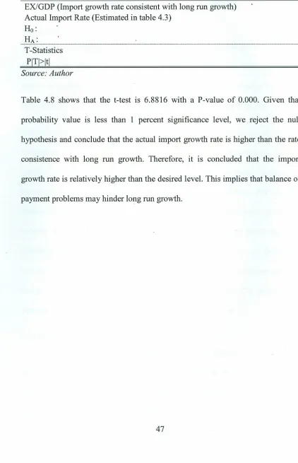
To address the second objective, the long run model, as provided in table 4.6 was used for analysis. Thirlwall hypothesized that the estimate of elasticity consistent with long run or balanced growth is estimated by the average volume of export as a ratio of GDP which is equal to 0.264. One sample test is used to compare the estimated income elasticity of imports (0.397) to the hypothesized long run rate of

Table 4.8: Test for Thirlwall's Hypothesis

Variable Name Mean Std. Err

EXlGDP

Actual Import Rate (Estimated in table 4.3)

Ho:

___:

t-!A_:

_

T-Statistics 6.8816

PITI>ltl 0.0000

Source: Author

0.0474

0.1015

Table 4.8 shows that the t-test is 6.8816 with a P-value of 0.000. Given that

probability value is less than 1 percent significance level, we reject the null

hypothesis and conclude that the actual import growth rate is higher than the rate

consistence with long run growth. Therefore, it is concluded that the import

growth rate is relatively higher than the desired level. This implies that balance of

CHAPTER FIVE

SUMMARY, CONCLUSION AND RECOMMENDATIONS

S.1.Summary

This study explored the effects of real exchange rate long run growth in Kenya.

The objectives adopted aimed at establishing the effect of real exchange rate on

current account balance in Kenya and secondly, to investigate whether the import

growth rate is consistent with the desired level of growth in the long run.

The study was pinned on neo classical elasticity approach and balance of payment

constraint model. Two models were estimated. The first model tested the Marshal

.Lerner condition while the later model tested Thirlwall's hypothesis. Annual time

series data from 1980 to 2011 was used for the investigation. The findings

revealed that GDP and Real exchange rate are major determinants of current

account balance changes. The findings further proved that Marshal-Lerner

Condition was applicable in the Kenyan economy. However, it was discovered

that the Thirlwall hypothesis was not supported by the data, it emerged that the

import growth rate in Kenya was significantly higher than the threshold as

asserted by Thirlwall' s hypothesis.

S.2.Conclusion

The main findings revealed that import is sensitive to changes in prices of imports

and exports. Secondly, estimated level of import elasticity of income is very high.

Responsiveness to import prices and high level of import growth rate is an

for exports in Kenya. In light of these findings, the following recommendations were made:

5.3.Recommendations

Firstly, high level of import demand is an indication of overreliance on imports in the country .. Therefore, the Kenyan government through its ministry of industrialization should introduce policies that will promote local production of quality goods and services to reduce demand for imported goods.

Secondly, given that Marshal-Lerner-Conditions holds, the central bank of Kenya should introduce measures to enforce the stability of Kenya shilling and create a

.conducive atmosphere for investment and growth. A stable currency may reduce volatility of import volume and thus help in solving the balance of payment issue.

Lastly, various arms of government should introduce policies that promote export led growth. Increase in export relative to imports will ensure promote rapid growth in demand and supply of goods and services across borders without deteriorating the economy's balance of payment position.

5.4 Limitations of the Study

REFERENCES

Britto G. and McCombie J. (2009).Thirlwall's Law and the long run equilibrium

growth rate. An Application to

Brazil.http://www.ppge.ufrgs.br/akb/encontros/2009/53.pdf [Viewed on

4th July 2013J

Dornbusch R. (1988) Open Economy Macroeconomics, 2nd Ed.New York:

Ghosh, A. and Ramakrishnan, U. (2006). Do Current Account Deficits Matter?

International Monetary

Fund.http://www.imf.org/external/pubs/ft/fandd/2006/12/basics.htm. [Vie

wed on

zs"

Johansen, S.(1998). Statistical Analysis of Co integrating Vectors. Journal of

EconomicDynamics and Control, Vol.12,pp.231-254.

Kariuki, G. (2009). Determinants of Current Account Balance in Kenya: The

Intertemporal approach. KIPPRA Discussion paper No. 93: KIPPRA.

Kenya-Official Exchange Rate. http://www.indexmundi.com/facts/kenya/

official-exchange-rate. [Viewed on 28th Apri12013J

Kenya -Current account Balance

http://www.indexmundi.com/facts/kenya/ current -account -balance

[Viewed on 28th Apri12013J

Kiptui, M and Kipyegon L. (2008) External Shocks and Real Exchange

Moreno-Brid, J. C. (2003). Capital Flows, Interest Payment and the Payment

and the Balance of Payments Constrained Growth Model.

Metroeconomica Vol. 54 No. 2-3 pp. 346-365

Mugenda, O. M. (2008). Research methods: quantitative and qualitative

approaches. Nairobi: Arts press.

Mudida (2012).Testing Marshal-Lerner condition inKenya.Brunell University

http://www.brunel.ac.uk/_data/assets/pdC file/0009/234279/1222.pdf

[Viewed on 3rd May 2013]

Musila J. and Rao, W. (200l).A Forecasting Model of the Kenyan

Economy.EconomicModelling.Vol. 19(1). Pp. 801-814

Ndung'u, N. (2001). Liberalization of the foreign exchange rate in Kenya and

short-term capital flow problems. The African Economic Research

Consortium. [Viewed on 26th April 2012]

Nusrate, A.(2008). The Role of Exchange Rate In Trade Balance.Empirical

evidence From Bangladesh. University of Birmingham, UK.

www.soegw.org/files/program/99-aziz.pdf[Viewed on 3rd May 2012]

Onafowara, D.A. (2003). Exchange Rate and Trade Balance in East Asia: Is There

a J-Curve? Economic Bulletin, Vol. 5,pp.l-13.

Ogwuru, H.(2008). Exchange Rate Dynamics and Current Account Balance in

Nigeria.