A NEW ALGORITHM FOR REMOVAL OF HIGH DENSITY SALT AND PEPPER NOISE IN MR IMAGES

(1)

A NEW ALGORITHM FOR REMOVAL OF HIGH

DENSITY SALT AND PEPPER NOISE IN MR IMAGES

Sumanta Saha

1

, Anindita Mohanta

2

, Sharmistha Bhattacharya (Halder)

3

1

Department of IT, Tripura University, Agartala, (India)

2

Department of IT, Tripura University, Agartala, (India)

3

Department of Mathematics, Tripura University, Agartala, (India)

ABSTRACT

Magnetic Resonance Images (MRI) are corrupted by impulsive noise mainly due to sensor faults of image

acquisition devices. This impulsive noise is most commonly referred to as “salt and pepper” noise. In this

article, a new approach has been introduced for removal of “salt and pepper” noise while preserving the image

details. This proposed method is basically a two-step method, wherein the first step; detect the corrupted pixel

since the impulse noise affects only certain pixels in the corrupted image and the remaining pixel values are

unchanged. In the second step, the corrupted pixel is replaced by the median value or by itsneighborhood

uncorrupted pixelvalueof the considering window. This proposed algorithm (PA) has shown encouraging

results, the Peak Signal to Noise Ratio (PSNR), Structured Similarity Index (SSIM) and Image Enhancement

Factor (IEF) of the filtered image using the PA are much higher values than the Wiener Filter (WF), Mean

Filter (MF), Standard Median Filter (SMF), Adaptive Median Filter (AMF)and other existing algorithms.

ThePA is also effective for other types of highly corrupted gray-scale and color images to remove

salt-and-pepper noise.

Keywords

-

De-noising, IEF, Impulse noise, Median filter, PSNR, Salt-and-Pepper noise, SSIM.

I. INTRODUCTION

Magnetic Resonance Images (MRI) are one of the most widely used medical imaging tools in both clinical and research applications [1]. The pixels in MR image, mainly gets corrupted due to the acquisition, bit errors in transmission and transformation process from analog to digital domain. In addition, images corrupted by these processes are mostly by the impulse noise. Also, impulse noise can be of two types namely, fixed valued impulse noise and random valued impulse noise [2]. Fixed valued impulse noise is also called as Salt and Pepper noise, which takes only two values either 0(Pepper) or 255(Salt), whereas random valued impulse noise can take any value between 0 and 255.

(2)

densities. Also it exhibits blurring if the window size is large and leads to insufficient noise suppression if the Window size is small [3]. In the case of the highly corrupted image, the edge details of the original image will not be preserved and blurring effect in the filtered image is one of the major drawbacks of SMF. During the filtering process of the corrupted image, it is importantthat the edge details have to be preserved. The perfect approach is to apply the filtering technique only to noisy pixels.

To remove SMF problems, Median filters such as Adaptive Median Filter (AMF), Decision–based median filters can be used for selecting the corrupted pixels first, and then apply the filtering technique on the corrupted pixel. As a result, only noisy pixels will be replaced by the median value and uncorrupted pixels will be left unchanged. AMF gives satisfactory performance at low noise densities since the corrupted pixels which are replaced by the median values are very few. Also, at higher noise densities, window size has to be increased to get better noise removal which will lead to less correlation between corrupted pixel values and replaced median pixel values. In the decision-based median filters, the decision is based on a pre-defined threshold value. However, the major drawback of Decision–based median filters is that defining a robust decision measure is difficult [3].

To overcome existing filtering problems, we proposed a new algorithm in this paper.This is consists of two stages. In the first stage, each pixel values are checked if a windows center pixel is corrupted and classify the corrupted and uncorrupted pixels. In the second stage, corrupted pixels are replaced by either the median pixel or neighborhood uncorrupted pixel. This proposed algorithm (PA) has used a fixed window size of 3×3 resulting in lower processing time compared with AMF and a smooth transition between the image pixels. Edge preservation, remove all noisy pixels and better visual quality have been observed from the results. Also, it gives better PSNR, SSIM and IEF values compared to the other filtering techniques like Mean Filter, Wiener Filter, Standard Median Filter [1], Adaptive Median Filter [4], [5], Decision Based Algorithm (DBA) [3], Modify Standard Median Filter (MMF) [1],and other existing algorithms[7], [8], [9], [10].

II.LITERATURE

REVIEW

Chan et al., [6] proposed an algorithm to overcome AMF problem, which consists of two stages. The first stage is to classify the corrupted and uncorrupted pixels by using AMF and in the second stage, regularization method is applied to the corrupted pixels to preserve edges and correct noisy pixels. Also, the drawback of this method is that for high impulse noise, it requires large window size of 39×39, so processing time is very high. Additionally, it requirescomplex circuitry for the implementation.

There are several approaches for identification and replacement of corrupted pixels butthe simplest approach is HanafyM.Ali [1] proposed algorithm. This algorithm consists of two stages. The first stage is to classify the corrupted and uncorrupted pixels and in the second stage, corrupted pixel is replaced by the median of its neighbors. However, the drawback of this method is that for high noise density, some noisy pixel values are left unchanged.

(3)

Esakkirajanet al. [7] proposed a Modified Decision Based Unsymmetrical Trimmed Median Filter (MDBUTMF) for the restoration of highly corrupted salt and pepper noise. In this algorithm, the noisy pixels is replaced by trimmed median value when other pixel values are 0’s and 255’s. When all pixel values are 0’s and 255’s, then the corrupted pixel is replaced by the mean value of all the elements present in the selected window. A.K. Samantarayet al. [8] proposed First Order Neighborhood DecisionBased Median Filter (FONDBMF) motivated by MDBUTMF filter. In this algorithm, the noisy pixels is replaced by the first order neighborhood pixels trimmed median value when other first order neighborhood pixel values are 0’s and 255’s. When all first order neighborhood pixel values are 0’s and 255’s, then the corrupted pixel is replaced by the mean value of the first order neighborhood pixels in the selected window.

Biswal, Satyabrata, and NilamaniBhoi[9]proposed a new method (NMF) for removal of high density salt and pepper noise. In this technique when the processing pixel is corrupted then its neighbors are checked. When all theneighbors are corruptedthen the processing pixel isreplaced with the mean value of the window. When some of the neighbors arecorrupted then processing pixel is replaced by the unsymmetric trimmed mean value. Aswini K Samantarayet al. [10] proposed a Decision Based Adaptive Neighborhood Median Filter (DBANMF).That is consists of three stages. In the first stage, it considers only the first order neighborhood (FON) pixels. In that if it finds one un-corrupted pixel, then that un-corrupted pixel replaces the corrupted center pixel. If it finds more than one corrupted pixel among the FON pixels, then the median value of those un-corrupted pixels replaces the un-corrupted center pixel. The second stage is followed by the first phase if and only if it does not find at least one un-corrupted pixel in the FON pixels. In the second stage, it considers only the diagonal neighborhood (DN) pixels. In DN if it finds only one un-corrupted pixel, then that un-corrupted pixel replaces the corrupted center pixel.And if it finds more than one un-corrupted pixel, then the median value of those un-corrupted pixels replaces the corrupted center pixel. If the method fails in above two phases i.e. if it does not find at least one un-corrupted pixel in its neighborhood, then it goes to the third phase. In this stage it calculates the mean of all the neighborhood pixels and replaces the corrupted center pixel by the calculated mean value.

III. SALT-AND-PEPPER

NOISE

An image containing salt-and-pepper noise will have dark pixels in bright areas and bright pixels in dark areas. Also, the negative impulse appears as black point (pepper noise) and the positive impulse appears as white point (salt noise) [1]. This type of noise can be caused by dead pixels, analog-to-digital converter errors, bit errors in transmission, fault memory locations in hardware or transmission in a noisy channel etc. This noise can be dark/bright pixels [11]. However, all pixels are not corrupted by salt and pepper noise in an image instead of some pixel values are changed and remaining pixels are unchanged. It is also known as fixed valued impulse noise and it is restricted to the minimum (0) or the maximum (255) intensity value [1]. The minimum intensity 0 appears as black pixels on the MR images. On the other hand, the maximum intensity 255 appears as white pixels on the MR images.

(4)

(1)

IV. PRELIMINARY

STUDY

Image de-noising is avery important task in image processing for the analysis of images. MR image de-noising methods can be linear as well as non-linear. Linear methods do not preserved the details of the images, whereas the non-linear methods preserved the details of the images. The non-linear filters like Median filter, provides good restoration from the noisy image [12]. It move filtering window over the noisy image and replace each center pixel by the median of the filtering window. The Median filter arecommonly used for removing impulse noise in MRI due to its good de-noisy property.

The standard median filter (SMF) is derived from the median filter.It attempts to remove noise by changing the center pixel value of the filtering window with the median of the neighbor’s pixel values. The median value is calculated by arranging all the neighbor’s pixel values in ascending order and select the middle pixel. SMF is very useful in salt -and-pepper noise filtering because they do not depend on values which are significantly different from the typical values in the neighborhood. The basic principal behind SMF is that the original pixel value, which is replaced by a newer one, that is closer to or the same as the median value eliminates isolated noise points [1]. However, the drawback of SMF is that itremoves thin lines and blurs image details even at medium noise densities. Also, the major drawback of SMF method is that it changed middle pixels value of selected 3x3 window without checking whether, it is corrupted or not.

There are several MRI image de-noising methods based on median filter like SMF, MMF [1] DBA [3], MDBUTMF [7], FONBDMF [8], NMF [9] and DBANMF [10], but they have the disadvantage of blurring edges. So, the aim of the new algorithm is to remove all corrupted pixel and maintaining reasonably edge of the MRI images even at the high noise density.

V. THE

PROPOSED

ALGORITHM

Median filters have chosen for removing salt-and-pepper noise because of their simplicity and less computational complexity. This paper describesa new decision based non-linear filteringtechnique for tackling the problem of median filters with minimal increase in computational load.Also, it preserved edges and restored all the noisy pixels. In most of the existing algorithms including SMF and AMF, only median values are used for the replacement of the corrupted pixels. The proposed de-noising algorithm (PA) is based on non-linear filtering technique. The PA first detects the salt and pepper noise in the image. The corrupted pixels in the image are detected by checking the pixel element value against the 0 and 255 values in the selected 3x3 window. Afterwards, inthe case of impulse noise corrupted pixel value is 0 or 255 and other values remain unchanged. In addition, this proposed algorithm (PA) consists of two stages. In the first stage, each pixel values are checked if a windows center pixel is corrupted and classify the corrupted and uncorrupted pixels. In the second stage, corrupted pixels are replaced by either the median pixel or neighborhood uncorrupted pixel. If the pixel have a value between 0 and 255 values in the 3x3 window of processing, then it is an uncorrupted pixel and any kind of changes are not required.

The steps of the proposed algorithm as follows:

(5)

Step 2.If 0< A2, 2 <255, then A2, 2 is an uncorrupted pixel.Its value is left unchanged and go to Step 7. Otherwise, A2, 2 is a noisy pixel.

Step 3.Find Wmin, Wmed and Wmax - the minimum, median and maximum pixel values respectively of W by

arranging the pixel values in ascending order.

Step 4.If A2, 2 is a noisy pixel, it will be replaced by Wmed, the median value of the W. Step 5.If Wmin=0 or Wmax =255, then read each pixel values of the W row wise.

Else go to Step 7.

Step 6.For each pixel Ax, yin the W do

If 0< Ax, y <255, then Ax, y is an uncorrupted pixel and its value is left unchanged. Otherwise Ax, y is a noisy pixel.

Case (i) If Ax, y is a noisy pixel and x=y=1 then Ax, y will be replaced by the right neighbor (A1, 2) pixel value, if the right neighbor pixel value is also noisy pixel then Ax, y will be replaced by the down neighbor (A2, 1) pixel value, if the down neighbor pixel value is also noisy then Ax, y will be replaced by A2, 2.

Case (ii)If Ax, y is a noisy pixel, where x ≠ y and y=2, then Ax, y will be replaced by the right neighbor pixel

value, if the right neighbor pixel value is also noisy pixel then Ax, y will be replaced by the left neighbor pixel value.

Case (iii) If Ax, y is a noisy pixel, x ≠ y and x=2 then Ax, y will be replaced by the down neighbor pixel value,

if the down neighbor pixel value is also noisy pixel then Ax, y will be replaced by the right/left neighbor (A2, 2) pixel value.

Case (iv)If Ax, y is a noisy pixel, where x =1 and y= 3 then Ax, y will be replaced by the down neighbor (A2, 3) pixel value, if the down neighbor pixel value is also noisy then Ax, y will be replaced by the left neighbor (A1, 2) pixel value.

Case (v)If Ax, y is a noisy pixel, where x =3 and y= 1 then Ax,y will be replaced by the right neighbor (A3, 2) pixel value, if the right neighbor pixel value is also noisy pixel then Ax, y will be replaced by the upper neighbor (A2, 1) pixel value.

Step 7. Repeat Steps 1 to 6 until all the pixels in the entire image are processed.

In the PA, the nature of the pixel being processed first, that is, it is corrupted or not, is checked. The value of the pixel being processed is then replaced with the corresponding value as in Step 4 and cases (i), (ii), (iii), (iv), (v) of Step 6. The window is then subsequently moved to form a new set of values. This process is repeated until the last image pixel is processed.

VI. METHODOLOGY

OF

THE

PROPOSED

ALGORITHM

Consider a 3x3 window:

P1 P2 P3 P4 P5 P6

P7 P8 P9

(6)

Case1:If P5 is corrupted pixel then P5 is replaced by the median pixel value of the selected 3x3 window and checked its neighborP1, P2, P3, P4, P6, P7 and P8 pixels are corrupted or not respectively. Else select the next window and repeat case1.

Case2:If P1is a corrupted pixel then itis replaced by P2if P2 is also corrupted pixel then P1 is replaced by P4 if

P2 and P4 both are corrupted pixelsthen P1 is replaced by P5. Here, P5 is already processed pixel, so no need to

check.

Case3:IfP2 pixel is corrupted then it is replaced by P3if P3 is also corrupted pixel then P2 is replaced by P1.

Here, P1 is already processed pixel values so no need to check.

Case4: If P3 pixel is corrupted then it is replaced by P6 if P6 is also corrupted pixel then P3 is replaced by P2.

(Note: P9 pixel value is not checked, if P9 is corrupted then P9 is correct at subsequent window moves on the image.)

Consider a corrupted 8x5 windows pixel values of an image. Modification of corruptedpixels using the PA is shown inFig.1.

(A) (B) (C)

(D) ( E)

(7)

VII. IMAGE

QUALITY

ASSESSMENT

The performance of the de-noising process is measured by the Peak Signal-to-Noise Ratio (PSNR), Structured Similarity Index (SSIM) and Image Enhancement Factor (IEF). The PSNR, SSIM and IEF can be viewed as a quality measure of one of the images being compared, provided the other image is regarded as of perfect quality. Larger PSNR, SSIM and IEF indicate a minor difference between the original image and the filtered image. The mean squared error (MSE) is defined for an image as [13] :

(2) Where, A is the original image, I is the restored image and size of the image is m×n.

PSNR is the most widely used objective image quality/distortion measure [14]. The following equation describes the PSNR [2],[15] :

(3)

Where, MAX is the maximum possible pixel value of an image that is 255.

The Structural Similarity (SSIM) index is a novel technique for measuring the similarity between two images. It is an improved version of the Universal Image Quality Index (UIQI).Structural similarity provides an alternative and complementary approach to the problem of image quality assessment. The following equation describes the SSIM [3]:

(4)

, ,

G=255; K1, K2<<1, (K1=0.001, K2=0.002) The following equation describes the IEF [3] :

(5) where, Ois the original Image, R is the restored image, P is the corrupted image, m×nis the size of the image, L is the luminance comparison, C is the contrast comparison, S is the structure comparison, μ is the mean and σ is the standard deviation.

The PSNR, SSIM and IEF are computed for purposes of comparison.To validate the proposed scheme, simulation has been carried out in MATLAB (r2009a) on standard MR images.

VIII. RESULTS

OF

THE

PROPOSED

ALGORITHM

(8)

densities. Then PA is applied to the corrupted image to remove the noise. The sample MRI images considered during the experimental process is shown in Fig. 2(A) – Fig. 2(D). The de-noising of MR images corrupted by salt-and-pepper noise at different noise density are shown in Fig. 3(A) – Fig. 3(F).

(A) (B)

(C) (D)

Fig. 2.The Original MRI images (A) Kidney, (B) Liver, (C)Sectional View of the Brain, (D) Back view of the Brain.

(A)

(B)

(9)

(D)

(E)

(F)

Fig. 3.(A) 25% Salt and pepper Noise density and Restored Image of Kidney; (B) 65% Salt and pepper Noise

density and Restored Image of Liver; (C) 85% Salt and pepper Noise density and Restored Image of Liver; (D) 90% Salt and pepper Noise density and Restored Image of Sectional View of the Brain; (E) 93% Salt and pepper Noise density and Restored Image of Sectional View of the Brain; (F) 96% Salt and pepper Noise density and Restored Image of Back view of the Brain.

IX. COMPARISON

(10)

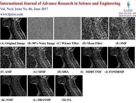
sample MR images considered during the experimental process is shown in Fig.4(A), Fig.6(A), and Fig.8(A).The comparative analysisof different de-noising algorithms of MR images corrupted by salt-and-pepper noise at 90%dB noise density is shown in Fig.4, Fig. 6, and Fig. 8.

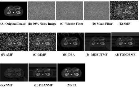
(A) Original Image (B) 90% Noisy Image (C) Wiener Filter (D) Mean Filter (E) SMF

(F) AMF (G) MMF (H) DBA (I) MDBUTMF (J) FONDBMF

(K) NMF (L) DBANMF (M) PA

Fig. 4.Comparative analyses of Noise removal techniques for Kidney MRI in 90% Salt and pepper Noise density.

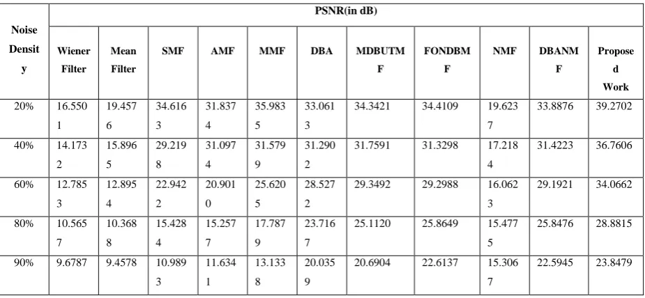
Table.I. PSNR Values for Kidney MRI with Different Noise Densities.

Table.II. Noise Densit y PSNR(in dB) Wiener Filter Mean Filter

SMF AMF MMF DBA MDBUTM

F

FONDBM

F

NMF DBANM

F

Propose

d

Work

20% 15.195

7 17.839 0 30.424 2 30.846 3 32.747 4 31.983 1

24.5818 20.4361 21.360

6

23.6471 40.9367

40% 12.477

6 13.308 5 26.752 8 33.157 1 28.295 8 28.755 4

24.0284 20.3253 20.574

9

23.2866 36.0589

60% 10.191

9 10.470 0 21.692 3 19.602 4 22.768 2 26.451 7

22.9961 19.9512 20.064

2

22.6349 32.5678

80% 8.2577 8.3687 14.487

7 12.998 8 15.082 6 23.498 8

21.4280 19.2747 19.553

5

21.5397 28.6285

90% 7.4097 7.4568 9.7477 8.5779 10.315

8

19.555

2

18.8884 18.5227 19.161

7

(11)

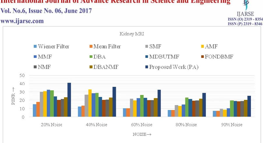
Fig. 5.PSNR Performance of various algorithms over Kidney MRI corrupted by salt and pepper noise.

Table.III. SSIM for Kidney MRI with Different Noise Densities.

Noise

Density

SSIM

Wiener

Filter

Mean

Filter

SMF AMF MMF DBA MDBUTMF FONDBMF NMF DBANM

F

Proposed

Work

20% 0.1010 0.1202 0.8994 0.9540 0. 9703 0.8852 0.5924 0.5924 0.3637 0.5262 0.9699

40% 0.0555 0.0615 0.8166 0.9593 0. 9188 0.8680 0.5694 0.5784 0.3322 0.5463 0.9470

60% 0.0354 0.0374 0.5728 0.6899 0. 6858 0.8205 0.4506 0.4912 0.3054 0.5054 0.9194

80% 0.0217 0.0210 0.1589 0.4001 0. 2164 0.6648 0.3292 0.4582 0.2718 0.4336 0.8489

90% 0.0157 0.0168 0.0405 0.2329 0. 0647 0.3916 0.2359 0.3555 0.2440 0.2801 0.7387

Table.IV. IEF for Kidney MRI with Different Noise Densities.

Noise

Densit

y

IEF

Wiener

Filter

Mean

Filter

SMF AMF MMF DBA MDBUTMF FONDBMF NMF DBANMF Proposed

Work

20% 0.9597 1.7607 21.042 32.2438 56.1639 28.0905 5.4808 2.1100 2.6105 4.4196 356.6682

40% 0.5140 0.6260 9.1071 58.3219 19.9338 14.3100 4.8188 2.0542 2.1757 4.0623 118.1964

60% 0.3073 0.3275 2.8104 2.0549 5.5389 8.4080 3.7945 1.8821 1.9317 3.4915 54.9869

80% 0.1967 0.2000 0.5342 0.4825 0.9168 4.2545 2.6410 1.6085 1.7152 2.7097 21.5740

(12)

(F) AMF (G) MMF (H) DBA (I) MDBUTMF (J) FONDBMF

(K) NMF (L) DBANMF (M) PA

Fig. 6.Comparative analyses of Noise removal techniques forlateral view of the Brain MRI in 90% Salt and pepper Noise density.

Table.V. PSNR Values for Lateral View of the Brain MRI with Different Noise Densities.

Noise Densit y PSNR(in dB) Wiener Filter Mean Filter

F

FONDBM

F

NMF DBANM

F

Propose

d

Work

20% 16.550

1 19.457 6 34.616 3 31.837 4 35.983 5 33.061 3

34.3421 34.4109 19.623

7

33.8876 39.2702

40% 14.173

2 15.896 5 29.219 8 31.097 4 31.579 9 31.290 2

31.7591 31.3298 17.218

4

31.4223 36.7606

60% 12.785

3 12.895 4 22.942 2 20.901 0 25.620 5 28.527 2

29.3492 29.2988 16.062

3

29.1921 34.0662

80% 10.565

7 10.368 8 15.428 4 15.257 7 17.787 9 23.716 7

25.1120 25.8649 15.477

5

25.8476 28.8815

90% 9.6787 9.4578 10.989

3 11.634 1 13.133 8 20.035 9

20.6904 22.6137 15.306

7

(13)

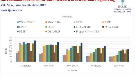
Fig. 7.PSNR Performance of various algorithms over lateral view of the Brain MRI corrupted by salt and pepper noise.

Table.VI. SSIM for Lateral View of the Brain MRI with Different Noise Densities.

Noise

Density

SSIM

Wiene

r Filter Mean

Filter

SMF AMF MMF DBA MDBUTMF FONDBM

F

NMF DBANM

F

Proposed

Work

20% 0.1466 0.2153 0.9831 0.9538 0.9970 0.9897 0.9779 0.9750 0.5341 0.9751 0.9975

40% 0.0879 0.1114 0.9064 0.4870 0.9755 0.9801 0.9689 0.9627 0.5045 0.9629 0.9825

60% 0.0590 0.0687 0.6464 0.7160 0.7848 0.9385 0.9422 0.9367 0.5261 0.9367 0.9595

80% 0.0410 0.0452 0.2273 0.4518 0.3533 0.8147 0.8682 0.8713 0.5871 0.8709 0.8863

90% 0.0338 0.0369 0.0795 0.2393 0.1335 0.6953 0.7794 0.7882 0.6410 0.7879 0.7932

Table.VII. IEF for Lateral View of the Brain MRI with Different Noise Densities.

Noise

Density

IEF

Wiener

Filter

Mean

Filter

SMF AMF MMF DBA MDBUTMF FONDB

MF

NMF DBANMF Proposed

Work

20% 4.6008 8.9613 294.3830 153.4624 396.8069 205.786 276.3710 280.7859 9.3251 248.9122 876.8195

40% 2.6430 3.4256 84.9393 7.9875 140.2624 136.819 152.4166 138.0722 5.3576 141.0450 522.7693

60% 1.6800 1.8476 20.0072 12.2499 36.6455 72.3919 87.4782 86.4659 4.1039 84.3693 113.7744

80% 1.1260 1.1606 3.5453 3.4610 6.2984 23.9047 32.9621 39.2021 3.5856 39.0459 49.5144

(14)

(F) AMF (G) MMF (H) DBA (I) MDBUTMF (J) FONDBMF

(K) NMF (L) DBANMF (M) PA

Fig. 8.Comparative analyses of Noise removal techniques for Spine MRI in 90% Salt and pepper Noise density.

Fig. 9.

Table.VIII. PSNR Values for Spine MRI with Different Noise Densities.

Noise Density

PSNR(in dB)

Wiener Filter

Mean Filter

SMF AMF MMF DBA MDBUTMF FONDBMF NMF DBANMF Proposed

Work

20% 15.7868 18.7966 31.2038 31.7787 33.7678 33.4819 34.0545 32.8670 23.3264 33.2116 36.0860

40% 13.2789 14.9665 27.0891 32.9764 30.7686 29.9418 29.9038 29.1834 20.7021 29.3794 33.2285

60% 11.1679 11.9765 21.7707 20.1435 24.4694 27.1076 26.9666 26.5197 19.6197 26.5764 30.6918

80% 9.2905 9.8906 14.7292 14.8227 17.9675 23.5782 22.9508 23.1175 19.0168 23.0791 26.6784

90% 8.7864 8.9064 10.4517 11.6789 12.3146 20.8385 19.7741 20.6477 18.7891 20.4619 22.7890

(15)

Table.IX. SSIM for Spine MRI with Different Noise Densities.

Noise Densit y

SSIM

Wiene r Filter

Mean Filter

SMF AMF MMF DBA MDBUT

MF

FONDB MF

NMF DBANMF Propose

d Work

20% 0.1807 0.2445 0.9520 0.9574 0. 9920 0.9924 0.9936 0.9914 0.8059 0.9913 0.9897

40% 0.1078 0.1261 0.8723 0.5398 0. 9574 0.9727 0.9738 0.9656 0.7705 0.9661 0.9695

60% 0.0680 0.0763 0.6361 0.7348 0. 7922 0.9226 0.9248 0.9127 0.7623 0.9141 0.9429

80% 0.0393 0.0419 0.2381 0.4716 0. 3807 0.8042 0.8119 0.8051 0.7555 0.8030 0.8478

90% 0.0287 0.0314 0.0872 0.2814 0. 1540 0.6958 0.7017 0.6996 0.7357 0.6927 0.7215

IEF for Spine MRI with Different Noise Densities.

Noise Densit y

IEF

Wiener Filter

Mean Filter

F

FONDBMF NMF DBANM

F

Propose d Work

20% 1.9883 3.7994 67.6807 69.7236 113.5984 114.366 130.4805 99.2672 11.034 107.4602 138.5915

40% 1.1008 1.3749 26.2189 3.2919 45.1715 50.5706 50.1283 42.4656 6.0245 44.4259 83.9790

60% 0.6793 0.7317 7.6981 5.5893 14.0765 26.3072 25.4667 22.9762 4.6912 23.2791 51.8682

80% 0.4433 0.4561 1.5200 1.5231 2.6178 11.6619 10.0926 10.4875 4.0793 10.3943 20.2124

90% 0.3679 0.3725 0.5674 0.6982 0.9246 6.2025 4.8547 5.9361 3.8694 5.6873 8.5629

X. CONCLUSION

In this paper, we have introduced a new and effective filtering method for Salt and Pepper noise which is strong to various noise levels. The PA detect the corrupted pixel first, since the impulse noise only affect certain pixels in the image and remaining pixels are unchanged. The proposed filter compared with the traditional filtering techniques (mean filter, wiener filter, and standard median filter) and other existingfiltering (AMF, MMF, DBA, MDBUTMF, FONDBMF, NMF, and DBANMF) techniques.Experimental results indicate that this proposed filtering algorithm(PA) can reduce salt and pepper noise effectively and maintain details of the MR images in comparison with other noise removal algorithms in terms of PSNR, SSIM and IEF.

REFERENCES

[1] Ali, Hanafy M. "A new method to remove salt & pepper noise in Magnetic Resonance Images." Computer Engineering & Systems (ICCES), 2016 11th International Conference on. IEEE, 2016.

(16)

[3] Nair, Madhu S., K. Revathy, and RaoTatavarti. "Removal of salt-and pepper noise in images: a new decision-based algorithm." Proceedings of the International Multi Conference of Engineers and Computer Scientists. Vol. 2. 2008.

[4] Leavline, E. Jebamalar, and D. Asir Antony Gnana Singh. "Salt and pepper noise detection and removal in gray scale images: an experimental analysis." International Journal of Signal Processing, Image Processing and Pattern Recognition 6.5 (2013): 343-352.

[5] Bhatia, A. N. I. S. H. A. "Decision based median filtering technique to remove salt and pepper noise in images." Proc. of international conference on ITR. Bhubaneswar, 2013.

[6] Chan, Raymond H., Chung-Wa Ho, and Mila Nikolova. "Salt-and-pepper noise removal by median-type noise detectors and detail-preserving regularization." IEEE Transactions on image processing 14.10 (2005): 1479-1485.

[7] Esakkirajan, S., et al. "Removal of high density salt and pepper noise through modified decision based unsymmetric trimmed median filter." IEEE Signal processing letters 18.5 (2011): 287-290.

[8] Samantaray, Aswini Kumar, and PriyadarshiKanungo. "First order neighborhood decision based median filter." Information and Communication Technologies (WICT), 2012 World Congress on. IEEE, 2012. [9] Biswal, Satyabrata, and NilamaniBhoi. "A new filter for removal of salt and pepper noise." Signal

Processing Image Processing & Pattern Recognition (ICSIPR), 2013 International Conference on. IEEE, 2013.

[10] Samantaray, Aswini Kumar, and PriyankaMallick. "Decision Based Adaptive Neighborhood Median Filter." Procedia Computer Science 48 (2015): 222-227.

[11] MalothuNagu, N. VijayShanker. "Image De-Noising By Using Median Filter and Weiner Filter." International Journal of Innovative Research in Computerand Communication Engineering 2.9 (2014). [12] Chandel, Ruchika, and Gaurav Gupta. "Image Filtering Algorithms and Techniques: A Review."

International Journal of Advanced Research in Computer Science and Software Engineering 3.10 (2013). [13] Kaur, Pardeep, and ManinderKaur. "Decision Based Trimmed Adaptive Windows Median Filter."

International Journal of Science and Research 6 (2013): 40-43.

[14] Leavline, E. Jebamalar, and S. Sutha. "Gaussian noise removal in gray scale images using fast Multiscale Directional Filter Banks." Recent Trends in Information Technology (ICRTIT), 2011 International Conference on. IEEE, 2011.