Effects of Regional Climate Model Spatial Resolution on
Hydrological Modelling of Summer-Fall Floods
in Southern Quebec
by
Mariana CASTANEDA-GONZALEZ
THESIS PRESENTED TO ÉCOLE DE TECHNOLOGIE SUPÉRIEURE
IN PARTIAL FULFILLMENT FOR A MASTER’S DEGREE WITH THESIS
IN ENVIRONMENTAL ENGINEERING
M. A. Sc.
MONTREAL, JANUARY 24
TH, 2018
ÉCOLE DE TECHNOLOGIE SUPÉRIEURE
UNIVERSITÉ DU QUÉBEC
This Creative Commons licence allows readers to download this work and share it with others as long as the author is credited. The content of this work can’t be modified in any way or used commercially.
BOARD OF EXAMINERS
THIS THESIS HAS BEEN EVALUATED BY THE FOLLOWING BOARD OF EXAMINERS
Mr. Richard Arsenault, Eng., Ph.D., Thesis Supervisor
Département du génie de la construction at École de technologie supérieure
Mr. Rabindranarth Romero-Lopez, Eng., Ph.D., Thesis Co-supervisor Civil engineering department at the University Veracruzana
Ms. Danielle Monfet, Eng. Ph.D., President of the Board of Examiners Département du génie de la construction at École de technologie supérieure
Mr. François Brissette, Eng. Ph.D., Member of the jury
Département du génie de la construction at École de technologie supérieure
THIS THESIS WAS PRENSENTED AND DEFENDED
IN THE PRESENCE OF A BOARD OF EXAMINERS AND PUBLIC MONTREAL, DECEMBER 19TH, 2017
ACKNOWLEDGMENTS
I am very grateful for all the support I have received since the very first day I arrived in Montreal. Without the constant help from so many people it would not have been the great experience that it has been
This thesis has been the result of the great support provided by the École de Technologie Supérieure, providing me the guidance and access to everything necessary for the realization of this thesis. Likewise, I am very grateful for the support provided for all the members of the DRAME. It has been an unforgettable experience to have shared many hours together. I feel very lucky for having found this amazing group of people. And I look forward to keep working together and to share new moments with you all.
I am very grateful to my supervisor, Annie Poulin. Your constant support and guidance was fundamental to complete this thesis. I thank also my co-supervisor, Rabindranarth, for all the help and time you dedicated for this thesis.
Special thanks to Richard Arsenault and François Brissette. Your help and guidance during these last months has been invaluable. I feel privileged and lucky to have had the opportunity of working with you.
I thank the great support provided from the Ouranos Consortium and the Ministère du Développement Durable, de l’Environnement et de la Lutte contre les Changements Climatiques (MDDELCC). Your expertise was fundamental during all the process of my studies. I also thank the Consejo Nacional de Ciencia y Tecnologia (CONACYT) for providing the financial support to pursue my graduate studies.
And finally, it is difficult to express the great gratitude to my parents and siblings for always encouraging me and support me at all times. Despite the distance, you have always supported
me in the same way. You were always there whenever I needed, unconditionally. Esta tesis es dedicada a ustedes.
EFFETS DE LA RÉSOLUTION SPATIALE D'UN MODÈLE CLIMATIQUE RÉGIONAL SUR LA MODÉLISATION HYDROLOGIQUE DES CRUES
D'ÉTÉ-AUTOMNE DANS LE SUD DU QUÉBEC.
Mariana CASTANEDA-GONZALEZ
RÉSUMÉ
Cette étude vise à évaluer les effets de la résolution spatiale du Modèle Régional Canadien du Climat (MRCC) sur la simulation des crues d'été et d'automne. Sept différentes simulations climatiques issues de la quatrième et de la cinquième version du MRCC sont utilisées. Les quatre simulations climatiques issues de la quatrième version du MRCC sont comparées. Elles consistent de deux simulations pilotées par le Modèle Canadien de Circulation Général (MCCG) et deux par la réanalyse ERA-40c, chacune à des résolutions différentes de 15 km et 45 km. Les trois simulations climatiques issues de la cinquième version du MRCC sont pilotées par la réanalyse ERA-Interim à des résolutions spatiales de 0,44 ° (≈ 48 km), 0,22 ° (≈ 24 km) et 0,11 ° (≈ 12 km). Toutes les comparaisons sont évaluées sur un pas de temps journalier pour les périodes de 1961-1990 (pour le MRCC4) et de 1981-2010 (pour le MRCC5).
Les sept simulations sont utilisées comme données d'entrée pour deux modèles hydrologiques de complexité variable (HSAMI et MOHYSE). Chaque modèle est calibré en utilisant trois fonctions-objectifs basées sur le critère d’efficience Kling-Gupta Efficiency (KGE) pour cibler les crues d’été-automne. Trois indices saisonniers sont utilisés pour évaluer les sorties du MRCC : biais (température), biais relatif (précipitations) et le ratio de variances (température et précipitations). Dans le but d'évaluer les effets de la résolution spatiale sur la modélisation hydrologique des crues d’été-automne, des simulations d'écoulement sont générées à l'aide des sept jeux de données climatiques. Les simulations d'écoulement générées par les sorties climatiques sont analysées par deux statistiques de performance : les KGE saisonniers et les biais relatifs saisonniers. Les crues d’été-automne sont évaluées à l'aide de quatre indicateurs de crue, soient les périodes de retour de 2, 5, 10 et 20 ans.
Les résultats ont révélé un impact de la résolution spatiale sur les sorties du MRCC (température et précipitation) et sur la simulation des crues d’été-automne par les deux modèles hydrologiques et les trois différentes approches de calage, bien que cela puisse être dû à d'autres éléments tels que la taille du domaine et le choix du pilote du modèle climatique. En augmentant la résolution spatiale pour les deux modèles hydrologiques, les indicateurs de crue d’été-automne affichent une augmentation des périodes de retour. D'autre part, la structure des modèles hydrologiques et les approches de calage n'ont pas montré d'impacts significatifs sur les simulations des crues d’été-automne. Les résultats soulignent la nécessité de poursuivre des études pour évaluer l'incertitude supplémentaire due aux impacts de la résolution spatiale des simulations climatiques sur les études hydrologiques.
EFFECTS OF REGIONAL CLIMATE MODEL SPATIAL RESOLUTION ON HYDROLOGICAL MODELLING OF SUMMER-FALL FLOODS IN SOUTHERN
QUEBEC.
Mariana CASTANEDA-GONZALEZ
ABSTRACT
This study aims to evaluate the effects of the Canadian Regional Climate Model’s (CRCM) spatial resolution on summer-fall floods simulation. Seven different climate simulations issued from the fourth and the fifth version of the CRCM are employed. Four different climate simulations issued from the fourth version of the CRCM (CRCM4) are compared. They are composed of two simulations driven by the Canadian General Circulation Model (CGCM) and two driven by the ERA-40c reanalysis using grid meshes of 15 km and 45 km resolutions for each driver. Three climate simulations issued from the fifth version of the CRCM (CRCM5) driven by the ERA-Interim at 0.44° (≈ 48 km), 0.22° (≈ 24 km) and 0.11° (≈ 12 km) spatial resolutions are used. All comparisons are evaluated on a daily time-step for the 1961-1990 period (for CRCM4) and for the 1981-2010 period (for CRCM5).
These seven simulations (four from CRCM4 and three from CRCM5) are used as input for two hydrological models of varying complexity (HSAMI and MOHYSE). Each model is calibrated using three different objective functions based on the Kling-Gupta Efficiency criteria (KGE) to target the summer-fall floods. Three seasonal indices are used to evaluate the CRCM outputs: bias (temperature), relative bias (precipitation) and variances ratio (temperature and precipitation). In an attempt to evaluate the effects of the spatial resolution on the hydrological modelling of summer-fall floods, streamflow simulations are generated using the seven climate datasets. The generated climate-driven streamflow simulations are analysed by two performance statistics: the seasonal values of KGE and the seasonal relative biases. Summer-fall floods are evaluated through the use of four flood indicators, the 2-year, 5-year, 10-year and 20-year return periods
The results revealed an impact of spatial resolution on climate model outputs (temperature and precipitation) and on summer-fall floods simulation by the two hydrological models and the three different calibration approaches, although this can be due to other elements such as domain size and climate model driver. The flood indicators demonstrate an increase on the summer-fall floods return periods with increasing resolution from both hydrological models. On the other hand the hydrological models structure and the calibration approaches did not show significant impacts on the summer-fall floods. The results highlight the need for further research to assess the additional uncertainty due to the impacts of the climate simulations spatial resolution on hydrological studies.
TABLE OF CONTENTS
Page
INTRODUCTION ...1
CHAPTER 1 LITERATURE REVIEW ...3
1.1 Floods and future trends...3
1.2 Hydrological modelling ...4
1.2.1 Calibration and validation process ... 5
1.3 Global and regional climate modelling ...7
1.3.1 Climate projections: general trends ... 11
1.3.2 Sources of uncertainty... 13
1.4 Regional studies: Quebec ...14
1.5 Research objectives ...16
CHAPTER 2 STUDY AREA AND DATA ...17
2.1 Study area...17
2.2 Observed data ...18
2.3 Climate simulation data ...19
2.3.1 Regional climate model (RCM) ... 20
CHAPTER 3 METHODS ...21
3.1 Overview ...21
3.2 Climate data comparison ...22
3.3 Hydrological modelling ...24
3.3.1 Hydrological models ... 25
3.3.2 Calibration and validation ... 25
3.3.3 Streamflow simulations ... 26
3.3.3.1 Return Periods ... 28
CHAPTER 4 RESULTS ...29
4.1 Climate simulations intercomparison ...29
4.1.1 Spatial resolution ... 29
4.1.1.1 Temperature ... 29
4.1.1.2 Precipitation ... 34
4.2 Hydrological modelling performance ...38
4.2.1 HSAMI and MOHYSE calibration and validation results ... 38
4.2.1.1 Spatial distribution of hydrological modelling performance ... 40
4.2.1.2 Hydrological model parameter sets ... 43
4.3 Climate model driven streamflow simulations ...45
4.3.1 Spatial resolutions ... 45
4.3.2 Hydrological model parameter sets ... 48
CHAPTER 5 DISCUSSION ...51
5.2 Climate model-driven hydrological streamflow simulations ...54
5.2.1 Generation of the climate model-driven hydrological streamflows ... 54
5.2.2 Spatial resolution effects on climate model-driven hydrological streamflows ... 55
5.2.3 Flood indicators ... 56
5.3 Hydrological models structure and parameters impacts ...56
5.4 Regional climate model configuration ...57
5.5 Streamflow simulations and catchment size ...60
5.6 Limitations ...62
CONCLUSION ...65
RECOMMENDATIONS ...69
APPENDIX I REGIONAL CLIMATE MODEL DOMAINS ...71
APPENDIX II CLIMATE SIMULATIONS INTERCOMPARISON: DRIVERS ...73
APPENDIX III STREAMFLOW SIMULATIONS AND CATCHMENT SIZE ...75
LIST OF TABLES
Page Table 1.1 Trends for the 2050 horizon for southern Quebec. ... 15 Table 2.1 Description of the CRCM climate datasets used in this study ... 19 Table 3.1 Summary of CRCM4 and CRCM5 climate datasets comparisons ... 22 Table 3.2 Summary of the objective functions for the hydrological model’s
LIST OF FIGURES
Page Figure 1.1 Hydrological modelling calibration process ... 6 Figure 1.2 Mean summer maximum temperature for the reference period 1970–
1999 from observations (E-OBS v5.0 0.5◦(Haylock et al., 2008)) and a range of AOGCMs in the CMIP3 database. Taken from Hawkins et al. (2013, p. 20) ... 9 Figure 1.3 Regional climate model configuration ... 10 Figure 1.4 Cascade of uncertainty ... 14 Figure 2.1 Location and mean annual precipitation (mm) of the 50 watersheds
used in this study ... 17 Figure 3.1 Overview of this project’s research methodology ... 21 Figure 4.1 Annual daily mean temperature (°C) bias between simulations issued
from CRCM4 for the summer (JJA) and fall (SON) seasons for the period 1961-1990.The upper panels (a) show the comparisons for the datasets driven by CGCM. The lower panels (b) show the comparisons for the datasets driven by ERA40c ... 30 Figure 4.2 Annual daily mean bias of temperature (°C) between simulations
issued from CRCM5 for the summer (JJA) and fall (SON) seasons for the period 1981-2010.The upper panels (a) show the comparisons for the datasets with 12 km and 24 km resolution. The lower panels (b) show the comparisons for the datasets with 12 km and 48 km resolution... 31 Figure 4.3 Ratio of annual seasonal mean temperature variances between
simulations issued from CRCM4 for the summer (JJA) and fall (SON) seasons for the period 1961-1990.The upper panels (a) show the comparisons for the datasets driven by CGCM. The lower panels (b) show the comparisons for the datasets driven by ERA40c ... 32 Figure 4.4 Ratio of annual seasonal mean temperature variances between
simulations issued from CRCM5 for the summer (JJA) and fall (SON) seasons for the period 1981-2010. The upper panels (a) show the comparisons for the datasets with 12 km and 24 km resolution. The lower panels (b) show the comparisons for the datasets with 12 km and 48 km resolution ... 33
Figure 4.5 Annual daily mean relative precipitation biases (%) between simulations issued from CRCM4 for the summer (JJA) and fall (SON) seasons for the period 1961-1990.The upper panels (a) show the comparisons for the datasets driven by CGCM. The lower panels (b) show the comparisons for the datasets driven by ERA40c ... 34 Figure 4.6 Annual daily mean relative biases (%) of precipitation between
simulations issued from CRCM5 for the summer (JJA) and fall (SON) seasons for the period 1981-2010. The upper panels (a) show the comparisons for the datasets with 12 km and 24 km resolution. The lower panels (b) show the comparisons for the datasets with 12 km and 48 km resolution ... 35 Figure 4.7 Ratio of annual seasonal mean temperature variances between
simulations issued from CRCM4 for the summer (JJA) and fall (SON) seasons for the period 1961-1990. The upper panels (a) show the comparisons for the datasets driven by CGCM. The lower panels (b) show the comparisons for the datasets driven by ERA40c ... 36 Figure 4.8 Ratio of annual seasonal mean temperature variances between
simulations issued from CRCM5 for the summer (JJA) and fall (SON) seasons for the period 1981-2010. The upper panels (a) show the comparisons for the datasets with 12 km and 24 km resolution. The lower panels (b) show the comparisons for the datasets with 12 km and 48 km resolution ... 37 Figure 4.9 KGE values on the calibration and validation years. Panel a) presents
the objective function-1, b) the objective function-2 and c) presents the objective function-3. KGE values for all the year (left panel) and June to October (right panel) are shown for both models and each objective function... 39 Figure 4.10 Map of the KGE values on the validation years with the OF-1 over
the fifty watersheds. The upper panels (a) present the performances over the full time series and the lower panels (b) present the performances during summer-fall months (June-October) ... 40 Figure 4.11 Map of the KGE values on the validation years with the OF-2 over
the fifty watersheds. The upper panels (a) present the performances over the full time series and the lower panels (b) present the performances during summer-fall months (June-October) ... 41 Figure 4.12 Map of the KGE values on the validation years with the OF-2 over
the fifty watersheds. The upper panels (a) present the performances over the full time series and the lower panels (b) present the performances during summer-fall months (June-October) ... 42
Figure 4.13 KGE values of the 50 watersheds for the different calibration approaches on the calibration years. The upper panels (a) present the KGE values for the full-time series and the lower panels (b) present the values for the summer-fall months... 43 Figure 4.14 KGE values of the 50 watersheds for the different calibration
approaches on the validation years. The upper panels (a) present the KGE values for the full-time series and the lower panels (b) present the values for the summer-fall months... 44 Figure 4.15 Seasonal KGE values of the comparisons between streamflows
generated with climate outputs at different resolutions. The upper panels (a) present the results obtained with OF-1, the middle panels (b) present the results obtained with OF-2 and the lower panels (c) present the results obtained with OF-3 ... 45 Figure 4.16 Seasonal relative bias values of the comparisons between
streamflows generated with climate outputs at different resolutions. The upper panels (a) present the results obtained with OF-1, the middle panels (b) present the results obtained with OF-2 and the lower panels (c) present the results obtained with OF-3 ... 46 Figure 4.17 Relative biases (%) between the return periods (2, 5, 10 and 20-year)
of the different generated streamflows. The upper panels (a) present the results obtained with OF-1, the middle panels (b) present the results obtained with OF-2 and the lower panels (c) present the results obtained with OF-3 ... 47 Figure 4.18 KGE values between generated streamflows with different
calibration approaches. The upper panels (a) present the results obtained on the full-time series evaluations and the lower panels (b) present the results obtained on the summer-fall months ... 48 Figure 4.19 Relative biases (%) between generated streamflows with different
calibration approaches. The upper panels (a) present the results obtained on the full-time series evaluations and the lower panels (b) present the results obtained on the summer-fall months ... 49 Figure 4.20 Relative biases (%) between return periods of the generated
streamflows with different calibration approaches. The first panels (a) present the comparisons of 2-year return periods, the second panels (b) the comparisons of 5-year return periods, the third panels (c) the comparisons of 10-year return periods and the fourth panels (d) the comparisons of the 20-year return periods ... 50
Figure 5.1 Annual daily mean bias of temperature (°C) between simulations issued from CRCM4 for the summer (JJA) and fall (SON) seasons for the period 1981-2010.The upper panels (a) show the comparisons for the 15 km resolution datasets with different drivers. The lower panels (b) show the driver comparison for the 45km resolution datasets ... 58 Figure 5.2 Annual daily mean relative biases (%) of precipitation (mm) between
simulations issued from CRCM4 for the summer (JJA) and fall (SON) seasons for the period 1961-1990. The upper panels (a) show the comparisons for the 15km resolution datasets. The lower panels (b) show the comparison for the 45km resolution datasets ... 59 Figure 5.3 Relative biases (%) between the return periods (2, 5, 10 and 20-year)
of the generated streamflows with CRCM5 outputs at different resolutions grouped by small (s) and large (L) watersheds for the OF-2. The first panels (a) present the comparisons of 2-year return periods, the second panels (b) the comparisons of 5-year return periods, the third panels (c) the comparisons of 10-year return periods and the fourth panels (d) the comparisons of the 20-year return periods ... 61
LIST OF ABREVIATIONS
AOGCMs Atmosphere-Ocean General Circulation Models
AR5 Fifth Assessment Report of the Intergovernmental Panel on Climate Change BDH Banque de Données Hydriques
CEHQ Centre d’Expertise Hydrique du Québec CGCM Canadian General Circulation Model
CMAES Covariance Matrix Adaptation Evolution Strategy CMIP Coordinated Modelling Intercomparison Project CORDEX Coordinated Regional Downscaling Experiment CRCM Canadian Regional Climate Model
CV Coefficient of Variation DJF December January February
ED Euclidean Distance
ERA-40c European Retrospective Analysis 40 years ERA-Interim European Retrospective Analysis Interim ESMs Earth System Models
GCMs General Circulation Models
HSAMI A lumped conceptual rainfall-runoff model developed by Hydro- Québec
IPPC SREX IPCC Special Report on Managing the Risks of Extreme Events and Disasters to Advance Climate Change Adaptation
JJA June July August KGE Kling Gupta Efficiency LAMs Limited Area Models
MDDELCC Ministère du Développement Durable, de l’Environnement et de la Lutte contre les Changements Climatiques
MAM March April May
MOHYSE MOdèle HYdrologique Simplifié à l’Extrême NA North American domain
OF Objective Function
QC Quebec domain
RCMs Regional Climate Models
RCP Representative Concentration Pathways SON September October November
INTRODUCTION
Earth’s atmosphere has been going through changes without precedents in human records. During the last thirty years, the global mean surface temperature has consecutively been warmer decade after decade (IPCC, 2013b; McGuffie & Henderson‐Sellers, 2001). These observed alterations in the climate system and their potential impacts on different aspects of our society emphasized the need to comprehend and evaluate these changes now in order to prepare actions for the future.
The Fifth Assessment Report (AR5) of the Intergovernmental Panel on Climate Change has emphasized the importance of further research on the potential impacts of changes on extreme climate events due to its possible higher impact on society and ecosystems compared to changes in mean climate (Hartmann et al., 2013; IPCC, 2013c). The impact of climate change has been perceived in processes within the hydrological cycle, different studies implied that changes in climate might have been already affecting hydrological events by modifying the intensity and distribution of precipitation as well as the surface and underground runoff (Bates et al., 2008; IPCC, 2012; Kron & Berz, 2007).
Flooding is a constant problem that causes large social, economic and environmental losses around the world. The World Disasters Report (WDR, 2016) pointed out that floods cause more losses than the combination of all other natural hazards. Changes in hydrological regimes can also have impacts on the management of water resources such as hydro-based electricity production. Quebec, province of Canada, possesses significant water resources and they are of great importance as ninety six percent of the province’s electricity consumption is obtained by hydroelectric power stations (CEHQ, 2015; Clavet-Gaumont et al., 2013). As a result of these great potential impacts, the number of studies evaluating the potential effect of climate change on extreme hydrological events has increased dramatically. Hydrological modelling and streamflow forecasting thus play an important role in the global and regional economy and in many aspects of social development (Grey & Sadoff, 2007).
The climate change impacts on hydrology are usually evaluated using the climate model outputs as inputs for the hydrological models. Lately, numerous General Circulation Models (GCMs) have been developed and downscaled with higher-resolution Regional Climate Models (RCMs) that can improve the process representation of climate variables such as precipitation (Teutschbein & Seibert, 2010). Therefore, researchers have thrived to improve climate model’s spatial resolution as it is thought that the finer scales will allow for a better representation of the hydrological processes for studies at the catchment scale.
The increase in spatial resolution also increases the climate model and hydrological model simulation times, which raises the need to evaluate how increasing resolution in climate modelling, impacts the hydrological streamflow simulations. In other words, it is necessary to analyse what are the effects of the higher climate model resolution on the simulation of hydrological extremes such as floods. Thus, to address this issue, this study aims to analyse the spatial resolution impact of the Canadian Regional Climate Model (CRCM) spatial resolution on the hydrological modelling of rainfall-driven floods in southern Quebec.
CHAPTER 1 LITERATURE REVIEW 1.1 Floods and future trends
Floods are defined by the Special Report on “Managing the Risks of Extreme Events and Disasters to Advance Climate Change Adaptation” of the Intergovernmental Panel on Climate Change (IPCC SREX) as: “the overflowing of the normal confines of a stream or other body of water or the accumulation of water over areas that are not normally submerged. Floods include river (fluvial) floods, flash floods, urban floods, pluvial floods, sewer floods, coastal floods, and glacial lake outburst floods” (IPCC, 2012; Kundzewicz et al., 2013). Climatic and non-climatic factors can influence a flood occurrence, for instance processes such as heavy precipitation, long-lasting precipitation, snowmelt, land use changes or a dam failure, making the assessment of flood causes a complex and difficult task (Bates et al., 2008; Field, 2012).
The change in climate due to global warming is evident, and there is great certainty that will continue to affect the hydrological cycle (Arsenault et al., 2013; J. Hansen et al., 2016; IPCC, 2013b; Mareuil et al., 2007; Troin et al., 2016). The observed global warming has been related with numerous elements of the hydrological systems such as changes in precipitation intensity and extremes, alteration on the melting of snow and ice, increases in water vapour, evaporation and runoff variations (Bates et al., 2008; Coppola et al., 2016; Vormoor et al., 2016; Wehner et al., 2017)
The hydrologic system has not only been affected in mean conditions but also in the occurrence of extreme events such as floods bringing potential consequences to vulnerable regions (Riboust & Brissette, 2015). Therefore, it has become essential to assess the impacts of climate change on the hydrologic cycle and any modification to the risks related to flood events.
Efforts have been made recently to examine the impacts of climate change on flood intensity and occurrence at different regional scales around the world. For example, Dankers and Feyen (2008) and Lehner et al. (2006) carried out continental scale studies over Europe. Smaller scale studies have also been explored with national flood analyses such as the study by Veijalainen et al. (2010) over Finland. However, the projected flood trends at those scales were unclear, underlining the need for a more coherent assessment at local scales (Hall et al., 2014). Thus, studies at catchment scale have considerably increased in numbers over the last years (Chen et al., 2011; Graham et al., 2007; Kundzewicz et al., 2014; Minville et al., 2008; Riboust & Brissette, 2015). These case studies usually estimate climate change impacts by feeding GCM or RCM climate projections with hydrological models to produce estimates of future streamflow and analysing the uncertainties involved. However, due to the limited amount of evidence and considerable uncertainties involved, there is still low confidence in projections of future changes on flood magnitude and frequency (Kundzewicz et al., 2014).
Floods vary in space and time, complicating their detection and attribution (Wehner et al., 2017). For this reason, higher spatial resolution of forcing data is expected to increase the coherency in the assessment of these phenomena. This highlights the importance to further research on the effects of increasing spatial resolutions of climate simulations on the hydrological modelling of floods.
1.2 Hydrological modelling
Currently there is an abundant variety of hydrological models, which are based on approximations of the hydrological system processes and provide an estimate of the streamflow within a watershed (Beven, 2011; Singh & Woolhiser, 2002). The different ways of simplifying systems have shaped different types of models. There are mainly two types, deterministic models and stochastic models (Te Chow, 1988).
The deterministic model is characterized because it does not consider randomness, so a given simulation always produces the same results. Deterministic models use parameters in order to represent hydrological processes. These hydrological models are also called conceptual when non-physically based elements are included (Singh & Woolhiser, 2002). At the same time, within the deterministic models, there are the lumped models and spatially distributed models. Lumped models consider mean values throughout the catchment treating it as a single unit while distributed model consider the spatial variability of the variables (Beven, 2011; Pechlivanidis et al., 2011). The stochastic model, unlike the deterministic, considers partial randomness, that is, it produces predictions. In some cases, the randomness of hydrological processes in a model is high, so it is considered completely random, in which case the model is called probabilistic (Beven, 2011; Te Chow, 1988). For the scope of this project, two deterministic lumped conceptual models were selected.
1.2.1 Calibration and validation process
As mentioned previously, models use parameters to describe some processes of the hydrological cycle. The model calibration process consists of the selection of the most suitable parameter values to best represent the behaviour of the catchment (Moore & Doherty, 2005; Pechlivanidis et al., 2011). Optimization algorithms are used to adjust the parameter sets so that the hydrological model outputs better fit the historical observations of the basin. The simulated and observed datasets are compared through the use of an objective function, a metric that allows evaluating the model performance in regards to the observations, which is then validated using a non-calibrated period of the catchment (Duan et al., 1994; Moriasi et al., 2007). The schematic representation of the hydrological modelling calibration process is presented in Figure 1.1.
Figure 1.1 Hydrological modelling calibration process
One of the most commonly used objective functions in hydrological model calibration is the Nash-Sutcliffe efficiency metric (Nash & Sutcliffe, 1970), which is a quadratic error type function. More recently, Gupta et al. (2009) proposed a derivative of the Nash-Sutcliffe efficiency metric, the Kling-Gupta Efficiency criteria (KGE), in which components of bias, variance and correlation are distinct. The KGE was later modified by Kling et al. (2012), as shown in the equations 1.1-1.4. The KGE describes the difference between unity and the Euclidian distance (ED) from the ideal point in a three-dimensional space and is calculated as follows:
= 1 − (1.1)
= − 1) + − 1) + − 1) (1.2)
= = / /
(1.4)
Where represents the correlation coefficient between observed and simulated streamflows, represents the bias ratio and represents the variability ratio. The represents the mean streamflow, CV is the variation coefficient and represents the standard deviation of the streamflow. The “o” subscript represents the observed data and the “s” subscript represents the simulated data.
The KGE criterion has been shown to overcome the problems related to the use of functions based on the mean squared error such as the runoff peaks and variability underestimation (Gupta et al., 2009). Along with it, the KGE increasing popularity in the literature (Beck et al., 2016; Huang et al., 2016; Oyerinde et al., 2017; Thirel et al., 2015), warrants its use in this study.
1.3 Global and regional climate modelling
The climate system, as described by Schneider (1992), is mainly composed of five components (1) the atmosphere; (2) the hydrosphere (oceans); (3) the cryosphere (ice and snow); (4) the terrestrial and marine biospheres and (5) the land surface. These components jointly interact defining the climate of the atmosphere through several complex processes. The threats of global warming have encouraged researchers to improve our collective understanding of these interactions by developing climate models.
These complex models consist in mathematical simulations of the climate system performed by algorithms in powerful computers, facilitating our understanding of its processes, and to be able to make estimates of the future climate (Randall et al., 2007; Trenberth, 1992). Climate modelling has become an independent discipline since the first attempt at weather forecasting published by Richardson (1922), who is considered as the father of climate modelling (McGuffie & Henderson‐Sellers, 2001).
Climate models differ by their complexity. Nowadays, the most complex models available are the atmosphere-ocean general circulation models (AOGCMs) and the earth system models (ESMs) integrating physical climate, biosphere and chemical processes interactions, to provide the most accurate representations of the climate system (Heavens et al., 2013; IPCC, 2013a). GCM horizontal resolution normally ranges from 150 to 250 km with numerous vertical layers (10 to 20) in the atmosphere and can have up to 30 layers in the oceans, which is considered coarse to the scale needed for regional studies (Solomon et al., 2007; Teutschbein & Seibert, 2010). In more recent years, the scientific community has come together to join efforts and create common projects, such as the Coordinated Modelling Intercomparison Project (CMIP) phase 3 (Meehl et al., 2007) and, the most recent phase, the CMIP5 (Taylor et al., 2011) to collect and compare the developed climate models around the world. The groups participating in the CMIP5 produce simulations with more than 50 GCMs with high-spatial resolutions, such as the MRI-AGCM3-2S model with a 0.188° (≈ 20km) grid resolution (Mizuta et al., 2012) and the MIROC4h model with a 0.5625° (≈ 60km) grid resolution (Sakamoto et al., 2012).
The use of GCM outputs for simulation in hydrological studies is considered inadequate in terms of spatial and temporal resolution for regional hydrological impact studies at the catchment scale (Diaz-Nieto & Wilby, 2005). One of the main reasons is the inaccuracy in the precipitation simulations. The intensity, frequency and distribution of the precipitation data is not well represented by the GCMs mainly due to its coarse resolutions which is inappropriate and insufficient for regional hydrological studies (Hostetler, 1994; Randall et al., 2007; Teutschbein & Seibert, 2010).
The coarse resolution impact can be clearly observed in Figure 1.2, where mean temperature datasets with different spatial resolutions issued from AOGCMs are compared with observed data. It is observed that the selected AOGCMs have different spatial resolutions between them.
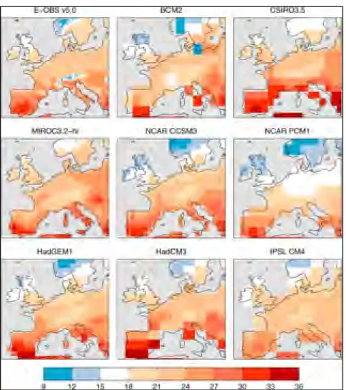
Figure 1.2 Mean summer maximum temperature for the reference period 1970–1999 from observations (E-OBS v5.0 0.5◦(Haylock
et al., 2008)) and a range of AOGCMs in the CMIP3 database. Taken from Hawkins et al. (2013, p. 20)
However, all of them have larger grid cells than the observed data in the upper left corner which clearly differs in intensity and distribution with the coarser datasets (Hawkins et al., 2013).
In the simulation of the water cycle, finer resolution is particularly necessary mainly because its variables are highly influenced by their spatial distribution (Music & Caya, 2009). Therefore, the demand for higher resolution in climate simulations has increased, so accurate and reliable climate impact and adaptation studies can be performed. Consequently,
downscaling procedures have become essential in order to provide an adequate resolution of climate simulations for hydrological studies at a regional scale (Chen et al., 2011; Prudhomme et al., 2002; Teutschbein & Seibert, 2010). The downscaling methods are the most used approaches in impact studies, mainly because with these techniques, it is possible to overcome differences in spatial and temporal scale between climate and hydrological models, and also to overcome biases present in climate model outputs (Riboust & Brissette, 2015).
Downscaling methods are mainly categorized as statistical or dynamic. Statistical downscaling produces future scenarios using statistical relationships between large-scale climate variables and regional characteristics identified from recent climate records. This process involves various techniques such as multiple regressions, stochastic generators and neural networks, which are used to establish the statistical relationships between observed local conditions and simulated climate variables (Diaz-Nieto & Wilby, 2005; Wilby et al., 1998). More recently, bias correction methods based on model output statistics have been used more and more frequently (Jakob Themeßl et al., 2011).
Figure 1.3 Regional climate model configuration Taken with the permission of Marco Braun (2017) Ouranos
Dynamic downscaling is based on climate models at fine resolution (from 10 km to 50 km) describing the atmospheric processes nested within GCM’s outputs. These are commonly named Limited Area Models (LAMs) or Regional Climate Models (RCMs) (R. Jones et al., 1995; Laprise, 2008). These models provide a more physically realistic representation of the regional climate at finer resolutions. RCMs, as shown in Figure 1.3, are provided with data from a driving model at the RCM boundaries of the domain to simulate. The driving model can be a GCM or another fine resolution gridded data product such as reanalysis datasets (Charron, 2014). Reanalysis data is high-resolution data which combines observations and climate simulations to produce recent past simulations that better represent the state of the atmosphere (Bengtsson & Shukla, 1988; Carter et al., 2007).
Consequently, large computational resources are required to perform these simulations. Nonetheless, the need for more accurate regional climate simulations has driven the creation of international initiatives such as the Coordinated Regional Downscaling Experiment (CORDEX) project (Giorgi & Gutowski, 2015). This programme creates a framework to generate an ensemble of regional-local scale climate projections for more adequate impact and adaptation studies (Giorgi et al., 2009). The CORDEX project assembles RCMs used around the world with a variety of domains, drivers and resolutions.
1.3.1 Climate projections: general trends
Due to the worldwide-observed climate change impacts, what will happen in the future is a fundamental issue for the modern society. Thus, climate models are used to simulate plausible scenarios and generate projections of the future (AghaKouchak et al., 2012).
Over the years, scientists have shown more confidence in the fact that the rising trend in the greenhouse gas concentrations will increase the global temperatures, yet there is lower confidence of how the climate will change at a regional scale (Giorgi et al., 2001). It is at the regional scale, such as that of a river catchment, that climate change will be noticed. Therefore, to generate predictions of climate change at these scales, it is necessary to use a
number of plausible future climates referred to as climate scenarios (Carter et al., 2007). The most recent generation of scenarios is the Representative Concentration Pathways (RCP), used for the ensemble of climate models in the CMIP5. Four RCPs were identified by the research community to address the new developments and thus allow climate models to represent the range of the latest climate policies (IPCC, 2013c; Moss et al., 2010). One mitigation scenario (RCP2.6), two stabilization scenarios (RCP4.5 and RCP6) and one scenario with very high greenhouse gas emissions (RCP8.5) are used to attempt to cover the largest range of plausible emissions (IPCC, 2013c). These four scenarios are represented by future radiative forcings (2.6, 4.5, 6 and 8.5), which describes the change on the atmosphere radiation balance (incoming and outgoing) caused by plausible changes in its constituents (Moss et al., 2010).
Climate scenarios are then used to produce climate projections, which attempt to represent the possible evolution of the different components within the climate system influenced by the different RCPs (Charron, 2014; Moss et al., 2010). However, it is important to note that climate scenarios are neither predictions nor forecasts. A climate scenario is only a plausible description of how the future could behave over long time scales , i.e. decades or centuries, according to stated assumptions regarding future trends in greenhouse gases emissions, changes in land use and population growth (IPCC, 2013c). For this reason, it is important to mention that the future remains uncertain, as the different scenarios are constructed on multiple assumptions that may or may not happen in the future.
The warming climate has affected the water cycle in different ways. The AR5 assembled observed evidence of these impacts. Observations with different measurement devices (i.e. stations, radiosondes, satellites, etc.) indicate increases of water vapour in the troposphere since the 1970s. Precipitation is harder to measure; however, decreasing snowfalls, increasing winter temperatures and significant seasonal reductions of snow cover have been observed (Stocker et al., 2013). Thus, along with these trends, future changes in the water cycle are expected to occur.
Projections of future changes suggest that increases in global precipitation and tropospheric water vapour are expected during the 21st century. However, in a much warmer world, these
changes are projected to be highly variable depending on the region and the season (IPCC, 2013b). Likewise, the global runoff projections remain highly uncertain due to the complexity of the interactions between different processes within the water cycle (Stocker et al., 2013).
1.3.2 Sources of uncertainty
Uncertainty has become one of the most important subjects in the studies of climate change. There are numerous sources of uncertainties in the process of hydrological modelling and climate change impact assessments (Prudhomme et al., 2003). This process has been studied during the last decade and is referred to as the “cascade of uncertainty” (Schneider, 1983; Wilby & Dessai, 2010) or the “uncertainty explosion” (Henderson-Sellers, 1993; R. N. Jones, 2000).
Different studies have identified sources of uncertainty and it has been agreed upon that the most important sources are the greenhouse emission scenarios, global climate model structure, downscaling method, impact (or catchment) model and the natural climate variability uncertainty (Falloon et al., 2014; Poulin et al., 2011; Wilby, 2005). Figure 1.4 shows the “cascade of uncertainty” which clearly illustrates the growth of the envelope of uncertainty from various sources starting with the uncertain future society to the accumulated uncertainty at the end to obtain adaptation responses.
The climate model is generally considered the most important source of uncertainty. Therefore, recent studies have analyzed other sources of uncertainty related to the GCM and RCM configurations. For example, P. Roy et al. (2014) showed that the largest source of uncertainty on simulation of precipitation extremes came from the model selection and domain size followed by the member selection during the summer months.
Figure 1.4 Cascade of uncertainty Taken from Wilby and Dessai (2010, p. 181)
It is seen that many sources of uncertainty can be included in the modelling chain. Therefore, the research community keeps working to identify and quantify the types of uncertainty that are the most important for each particular impact study (Hawkins et al., 2013).
1.4 Regional studies: Quebec
Water resources are of great importance in the province of Quebec, thus regional hydrological impact studies have been performed to analyse future projections of the hydrologic regime. Catchment-scale studies have been assessed in past and recent years in different regions of the province. Examples of such studies are presented by Minville et al. (2008), Minville et al. (2009),Chen et al. (2011), Arsenault et al. (2013), Troin et al. (2016) and Trudel et al. (2017) where RCMs outputs where used as inputs for climate change impact and uncertainty assessments.
More specifically, high flows have been investigated in different studies over the region. For example, L. Roy et al. (2001) assessed the impact of climate change on seasonal floods of the Châteauguay River Basin. Canadian GCM simulations coupled with a hydrological model were used to assess the floods for different return periods. The results indicated
potential augmentations of streamflow. Larger increases on this trend were showed when longer return periods were considered. Quilbé et al. (2008) evaluated the effects of climate change in the Chaudière River suggesting future increases on winter flows and decreases in spring flows as other authors have also implied (Boyer et al., 2010; L.-G. Fortin et al., 2007; Mareuil et al., 2007; Minville et al., 2008).
Local initiatives have emerged to provide an ample and homogeneous assessment of hydrological projections. The Hydroclimatic Atlas of Southern Quebec is a project involving various experts providing reliable hydrological projections over selected catchments in the province. The latest version of the Hydroclimatic Atlas of Southern Quebec (CEHQ, 2015) presented the following main trends expected on the water regimes for southern Quebec for the 2050 horizon (see table 1.1).
Table 1.1 Trends for the 2050 horizon for southern Quebec.
Taken from the Hydroclimatic Atlas of Southern Quebec (CEHQ, 2015, p. V)
Trends for the 2050 horizon Confidence
Spring high flow will come earlier High Spring high flow volume will be lower in southernmost Quebec Moderate The spring high flow peak will be lower in southernmost Quebec Moderate The summer and autumn high flow peak will be higher throughout large
areas of southern Quebec Moderate Summer low flow will be more severe and last longer High
Winter low flow will be less severe High Summer mean flow will be lower High Annual mean flow will be higher in the north of southern Quebec and lower
These trends were also confirmed in a larger study of hydrological projection over numerous catchments in the province (Guay et al., 2015). Higher winter flows and lower summer flows with earlier spring floods are expected. The height of snow cover along with the number of days with snow on the ground are likely to decrease in the south while more snow in a shorter season is expected in the north. However more research is still required as improved and finer climate datasets and approaches are constantly updated since they are expected to yield better representations of the climate system. Studies have analyzed the effects of the spatial resolution on the regional climate model outputs showing evidences of the gain, generally named “added value”, on the use of higher spatial resolutions on the Canadian RCM (Curry et al., 2016a; Lucas-Picher et al., 2016).
The spatial resolution increase also requires an increase in the climate model simulation times, which raises the need to evaluate how the spatial resolution in climate modelling impacts the hydrological streamflow simulations. In other words, it is necessary to analyse the effects of the higher climate model resolution on the simulation of hydrological extremes such as floods.
1.5 Research objectives
The main objective of this project is to analyse the impact of spatial resolution of different climate simulations issued from two different versions of the Canadian Regional Climate Model (CRCM) on the hydrological modelling of summer and fall floods in southern Quebec. In order to address the main objective, the following specific objectives will be investigated:
1. Evaluate the impact of increasing spatial resolution on temperature and precipitation climate model outputs.
2. Study the impact of the different hydrological models structure on summer and fall flood simulations.
3. Study the impact of hydrological model parameter set on summer and fall flood simulations.
CHAPTER 2
STUDY AREA AND DATA
2.1 Study area
This study was carried out over 50 watersheds located in southern and central Quebec (see Figure 2.1). This region covers a significant part of the integrated water resources management zones defined by the Ministère du Développement Durable, de l’Environnement et de la Lutte contre les Changements Climatiques (MDDELCC, 2017) and is part of the study area used in the latest Hydroclimatic Atlas of Southern Quebec (CEHQ, 2015).
Figure 2.1 Location and mean annual precipitation (mm) of the 50 watersheds used in this study
The Figure 2.1 shows the location of the selected watersheds along with their mean annual precipitation. The watersheds were selected in order to accomplish the following criteria:
1. Diversity of catchment area. In order to account for the effects in regions with different characteristics, the watersheds have a diversity of catchment areas ranging from 512 km2 to 18,983 km2.
2. Availability of data. Due to data availability, the meteorological and hydrometric observed data have a period length of at least 12 years to have representative datasets to perform the calibration and validation of the hydrological models. These datasets were obtained between 1969 and 2010 depending on the available hydrometric and meteorological records for each watershed.
3. Natural observed streamflow. The hydrometric data of all the watersheds is based on natural observed streamflows or weakly influenced but not restored (i.e. an estimate of the natural flow that is regulated by a reservoir). This condition is essentially needed to avoid any impact on the hydrological modelling due to streamflow regulations
2.2 Observed data
For this project, observed historical records of meteorological data (minimum temperature, maximum temperature and precipitation) and streamflow were used.
The meteorological data was obtained from the Centre d’Expertise Hydrique du Québec (CEHQ) unit from the MDDELCC. As described in the “Plateforme de modélisation hydrologique du Québec méridional” (CEHQ, 2014), the meteorological database is derived from the simple kriging interpolation of observations from 971 stations operated by the MDDELCC and 21 stations operated by Rio Tinto. The interpolated dataset forms a grid of 0.1° (≈ 11 km) resolution covering the domain limited from 43° to 55° latitude and 60° to -80° longitude with daily values for the 1969-2010 period.
The hydrometric data were obtained from the Banque de Données Hydriques (BDH) of the Centre d’Expertise Hydrique du Québec (CEHQ) covering the same period of the meteorological data on a daily time step for the 50 hydrometric stations.
2.3 Climate simulation data
The climate model simulations datasets used for this project were issued from the fourth and fifth versions of the CRCM and were provided by the Ouranos Consortium on Regional Climatology and Adaptation. The climate datasets issued from CRCM4 (version 4) cover the 1961-1990 period and the datasets issued from CRCM5 cover the 1981-2010 period. Four climate simulations issued from the CRCM4 and three issued from the CRCM5, with a variety of drivers, domains and resolutions were used (Table 2.1).
Table 2.1 Description of the CRCM climate datasets used in this study
Acronym* Version Driver Domain Resolution
15km (CGCM, CRCM4) QC 4.2.4 CGCM3.1v2 Quebec 15 km
45km (CGCM, CRCM4) AMNO 4.2.3 CGCM3.1v2 North America 45 km
15km (ERA40c, CRCM4) QC 4.2.4 ERA40C Quebec 15 km
45km (ERA40c, CRCM4) AMNO 4.2.3 ERA40C North America 45 km
12km (ERAint75, CRCM5) QC 5 v3331 ERA-Interim 75 Quebec 0.11° ≈ 12 km
24km (ERAint75, CRCM5) QC 5 v3331 ERA-Interim 75 Quebec 0.22° ≈ 24 km 48km (ERAint75, CRCM5) QC 5 v3331 ERA-Interim 75 Quebec 0.44° ≈ 48 km
2.3.1 Regional climate model (RCM)
In this work, two RCMs were used, the CRCM4 and the CRCM5. Even though they share continuous numbered versions, they are in fact two different climate models. The CRCM4 is a limited-area nested model developed at Université du Québec à Montréal (UQAM) based on the fully elastic nonhydrostatic Euler equations (Daniel Caya & Laprise, 1999; D. Caya et al., 1995; Music & Caya, 2007). The CRCM5 is based on a limited-area version of the Global Environment Multiscale (GEM) model used for Numerical Weather Prediction at Environment Canada and developed at the Centre pour l’Étude et la Simulation du Climat à l’Échelle Régionale (ESCER Centre) at the UQAM (Côté et al., 1998; Martynov et al., 2013). The CRCM5 provides a more realistic representation of water and energy exchange between the land surface and atmosphere and has contributed to the CORDEX project over North America (Lucas-Picher et al., 2016).
In order to attain the main objective, seven different climate datasets issued from the CRCM4 and the CRCM5 were evaluated. From CRCM4, four datasets were used. They consist of two datasets driven by the Canadian General Circulation Model (CGCM) third generation (Scinocca et al., 2008) and two driven by the ERA-40c reanalysis (Uppala et al., 2005). For each driver, the climate model was run at 45km and 15km resolution. As observed in Table 2.1, the four CRCM4 datasets also have different domains; the simulations at 45km resolution were simulated over North American domain, while the simulations at 15km .resolutions were simulated over Quebec domain. The maps of the different domains are presented in the appendix I
The three CRCM5 datasets share more similarities. All CRCM5 datasets were driven by the ERA Interim (Dee et al., 2011) reanalysis and were simulated over Quebec domain. The only difference between these three simulations by CRCM5 is their different spatial resolutions of 0.44° (≈ 48 km), 0.22° (≈ 24 km) and 0.11° (≈ 12 km) respectively.
CHAPTER 3 METHODS
3.1 Overview
The general methodology of the present project is described in the following schematic representation presented in Figure 3.1.
Figure 3.1 Overview of this project’s research methodology
The overall methodology is divided in three main parts, (1) the climate simulations comparison, (2) the hydrological modelling by two different hydrological models and (3) the summer-fall floods analysis by the use of 2, 5, 10 and 20-year return periods as flood indicators.
3.2 Climate data comparison
This study aims to analyse the effects of spatial resolution on summer-fall floods simulation. Thus, in order to address the main objective, the first specific objective is to evaluate the impact of increasing spatial resolution on temperature and precipitation datasets as simulated by the different versions of the CRCM.
The evaluation of the effects of spatial resolution on the climate datasets is done by comparing the differences between two simulations with different resolutions. Where a given simulation named “X” and another simulation named “Y” are compared and presented as X/Y, where Y is the simulation used as the reference dataset. A summary of the comparisons used to evaluate the spatial resolution impact is presented in Table 3.
Table 3.1 Summary of CRCM4 and CRCM5 climate datasets comparisons
Acronym* Version Driver Resolutions
15km (CGCM, CRCM4) QC / 45km (CGCM, CRCM4) AMNO 4.2.4 CGCM3.1v2 15 km / 45km 15km (ERA40c, CRCM4) QC / 45km (ERA40c, CRCM4) 4.2.4 ERA40C 15 km / 45km 12km (ERAint75, CRCM5) QC / 24km (ERAint75, CRCM5) QC 5 v3331 ERA-Interim 75 12 km / 24 km 12km (ERAint75, CRCM5) QC / 48km (ERAint75, CRCM5) QC 5 v3331 ERA-Interim 75 12 km / 48 km
*The acronym stands for: simulation X / simulation Y
Performance statistics were computed to evaluate the mean and variability differences between the compared CRCM4 and CRCM5 climate simulations. The comparisons of temperature and precipitation datasets were evaluated using the following metrics.
Mean seasonal temperature and precipitation
The climate datasets comparison was performed using the mean seasonal values for the temperature and precipitation datasets. The mean seasonal temperature ( ) and the mean seasonal precipitation ( ) were calculated as follows:
= ∑ ∑ (3.1)
= ∑ ∑
(3.2)
where and are the daily values of temperature or precipitation, is the number of days of the season and is the number of years of the full time series. The leap year day is removed from the datasets.
Temperature seasonal bias
The temperature seasonal bias is calculated between the mean seasonal temperatures of a given dataset x named and the mean seasonal temperatures of a reference dataset y named
as follows:
= − (3.3)
Precipitation seasonal relative bias
The precipitation seasonal relative bias is calculated between the mean seasonal precipitations of a given dataset x named and the mean seasonal precipitations of a reference dataset y named as follows:
Ratio of the seasonal variances
The variance ( ) describes the variability of the data in regards of the mean values of a determined dataset X (temperature or precipitation). The mean seasonal variance ( ) is calculated as follows:
= ∑ ∑ −
(3.5)
where is the daily value, is the mean value of the season for year i. These values are averaged by the number of years of the full time series. The leap year day is also removed from the datasets. The ratio of the seasonal variances (temperature or precipitation) is calculated between the mean variance of a given dataset x named and the mean variance of a reference dataset y named as follows:
ℎ = (3.6)
These metrics were selected to quantify the differences between the climate simulations with different spatial resolutions to evaluate their impacts. Thus, no comparisons were made with actual historical observations.
3.3 Hydrological modelling
The hydrological modelling was performed by two lumped conceptual models with different structures and levels of complexity in order to study the impact of the hydrological model structure. These models have been largely used in research on the province of Quebec and were selected due to their availability and relatively short time of simulation.
3.3.1 Hydrological models
HSAMI model
The HSAMI hydrological model (V. Fortin, 2000), has been used by Hydro-Quebec over the province of Quebec during the last decades and has been applied in numerous studies (e.g. Arsenault et al., 2013; Chen et al., 2011; Minville et al., 2008; Poulin et al., 2011). HSAMI is a lumped conceptual model based on reservoirs that simulates the main processes of the hydrological cycle. To perform a simulation, the inputs required are the mean values of maximum and minimum temperatures over the selected area, precipitation (liquid and solid) and cloud cover fraction. The model has up to 23 calibration parameters, all of which were calibrated by the Covariance Matrix Adaptation Evolution Strategy (CMAES) (N. Hansen & Ostermeier, 1997) as recommended by Arsenault et al. (2014).
MOHYSE model
The MOHYSE model is a simpler lumped conceptual model that was developed byV. Fortin and Turcotte (2006). The model has been used in different studies in Canadian watersheds such as the studies presented by Arsenault (2015) and Velázquez et al. (2010). MOHYSE simulates the main hydrological processes and can be run on different time scales (from sub-daily to multiple days). The required input data are mean sub-daily temperatures, total sub-daily rain and snow. All of these values are averaged over the watershed since the model is lumped. This model has ten parameters, all of which were also calibrated with the CMAES algorithm.
3.3.2 Calibration and validation
The calibration of the hydrological models was performed on the odd years of the 1969-2010 period using three different objective functions since quantifying the impact of hydrological model parameter set is one of the specific aims of the project. The three objective functions are variations of the Kling-Gupta Efficiency criterion previously described in the equations 1.1 to 1.4.
The first objective function used for this project is the KGE over the calibration period. The second objective function is the KGE value over the summer-fall months (June to October) to give focus to those seasons which are of interest in this study. Finally, the third objective function consists of a custom criterion combining the KGE value of the interannual mean hydrograph and the KGE on the summer-fall months to focus on the summer-fall period and also to avoid sacrificing the rest of the hydrograph. Table 3 presents a summary of the three objective functions.
Table 3.2 Summary of the objective functions for the hydrological model’s calibration
Acronym Description OF-1
OF-2 OF-3
2 + 2
This KGE criterion measures the goodness of fit between two datasets (observed and simulated streamflow in this case) ranging from –Infinite to 1, where a value of 1 indicates a perfect fit between the datasets, a value of 0 means a good fit on average values and negative values indicates worse fitting than using the mean as a predictor. The validation was then performed on the even years (not calibrated) for each watershed.
3.3.3 Streamflow simulations
After analyzing the CRCM climate outputs, the hydrological modelling was performed to evaluate the impacts of the climate simulations spatial resolution on the floods modelling. To address this issue, streamflow simulations driven by the seven CRCM climate datasets (temperature and precipitation) were generated and compared.
To generate the streamflow simulations, the hydrological models were firstly calibrated and validated with historical records of observed streamflows in order to evaluate their performance in summer-fall floods estimations for the three different objective functions. Thus, three different parameter sets were obtained for both hydrological models on each of the fifty watersheds. In this way, along with the main objective, the impacts of hydrological model structure (specific objective 2) and the impacts of model parameter set (specific objective 3) are also investigated by comparing the results of the hydrological models and the different calibration approaches.
Once the hydrological models are validated, the CRCM climate datasets are directly used as input for the hydrological models to produce the climate driven streamflow simulations. It is important to mention that no recalibration was performed to generate the climate driven streamflow simulations. This approach was fixed in order to avoid any influence on the extreme events magnitude and frequency due to the recalibrations, as they are expected to have a diminishing effect on the data’s variability, a characteristic important to preserve in the analysis of extreme events such as floods. Thus, the parameter sets obtained in the calibration process were preserved to produce the different streamflow simulations to later be inter-compared. Therefore, seven (7) climate driven streamflows for both hydrological models (2) each calibrated on three (3) objective functions and fifty (50) watersheds were then generated.
The climate-driven streamflow simulation comparison was done following the same approach described for the climate datasets comparison. The comparisons were performed between two different climate driven streamflow simulations (as performed in the climate data comparison), where a given streamflow simulation “X” and another streamflow simulation “Y” are compared, using Y as the reference dataset (presented as X/Y). The climate driven streamflow simulations comparisons were made by using two performance statistics to measure the difference between two datasets: The seasonal KGE value described previously in the equations 1.1 to 1.4 and the seasonal relative bias (%) described in the equation 1.7.
3.3.3.1 Return Periods
The main objective of the study is to identify the effects of the spatial resolution on flood events. Thus, four flood indicators were defined to evaluate the spatial resolution impact: the 2-year, 5-year, 10-year and 20-year return period of summer-fall floods. The different climate datasets have a length of 30 years, thus, the four flood indicators were defined in function of the sample size. In this manner, the datasets have a valid sample size (30 values of annual summer-fall peak flows) to estimate representative distributions for each flood indicator. The four return periods were estimated from the simulated climate driven streamflows by a flood frequency analysis using the Gumbel distribution. This distribution is often used in hydrology to represent flood peaks distributions due to its commonly good approximations and simplicity of use (Chebana & Ouarda, 2011; Loaiciga & Leipnik, 1999; Marques et al., 2015; Yue et al., 1999).
The return periods are compared using the same approach that was described for the climate simulations and the streamflow simulations, where a given flood indicator “X” and another flood indicator “Y” are compared and presented as X/Y. The comparisons between the estimated return periods were done by using the relative bias (%) as an evaluation metric:
%) = − ∙ 100% (3.6)
where Y is the value used as a reference.
This metric was used to quantitatively evaluate the impact of the spatial resolution in the different estimated flood indicators estimated from the generated climate-driven summer-fall peak flows.
CHAPTER 4 RESULTS
The results are presented in three main sections. First, the comparisons between the climate simulations with different resolutions (temperature and precipitation) are presented. Second, the hydrological modelling performance is shown for calibration and validation years in regards of observed data over the fifty watersheds. Finally, the climate driven streamflow simulations are compared and analyzed by calculating the different performance statistics over the streamflow simulations and the flood indicators.
4.1 Climate simulations intercomparison
As presented in chapter 3, the first stage of the methodology consists in the analysis of the CRCM climate simulations. To that effect, four comparisons were done to evaluate the impact of spatial resolution over the province of Quebec: two comparisons for the climate outputs issued from the fourth version of the CRCM and two comparisons between simulations issued from the fifth version of the CRCM.
4.1.1 Spatial resolution
4.1.1.1 Temperature
Figures 4.1 and 4.2 present maps of the annual daily mean temperature (°C) bias between simulations with different resolutions issued from CRCM4 and CRCM5, respectively. Each figure shows the bias between two temperature simulations with different resolutions. No comparisons were done against observations. The maps show the bias for the summer (June, July and August) and fall (September, October and November) seasons over the province. The fifty watersheds of the study area are highlighted in black.
Figure 4.1 Annual daily mean temperature (°C) bias between simulations issued from CRCM4 for the summer (JJA) and fall (SON) seasons for the period 1961-1990.The upper
panels (a) show the comparisons for the datasets driven by CGCM. The lower panels (b) show the comparisons for the datasets driven by ERA40c
On the comparisons of temperature datasets issued from CRCM4 driven by CGCM (upper panel on Figure 4.1) a consistent hot bias is observed during the fall months. More variability is observed during the summer months with a bias varying between 2 and -2 degrees Celsius. On the other hand, the comparisons of the ERA40c-driven simulations show similar trends on the summer and fall seasons. A general cold bias is observed over the province with some hot spots on the center and southern regions of the province. This is true for both seasons with a slightly hotter bias observed during the summer months.
a)
For the comparisons of temperature datasets issued from CRCM5 (see Figure 4.2), two comparisons are presented. The bias between the 12 km and 24 km resolution (top two panels) shows a consistent cold bias over the entire region during the fall months. Smaller and generally cold biases are observed during the summer with some hot biases observed close to the coastal areas. Similar trends are also observed for the 12 km and 48 km resolutions comparison (bottom two panels), yet, the range of bias is slightly larger, reaching values of up to 3 degrees Celsius difference.
Figure 4.2 Annual daily mean bias of temperature (°C) between simulations issued from CRCM5 for the summer (JJA) and fall (SON) seasons for the period 1981-2010.The upper panels (a) show the comparisons for the datasets with 12 km and 24 km resolution. The lower
panels (b) show the comparisons for the datasets with 12 km and 48 km resolution
a)
It can be observed in Figure 4.3 that the 15 km resolution datasets have larger variances than the 45 km resolution datasets in the northern parts of the province for both seasons and both drivers. Mean differences of 15 % are observed for the CGCM-driven comparison while differences of up to 50 % are shown for the ERA40c- driven comparisons. In the south (over the study region), the 15 km resolution presents smaller variances (around 5 to 15 % difference) than the 45 km resolution temperature variances. The CGCM-driven comparison shows larger differences during the fall and the ERA40c-driven comparison shows larger variance difference during the summer.
Figure 4.3 Ratio of annual seasonal mean temperature variances between simulations issued from CRCM4 for the summer (JJA) and fall (SON) seasons for the period 1961-1990.The upper panels (a) show the comparisons for the datasets driven by CGCM. The lower panels
(b) show the comparisons for the datasets driven by ERA40c
a)