Pearl River basin in Southern China
Author(s)
Niu, J; Chen, J; Bellie, S
Citation
Hydrology and Earth System Sciences, 2014, v. 18 n. 4, p. 1475-
1492
Issued Date
2014
URL
http://hdl.handle.net/10722/197592
www.hydrol-earth-syst-sci.net/18/1475/2014/ doi:10.5194/hess-18-1475-2014
© Author(s) 2014. CC Attribution 3.0 License.
Hydrology and
Earth System
Sciences
Teleconnection analysis of runoff and soil moisture over the
Pearl River basin in southern China
J. Niu1, J. Chen1, and B. Sivakumar2,3
1Department of Civil Engineering, The University of Hong Kong, Pokfulam, Hong Kong, China
2School of Civil and Environmental Engineering, The University of New South Wales, Sydney, NSW 2052, Australia 3Department of Land, Air and Water Resources, University of California, Davis, CA 95616, USA
Correspondence to: J. Chen ([email protected])
Received: 26 July 2013 – Published in Hydrol. Earth Syst. Sci. Discuss.: 30 September 2013 Revised: 6 February 2014 – Accepted: 7 March 2014 – Published: 23 April 2014
Abstract. This study explores the teleconnection of two
cli-matic patterns, namely the El Niño–Southern Oscillation (ENSO) and the Indian Ocean Dipole (IOD), with hydrolog-ical processes over the Pearl River basin in southern China, particularly on a sub-basin-scale basis. The Variable Infil-tration Capacity (VIC) model is used to simulate the daily hydrological processes over the basin for the study period 1952–2000, and then, using the simulation results, the time series of the monthly runoff and soil moisture anomalies for its ten sub-basins are aggregated. Wavelet analysis is per-formed to explore the variability properties of these time se-ries at 49 timescales ranging from 2 months to 9 yr. Use of the wavelet coherence and rank correlation method reveals that the dominant variabilities of the time series of runoff and soil moisture are basically correlated with IOD. The in-fluences of ENSO on the terrestrial hydrological processes are mainly found in the eastern sub-basins. The teleconnec-tions between climatic patterns and hydrological variability also serve as a reference for inferences on the occurrence of extreme hydrological events (e.g., floods and droughts).
1 Introduction
Regional responses of hydrological processes to climate vari-ability are often different from one river basin to another (Eltahir, 1996). Accordingly, the different sub-basins of a large-scale river basin may play their own roles in modu-lating the influences of climatic patterns (Chen and Kumar, 2002, 2004; Markovi´c and Koch, 2005) and in manifesting the tendency of flood or drought occurrence due to extreme
precipitation. Therefore, an important step in the assessment and prediction of floods or droughts is to understand the re-lationships between the key hydrological variables (e.g., pre-cipitation, runoff, soil moisture) and climate patterns.
Generally speaking, observations of hydrological vari-ables over large-scale basins are scarce, except for precip-itation. For instance, even though streamflow gauging sta-tions currently exist along most large rivers around the world, long-term flow observations are still not available, especially for sparsely populated regions and complex terrains. In ad-dition, while soil moisture is a key component of the hydro-logical cycle, it is also one of the least observed hydrologi-cal variables in terms of spatial and temporal coverage. Be-cause of the lack of long-term and large-scale observations of runoff and soil moisture, utilization of hydrological vari-ables forced by observed precipitation and other near-surface meteorological data is considered as a sensible and viable alternative in hydrological and water resources studies. For instance, using a macroscale hydrological model, the Vari-able Infiltration Capacity (VIC) model, Niu and Chen (2009, 2010) simulated the daily terrestrial hydrological processes over the Pearl River basin in southern China, and routed the simulated runoff to the downstream control stations of three major tributaries (i.e., the West River, the North River, and the East River).
In the specific context of the Pearl River basin, many other recent studies have also helped advance our understanding of the hydrological variability over the basin and the sur-rounding regions, including those on precipitation (e.g., Cui et al., 2007; Yang et al., 2010; Fischer et al., 2012; Chen et al., 2011; Zhang et al., 2012) and runoff (S. R. Zhang et al.,
2008; Niu and Chen, 2010), among others. For instance, sev-eral studies have reported that the significant fluctuations in precipitation over the basin are associated with atmospheric circulation patterns (Li and Zhou, 2012; Niu, 2013) influenc-ing the monsoon system over the region (Zhang et al., 2010; Zhou et al., 2012). Zhang et al. (2013) examined the me-teorological drought tendencies based on the standardized precipitation index by employing copula functions and the Mann–Kendall trend test. The Pearl River basin was cate-gorized into six regions based on latitude, longitude, eleva-tion, and the mean annual precipitation using the L-moments approach (Yang et al., 2010), and four homogenous regions based on the changing properties of precipitation using the kmean clustering algorithm (Zhang et al., 2012). Zhang et al. (2009) analyzed the scaling and persistence features of the long, daily streamflow series for four hydrological sta-tions on the mainstream of the East River. The changes of observed water discharge and sediment load (1950s–2004) were analyzed by S. R. Zhang et al. (2008) for nine stations in the Pearl River basin, although performed only on annual timescale. Despite these developments, it must be recognized that these studies were mainly performed based on observed data, the exceptions being those of Niu and Chen (2009, 2010).
Following up on the studies by Niu and Chen (2009, 2010), the present study evaluates the sub-basin hydrologi-cal processes over the Pearl River basin in response to two large-scale climatic patterns, the El Niño–Southern Oscilla-tion (ENSO) and the Indian Ocean Dipole (IOD), in order to improve our understanding of basin-featured flood and drought occurrences. Compared with the previous studies over the Pearl River basin, our focus in this study is on runoff and soil moisture processes, particularly on a sub-basin scale basis. Although runoff and soil moisture processes are gen-erally driven by precipitation, details of the analysis of pre-cipitation on sub-basin scale over the basin are not presented here. For such details, the interested reader is directed to the studies by Niu (2013), which present extensive investigations on the precipitation process over the basin as well as its tele-connections with climatic patterns.
In this study, we attempt to address the following spe-cific question: are there some characteristic periods and vari-ability processes of different hydrological variables within the Pearl River basin that may be related to climatic pat-terns, which may be a possible trigger for major floods or droughts (i.e., extreme hydrological events) in the basin? We address this question through (1) investigation of the possible variability linkages between the runoff/soil mois-ture and the above two climatic patterns, and (2) discus-sion of the underlying causes for extreme hydrological events from this perspective. For analysis, we consider data over the period 1952–2000, similar to the period studied by Niu and Chen (2009, 2010). To identify the patterns and capture the differences in continuous timescales of fluctuation em-bedded in the hydrological time series (i.e., streamflow and
soil moisture), we employ wavelets, in particular continuous wavelet transform.
Torrence and Compo (1998) developed a significance test for the wavelet power spectrum to provide quantita-tive results and reliable insights, and make the applications of continuous wavelet transform extensive. Subsequently, Grinsted et al. (2004) discussed the cross-wavelet trans-form and wavelet coherence for the applications to geo-physical time series in examining relationships between time series in a time–frequency domain. Meanwhile, Maraun and Kurths (2004) suggested that the interpretation of non-normalized cross spectra for the interrelation between two processes is not straightforward if not including appropriate confidence intervals, as it may show misleading peaks when just one of the time series has a strong peak. Further, Schaefli et al. (2007) reviewed recent developments in wavelet spec-tral analysis, recommended the calculation of wavelet coher-ence in the applications, and provided a valuable example to illustrate the usefulness of wavelet spectral analysis for detecting the flood-triggering situations in the Alpine catch-ment. In addition, the importance of the pervious knowledge about the physical processes and a methodologically rigorous significance testing are presented for the proper application and interpretation of the wavelet spectral analysis (Maraun and Kurths, 2004; Schaefli et al., 2007; Maraun et al., 2007). The rest of this paper is organized as follows. Section 2 gives details of the Pearl River basin study area and data considered for analysis. Section 3 describes the methods, in-cluding Morlet wavelet transform, the wavelet coherence and Spearman’s rank correlation. Section 4 presents the results and discussions from the wavelet application to runoff and soil moisture data in the study basin. Section 5 discusses the underlying causes of major flood/drought events in the basin. Conclusions are drawn in Sect. 6.
2 Background
2.1 The Pearl River basin
The Pearl River basin in southern China has a total area of about 450 000 km2, and consists of four main components: the East River, the North River, the West River and the Pearl River delta. The basin is located in a tropical and subtrop-ical monsoon climate region (Pearl River Water Resources Commission, 2005), with a long-term average annual pre-cipitation of about 1480 mm yr−1and mean annual
temper-ature ranging from 14 (in the western part) to 22◦C (in the
eastern part). As the largest river in terms of the rate of an-nual runoff generation (about 740 000 m3km−2yr−1) among the seven major rivers in China (i.e., the Yangtze River, the Yellow River, the Songhua River, the Pearl River, the Huai River, the Hai River, and the Liao River), the Pearl River ex-periences an abundant amount of variability in the terrestrial hydrological processes. For instance, the runoff ratio of the
Fig. 1. The Pearl River basin in South China, gauge stations, and 10 sub-basins (after Niu, 2013).
Fig. 1. The Pearl River basin in southern China, gauge stations, and 10 sub-basins (after Niu, 2013).
wettest year to the driest year is as high as 6–7, and about 80 % of the total annual runoff occurs in the wet season of April–September (Niu and Chen, 2009). As a consequence, extreme hydrological events frequently occur over the basin (Pearl River Hydraulic Research Institute, 2007; Cui et al., 2007). For example, a basin-scale flood occurred in 1994 and a severe drought event in 1963.
With due consideration to hydrological factors, water resources management, topographic features, and climate zones, this study divides the basin into ten sub-basins for analysis, similar to the approach by Niu (2013). These sub-basins are the East River, the North River, and the eight sub-basins in the West River basin (i.e., the Guihe, Lijiang, Hongshui, Beipan, Nanpan, Youjiang, Zuoyu, and the West River’s lower reach) (see Fig. 1). The sub-basin areas range from 29 000 to 58 600 km2, and the mean annual
precipita-tion varies from 1072 to 1772 mm yr−1. 2.2 Model simulation
2.2.1 Hydrological model
To obtain runoff and soil moisture data over the Pearl River basin, we adopt the VIC hydrological model to simulate such data. The VIC model (Liang et al., 1994) is a macroscale hydrological model, usually applied with spatial resolutions ranging from 0.125 to 2◦latitude/longitude and from hourly to daily temporal resolutions (Nijssen et al., 2001a, b; Maurer et al., 2002; Sheffield et al., 2004; Troy et al., 2008). The model uses the variable infiltration curve (Zhao et al., 1980), which allows for the representation of subgrid variability in
soil storage capacity and infiltration capacity, and the param-eterization of baseflow as a nonlinear recession curve from the bottom soil layer (Dümenil and Todini, 1992; Todini, 1996). The land surface of the study area is represented by a specified number of tiled land cover classes (e.g., cropland, grassland) and the soil column is divided into three soil lay-ers. The total runoff of each grid cell is the sum of the over-land runoff and baseflow obtained for each grid cell (Nijssen et al., 1997).
2.2.2 Forcing and output data
The terrestrial hydrological processes over the Pearl River basin are simulated by the VIC model for the period 1952– 2000, with 1◦×1◦spatial resolution at daily time steps (Niu and Chen, 2010). The GTOPO30 DEM (digital elevation model) data set with 1 km spatial resolution (Verdin and Verdin, 1999) is used to delineate the Pearl River basin. Meteorological forcings, including daily precipitation, max-imum and minmax-imum temperature, wind speed, and relative humidity, reported in Feng et al. (2004), are used. The veg-etation and soil data are extracted from two global data sets provided by Nijssen et al. (2001a). The vegetation data are derived from the 1 km vegetation database of the Univer-sity of Maryland, on the basis of Advanced Very High Res-olution Radiometer (AVHRR) data (Hansen et al., 2000). The soil texture and soil bulk density are derived from the 5 min FAO-UNESCO (Food and Agriculture-United Nations Educational, Scientific, and Cultural Organization) digital soil map of the world and the WISE (World Inventory of Soil Emission Potentials) Pedon database; the remaining soil
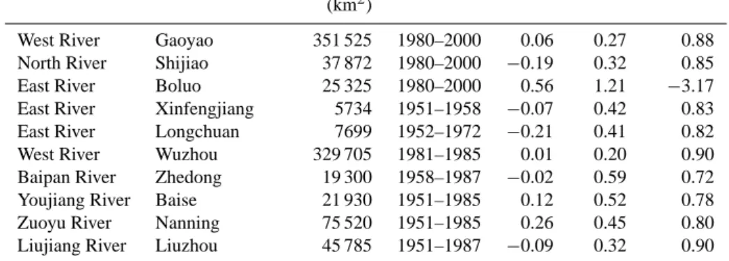
Table 1. Runoff simulation results at a monthly time step for 10 gauging stations over the Pearl River basin (in Fig. 1).
River Station Control area Period RB RRMSE NSE
(km2)
West River Gaoyao 351 525 1980–2000 0.06 0.27 0.88
North River Shijiao 37 872 1980–2000 −0.19 0.32 0.85
East River Boluo 25 325 1980–2000 0.56 1.21 −3.17
East River Xinfengjiang 5734 1951–1958 −0.07 0.42 0.83
East River Longchuan 7699 1952–1972 −0.21 0.41 0.82
West River Wuzhou 329 705 1981–1985 0.01 0.20 0.90
Baipan River Zhedong 19 300 1958–1987 −0.02 0.59 0.72
Youjiang River Baise 21 930 1951–1985 0.12 0.52 0.78
Zuoyu River Nanning 75 520 1951–1985 0.26 0.45 0.80
Liujiang River Liuzhou 45 785 1951–1987 −0.09 0.32 0.90
parameters are obtained based on the study of Cosby et al. (1984). The thicknesses of the three soil layers over the Pearl River basin are 0.3 m (the upper layer), 1.0–2.5 m (the second layer), and 0.2 m (the bottom layer), respectively.
The VIC-model’s daily simulation results are compared with the observations at a monthly scale after aggregation of daily data. The available streamflow observations at 10 gaug-ing stations (i.e., Gaoyao, Shijiao, Boluo, Zhedong, Baise, Nanning, Liuzhou, Wuzhou, Xinfengjiang, and Longchuan) in the basin (see Fig. 1) are used (Niu and Chen, 2010). The monthly scale is chosen for (1) the more “acceptable” accu-racy of the model simulation results, and (2) the compatibil-ity with the large-scale climate indices data. Table 1 presents a comparison between the observations and the model simu-lations of streamflow data for these 10 stations, by employ-ing three objective functions (i.e., relative bias – RB, relative root mean square error – RRMSE, and Nash–Sutcliffe effi-ciency – NSE – coefficient). The comparison suggests that the VIC model can simulate reasonably well the streamflow from the North River and the West River with its several sub-basins. However, there is a considerable discrepancy be-tween the streamflow simulations and the observations for the Boluo station in the East River. The studies by Niu and Chen (2010) and Wu and Chen (2012) have revealed that the Boluo streamflow is heavily regulated by the reservoirs in the upstream of the station. Therefore, the observations without the reservoir influences from two upstream stations (Xinfengjiang and Longchuan) are also used herein to eval-uate the streamflow simulations in the East River basin. The new results for the East River basin are comparable to the re-sults for the other stations in the North or West River basins (see Table 1). Based on the performance ratings suggested by Moriasi et al. (2007), the streamflow simulations at a monthly time step in the Pearl River basin in this study are evaluated as “satisfactory” (NSE>0.5 and RB<±0.25). With the val-idation of the VIC model performance, the monthly time se-ries of runoff and soil moisture are further aggregated for the 10 sub-basins (see Fig. 1 for their locations), and the wavelet-based analysis is carried out for the monthly runoff and soil
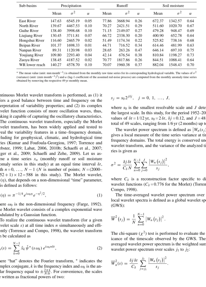
moisture anomalies for the sub-basins for the study period 1952–2000. It is also noted that the routing effects are ef-fective within 2–3 weeks for the Pearl River basin (Niu and Chen, 2010), and thus the monthly scale we choose, as the basis of the teleconnection study, is larger than the effective timescale of the routing effects. Table 2 lists the basic statis-tical properties for the observed precipitation and simulated runoff and soil moisture over the 10 sub-basins in the basin.
2.2.3 Large-scale climatic patterns
Two prominent large-scale climatic patterns influencing southern China (Saji et al., 1999; Guan and Yamagata, 2003; Zhou and Chen, 2007; Zhang et al., 2007), ENSO and IOD, are selected for examining the influence of large-scale climatic patterns on the hydrological processes in the Pearl River basin. The ENSO indices used are obtained from the monthly data of the National Oceanic and Atmo-spheric Administration (NOAA) Niño 3.4 (5◦N–5◦S, 170– 120◦W) SST (sea surface temperature; Trenberth and Stepa-niak, 2001; Labat, 2010a) for the base climatological pe-riod 1952–2000. The intensity of the IOD is characterized by an anomalous SST gradient between the western equatorial Indian Ocean (10◦S–10◦N, 50–70◦E) and the southeastern equatorial Indian Ocean (10◦S–0◦N, 90–110◦E). The IOD indices used are the combination of monthly IOD indices (1952–1997) from the Hadley Centre Global Sea Ice and Sea Surface Temperature (HadISST) data set and monthly IOD indices (1997–2000) from the NOAA Optimum Interpolation (OI) SST data set (Saji et al., 1999).
3 Methods
3.1 Morlet wavelet transform
As the continuous wavelet transform is suitable for analyz-ing nonstationary signals (such as streamflow and soil mois-ture) and identifying the temporal localization of dominant events, such wavelets are considered here. In particular, the
Table 2. Statistical properties of the observed precipitation and the simulated monthly time series (1952–2000) of 10 sub-basins over the
Pearl River basin.∗
Sub-basins Precipitation Runoff Soil moisture
Mean σ2 α Mean σ2 α Mean σ2 α
East River 147.63 6545.19 0.05 77.86 3668.94 0.26 672.37 1342.57 0.64 North River 139.67 4467.53 0.10 70.27 2421.51 0.29 511.60 1020.70 0.67 Guihe River 138.40 3998.68 0.10 71.15 2149.07 0.27 479.28 948.47 0.69 Liujiang River 130.45 3711.81 0.07 66.72 2338.30 0.20 400.90 652.78 0.64 Hongshui River 116.60 2465.79 0.02 51.49 1174.34 0.22 525.82 738.16 0.68 Beipan River 101.37 1698.33 0.01 44.71 716.52 0.34 614.46 481.99 0.63 Nanpan River 89.31 1120.98 0.03 28.65 263.26 0.47 646.14 697.10 0.75 Youjiang River 109.80 2293.40 0.04 42.14 676.54 0.38 810.84 1198.27 0.73 Zuoyu River 138.45 4187.52 0.02 70.77 1817.86 0.26 844.51 1088.41 0.64 WR lower reach 140.27 4578.70 0.10 70.07 1960.38 0.37 882.04 1548.43 0.70
∗The mean value (unit: mm month−1) is obtained from the monthly raw time series for its corresponding hydrological variable. The values ofσ2
(variance) (unit: (mm month−1)2) andα(lag-1 coefficient of the assumed red-noise process) are computed from the monthly anomaly time series obtained by removing the respective 49 yr monthly mean.
continuous Morlet wavelet transform is performed, as (1) it offers a good balance between time and frequency on the interpretation of variability properties; and (2) its complex wavelet function consists of more oscillation waves, thus, making it capable of capturing the oscillatory characteristics. The continuous wavelet transform, especially the Morlet wavelet transform, has been widely applied and tested to reveal the variability features in a time–frequency domain, including for geophysical, climatic, and hydrological time series (Kumar and Foufoula-Georgiou, 1997; Torrence and Webster, 1999; Labat, 2006, 2010b; Schaefli et al., 2007; Özger et al., 2009; Schaefli and Zehe, 2009). Let us as-sume a time series xn (monthly runoff or soil moisture anomaly series in this study) at an equal time interval δt, withn= 0, . . . , N−1 (N is number of points; N= (2000– 1952+1)×12 = 588 in this study). The Morlet wavelet, ψ0(η), that depends on a non-dimensional “time” parameter,
η, is defined as follows: ψ0(η)=π−1/4eiω0ηe−η
2/2
, (1)
whereω0 is the non-dimensional frequency (Farge, 1992).
The Morlet wavelet consists of a complex exponential wave modulated by a Gaussian function.
To realize the continuous wavelet transform (for a given wavelet scales) at all time indexnsimultaneously and effi-ciently (Torrence and Compo, 1998), the wavelet transform can be calculated as Wn(s)= N−1 X k=0 ˆ xkψˆ∗(s ωk) eiωknδt, (2)
where “hat” denotes the Fourier transform, ∗ indicates the complex conjugate,kis the frequency index andωkis the an-gular frequency equal to±2π k
N δt. For convenience, the scales are written as fractional powers of two:
sj =s02j δj, j =0,1, . . . , J, (3)
wheres0is the smallest resolvable scale and J determines
the largest scale. In this study, for the period 1952–2000, the values ofδt= 1/12 yr,s0= 2δt,δj= 0.12, andJ= 48 give a
total of 49 scales, ranging from 1/6 yr (2 months) up to 9 yr. The wavelet power spectrum is defined asWn(sj)
2
and gives a local measure of the time series variance at time and frequency domains. The total energy is conserved under the wavelet transform, and the variance of the analyzed time se-ries is given as σ2= δj δt CδN N−1 X n=0 J X j=0 Wn sj 2 sj , (4)
where Cδ is a reconstruction factor specific to different wavelet functions (Cδ= 0.776 for the Morlet) (Torrence and Compo, 1998).
The time-averaged wavelet power spectrum over all the local wavelet spectra is defined as a global wavelet spectrum (GWS): W2 sj= 1 N N−1 X n=0 Wn sj 2 . (5)
The chi-square (χ2) test is performed to evaluate the signif-icance of the timescale observed by the GWS. The scale-averaged wavelet power spectrum is the weighted sum of the wavelet power spectrum over scalesj1toj2:
W2n(s)= δj δt Cδ j2 X j=j1 Wn sj 2 sj . (6)
In addition, to display the variance evolution on the dominant variability band, the band-pass reconstruction is performed. The reconstructed time series is the sum of the real part of the wavelet transform (Torrence and Compo, 1998) over the above band: xn0 = δj δt 1/2 Cδψ0(0) j2 X j=j1 ReWn sj sj1/2 , (7)
where the factor ψ0(0) removes the energy scaling,
ReWn(sj) is the real part of the transform, ands1j/2 con-verts the wavelet transform to an energy density.
3.2 Wavelet coherence
The wavelet coherence analysis is used to identify regions in a time–frequency domain where the two time series co-vary, but may not have a common high power (Grinsted et al., 2004). The software package on wavelet coherence by Grinsted et al. (2004) is employed here to provide both cor-relation analysis and rough information on the phase differ-ence between two time series in a time–frequency domain. For two given time series, xn and yn, with corresponding wavelet transforms WnX(s) andWnY(s), the cross spectrum is WnXY(s)=WnX(s) WnY∗(s). The wavelet coherence phase is defined as tan−1[imaginary part of
WnXY(s) / real part of
WnXY(s) ], and the wavelet coherence of two time series is defined as Rn2(s)= S s−1WnXY(s) 2 Ss−1 WnX(s) 2 ·Ss−1 WnY(s) 2, (8)
whereSis a smoothing operator, defined as (Grinsted et al., 2004):
S(W )=Sscale(Stime(Wn(s))) , (9) whereSscale is the smoothing along the wavelet-scale axis
and Stime is the smoothing in time. A suitable smoothing
operator for the Morlet wavelet is given by Torrence and Webster (1999) as follows: Stime(W )|s = Wn(s)·c −t2 2s2 1 ! |s , (10) Sscale(W )|n = Wn(s)·c2 Y (0.6s) |n, (11)
wherec1 andc2 are normalization constants, andQ is the
rectangle function. The value 0.6 represents the decorrela-tion length of the empirically determined scale for the Morlet wavelet. The statistical significance level of the wavelet co-herence is estimated based on a large ensemble of surrogate data set pairs with the same lag-1 autoregressive (AR1) co-efficients given by Grinsted et al. (2004). The global wavelet coherence spectrum can be obtained by averaging the local wavelet coherence spectrum in time, and is helpful to ex-amine the characteristic scales (Torrence and Compo, 1998; Labat, 2010a).
3.3 Rank correlation
The Spearman’s rank correlation coefficientrS is applied to
measure the association between the ranks of two time series of scale-averaged wavelet power (xnandyn). The rank corre-lation analysis is used here because the transformed wavelet-power time series, for either an individual timescale or a timescale band, normally does not follow Gaussian distribu-tion (Torrence and Webster, 1999). The scored is calculated after ranking bothxnandyn, which is the difference between the rank onxnand the rank onyn.
rS =1− 6P d2 n n2−1 ! (12)
The significance test of the Spearman’s correlation hast and zversions as
to =rS
s
n−2
1−rS2, (13)
where significance statistictohas (n−2) degrees of freedom, and
zo=rS
√
n−1, (14)
where significance statistic zo has (n−1) degrees of free-dom. Following the now-familiar rules (Asquith, 2008), the t test is used when the cases or paired data points are fewer than 30, whilezis used for 30 cases or more.
4 Results and discussion 4.1 Wavelet power spectrum
In this study, ten sub-basins over the Pearl River are analyzed to examine the relationships between large-scale climatic patterns and local hydrological processes. Among these ten sub-basins, we consider the Boluo station in the East River for the purpose of illustration.
For the Boluo station, the monthly runoff anomaly time series is shown in Fig. 2a-i, and the normalized wavelet-power spectrum,|Wn(s)|2/σ2, is shown in Fig. 2a-ii; the hor-izontal axis is the time position over the period 1952–2000. In Fig. 2a-i, the anomaly data is obtained by removing the monthly mean for the period 1952–2000. In Fig. 2a-ii, the vertical axis has 49 timescales of the wavelet transform rang-ing from 2 months to 9 yr, and the strong variability power with greater than 95 % confidence is highlighted using white contours. We can observe that many abnormal runoff events (i.e., monthly runoff being too high or too low) appear at short timescales (e.g., less than 1 yr). Most of the wavelet power is distributed at the 1–4 yr band, and the strong vari-ability power, shown as white-contour enclosed regions, is found during the periods 1955–1970, 1980–1985 and 1990– 1995.
1955 1960 1965 1970 1975 1980 1985 1990 1995 2000 -200 -100 0 100 200 S oil m oist ur e (m m ) Time (year) P eri od ( year s) 1955 1960 1965 1970 1975 1980 1985 1990 1995 2000 0.25 0.5 1 2 4 8 0 2 4 6 8
Standardized wavelet power (b) 1955 1960 1965 1970 1975 1980 1985 1990 1995 2000 -200 0 200 400 Run off (m m ) Time (year) P er iod (y ea rs ) 1955 1960 1965 1970 1975 1980 1985 1990 1995 2000 0.25 0.5 1 2 4 8 0 2 4
Standardized wavelet power (a)
i.
ii. iii.
i.
ii. iii.
Fig. 2.
(a)
i.
Monthly runoff anomaly time series at Boluo station in the East River
and
ii.
Its local wavelet power spectrum using the Morlet wavelet, normalized by 1/
σ
2(
σ
2= 3,668.94 mm
2). The dashed curve depicts the cone of influence beyond which
the edge effects become important. The shaded contours are at normalized variances
of 1, 2 and 4. The white contour closes regions of greater than 95% confidence for a
red-noise process with a lag-1 coefficient
α
of 0.26.
iii.
Global wavelet power (solid
line with circles), mean red-noise spectrum (left dashed line), and 95% confidence
spectrum (right dashed line). (b) same as (a) but for soil moisture, in which (
σ
2=
1,342.57 mm
2,
α
= 0.64).
Fig. 2. (a) (i) Monthly runoff anomaly time series at Boluo station in the East River and (ii) its local wavelet power spectrum using the Morlet
wavelet, normalized by 1/σ2(σ2= 3668.94 mm2). The dashed curve depicts the cone of influence beyond which the edge effects become important. The shaded contours are at normalized variances of 1, 2 and 4. The white contour closes regions of greater than 95 % confidence for a red-noise process with a lag-1 coefficientαof 0.26. (iii) Global wavelet power (solid line with circles), mean red-noise spectrum (left dashed line), and 95 % confidence spectrum (right dashed line). (b) Same as (a) but for soil moisture, in whichσ2= 1342.57 mm2, and α= 0.64.
Figure 2a-iii shows the global wavelet power spectrum (GWS) of the monthly runoff anomaly data (see Eq. 5). As many geophysical time series can be modeled as red noise (Torrence and Compo, 1998), the figure also includes the mean and 95 % confidence level red-noise spectrum (left and right dashed lines) by using the lag-1 autocorrelation. It is observed that, over the 49 timescales, the highest runoff vari-ability is identified at the 1.92 yr scale, which is above the 95 % confidence level. This is consistent with the result ob-tained for precipitation data in the East River basin (Niu, 2013), where the highest precipitation variability is detected around the 2 yr band. The detected significant variability in-dicates less randomness of the underlying processes due to local influences, and it may well be related to external cli-matic patterns (see Sect. 4.4 for details).
Figure 2b shows the corresponding results for the monthly soil moisture in the East River basin. A comparison between
Fig. 2a-ii and b-ii reveals that the high variability power at short timescales for soil moisture almost disappears, while for larger timescales, the related power for soil moisture is enhanced. In the terrestrial hydrological processes, the river basin, like a buffer, reduces the high-frequency precipitation variability by runoff, and the long-term precipitation vari-ability is memorized by soil moisture. Figure 2b-iii shows that the variability power at short timescales is reduced much more, but improved at larger timescales (note that the magni-tude of the GWS is doubled compared to that in Fig. 2a-iii). Further, the detected highest variability is transferred from 1.92 (see Fig. 2a-iii) to 3.16 yr (see Fig. 2b-iii), with the large spikes (about 6 spikes) in Fig. 2a-ii appearing around the 2 yr scale, and the spikes with the largest area (in a time– frequency domain) exist around the 2 yr scale in Fig. 2b-ii.
4.2 Coherent modes of the GWSs
In addition to the analysis of the East River presented above, we further inspect their global variability distributions (i.e., GWSs) for the other nine sub-basins. Performing prin-cipal component analysis (PCA) on the GWSs over these 10 sub-basins, we find that there are three coherent modes for hydrological variabilities at the 49 timescales (see Fig. 3). The main steps in the PCA application in this study are as fol-lows: (1) a covariance matrix is obtained by using the wavelet power spectra for s (equal to 49) timescales of runoff/soil moisture in 10 sub-basins; (2) the covariance matrix is de-composed to get eigenvectors of the matrix, which accounts for the maximum amount of the joint variability of anomalies of initial wavelet power spectrum at each sub-basin; (3) the new variables are produced after projecting the data on the obtained eigenvectors; (4) the first three principal compo-nents are selected for runoff and soil moisture, respectively; and (5) each sub-basin is then classified as belonging to the mode where its coefficient of the eigenvectors (i.e., the length of the vector projected on corresponding direction) is the largest absolute value.
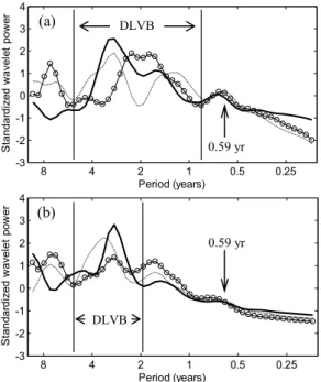
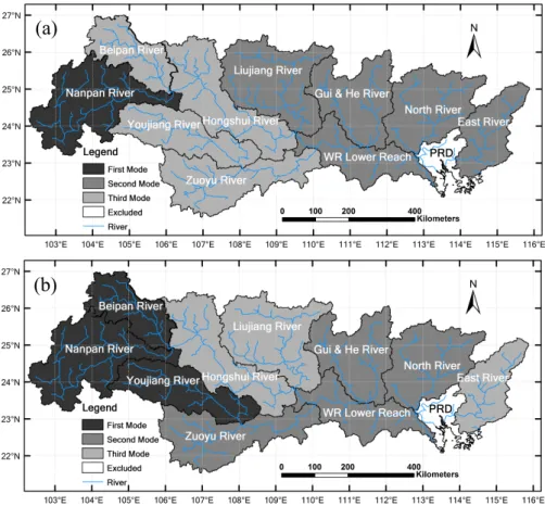
Over the Pearl River basin, there are mainly three types of precipitation events: frontal type storms (during April–June), tropical cyclonic rains (during July–October), and convective rainstorms (during June–August) (Niu, 2013). Therefore, the rainy season essentially lasts for 7 months in a year, from April to October (Niu, 2010). This high variability of pre-cipitation is partly transferred to the high runoff variabil-ity at the timescale of 0.59 yr (see Fig. 3a). Apart from the high variability for less-than 1 yr periods, the variability in the dominant low-frequency variability band (DLVB), 0.83– 5.21 yr, demonstrates the distinct features of the three multi-scale variability modes in the Pearl River basin (see Fig. 3a). The DLVB is determined as follows: the local dominant vari-ability band is defined as the longest projecting portion with its peak spectrum at least above the mean red-noise spectrum and most likely to reach a higher confidence level (e.g., 95 % level); and the DLVB is the band that covers most of the iden-tified dominant variability bands of the 10 sub-basins. The three coherent modes of soil moisture in Fig. 3b show that the variability at longer timescales (longer than 0.59 yr) has the striking features within the DLVB range of 1.92–5.21 yr. Figure 4a and b shows the sub-basin clusters of multiscale variability of runoff and soil moisture, respectively; the three clusters correspond to the three coherent modes. The cluster of runoff is basically consistent with that of precipitation (see Niu, 2010), while the cluster of soil moisture displays dis-similar results. One rainstorm center in the Pearl River basin is located in the lower reach of the Hongshui River basin (Pearl River Water Resources Commission, 2005), and this results in the highest power at the 0.5–1 yr period for the third mode of precipitation and runoff in the central part. The Nan-pan River basin is in the northwest region of the Pearl River basin. This region has the highest altitudes, and is influenced
0.25 0.5 1 2 4 8 -3 -2 -1 0 1 2 3 4 Period (years) S ta n da rd ized w a vel et pow er DLVB 0.59 yr (a) 0.25 0.5 1 2 4 8 -3 -2 -1 0 1 2 3 4 Period (years) S ta n dar d ized w a vel et pow er 0.59 yr DLVB (b)
Fig. 3. (a) Coherent modes of temporal variability for the wavelet power spectrum of monthly runoff anomaly over the Pearl River basin. The bold line is the first mode, while the line with circles and the dashed line are the second mode and the third mode, respectively. DLVB stands for the dominant low-frequency variability band (0.83– 5.21 yr). (b) Same with (a) but for soil moisture with DVLB (1.92–5.21 yr).
Fig. 3. (a) Coherent modes of temporal variability for the
wavelet-power spectrum of monthly runoff anomaly over the Pearl River basin. The bold line is the first mode, while the line with circles and the dashed line are the second mode and the third mode, re-spectively. DLVB stands for the dominant low-frequency variabil-ity band (0.83–5.21 yr). (b) Same with (a) but for soil moisture with DLVB (1.92–5.21 yr).
by the topographic rain shadow with respect to the prevail-ing storm tracks. The east region of the Pearl River basin is close to the South China Sea, and is subjected to convective movement of water by semitropical typhoons (Niu, 2013). The higher variability in the 1–4 yr band is more obvious, compared to the third mode of runoff in the central part of the Pearl River basin.
The Beipan, Nanpan, and Youjiang river basins, located in the northwestern region with the highest altitudes, be-long to the first mode of soil moisture that displays a single peak of high variability at longer timescales. In these basins, the high-frequency precipitation variability is kept less by runoff and reflected more by soil moisture at low frequen-cies. The second mode of soil moisture, including the North, Guihe, and Zuoyu river basins and the West River’s lower reach, shows relatively flat variability power distribution (see Fig. 3b), which either has lower altitudes or is located at the downstream of the Pearl River. Meanwhile, the third mode of soil moisture, to which the Liujiang, Hongshui and East river basins belong, sits between the above two distinctive modes, which is partly consistent with elevation variations between the other two modes.
(b)
(a)
Fig. 4.
(a) Spatial distribution of coherent modes (in Fig. 3) on global wavelet
spectrum of runoff. (b) Same as (a) but for soil moisture.
Fig. 4. (a) Spatial distribution of coherent modes (in Fig. 3) on global wavelet spectrum of runoff. (b) Same as (a) but for soil moisture.
4.3 Evolution of bandpass variance
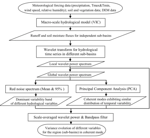
To highlight the variability processes with respect to time for the coherent mode of GWS, the variance evolution in the dominant band is inspected by using the scale-averaged wavelet power and bandpass-filtered time series. Figure 5 il-lustrates the flowchart of unfolding regional variance evolu-tion of hydrological variables. We use Eq. (6) to compute the scale-averaged wavelet power, and Eq. (7) to generate the bandpass-filtered series. The representative of each mode is the time series average of the independent sub-basins that belong to the same mode.
Figure 6 shows the runoff series of both scale-averaged wavelet power and corresponding bandpass-filtered time se-ries for three coherent modes between the timescales of 0.83 and 5.21 yr. The second mode (i.e., the East River, North River, Guihe River, and Liujiang river basins and the WR’s (West River’s)lower reach) shows larger variance processes in terms of the magnitude of average variance (2508 mm2), with high variance occurring sometime around 1963, and also two other periods from 1983 to 1984 and from 1991 to 1996. The variability processes for the third mode (i.e., the Hongshui, Beipan, Youjiang and Zuoyu river basins) show an irregular cycle of an increasing amplitude of runoff events
followed by a decreasing amplitude. The approximately 5 yr cycle is also clearly apparent from 1967 to 1977 and from 1987 to 1997.
Figure 7 shows the variance evolution of soil moisture within 1.92–5.21 yr. Compared to the results obtained for runoff, the soil moisture variability processes are relatively smooth along the time and relatively balanced in terms of the magnitude of average variance for the three modes (i.e., 792, 1151 and 911 mm2). A large variance can be identified for the first mode (i.e., the Beipan, Nanpan and Youjiang river basins) for the period 1955–1970. The variance processes for the second mode (i.e., the North, Guihe and Zuoyu river basins and the WR’s lower reach) are relatively gentle, while the third mode (i.e., the East, Liujiang and Hongshui river basins) shows noticeable changes with two high-variance pe-riods: 1960–1970 and 1995–2000.
4.4 Teleconnection to climatic patterns
To examine the possible linkages of climatic patterns with variations in runoff and soil moisture in the Pearl River basin, their wavelet coherences are inspected. The results are pre-sented below.
Dominant variability band of different hydrological variables
Coherent modes exhibiting similar distribution of temporal variability
Scale-averaged wavelet power & Bandpass filter
Variance evolution of different variables for the region (sub-basins) in coherent mode
Meteorological forcing data (precipitation, Tmax&Tmin, wind speed, relative humidity); soil and vegetation data; DEM data
Local wavelet power spectrum
Runoff and soil moisture fluxes for independent sub-basins
Wavelet transform for hydrological time series in different sub-basins
Red noise spectrum (Mean & 95% )
Global wavelet power spectrum
Principal Component Analysis (PCA) Macro-scale hydrological model (VIC)
Fig. 5. The flowchart of regional variance evolutions for different hydrological variables.
Fig. 5. The flowchart of regional variance evolutions for different hydrological variables.
4.4.1 Runoff
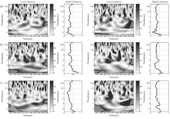
Figure 8 shows the local and global wavelet coherence of the three modes of runoff (modes one to three, from top to bottom) in the Pearl River basin with ENSO (left panels) and IOD (right panels). It is observed that, for the first-mode runoff and ENSO (Fig. 8a, left panel), there are significant regions around the 1 yr band within the periods 1970–1975 and 1990–1995, and also for the 2–4 yr band around 1995. The vectors in the regions outlined by thick contours in-dicate the close in-phase relationship around 1995 (for 2– 4 yr band), which is also consistent with the rank correlation results in Sect. 4.5. These observations seem to indicate a link (i.e., close in-phase variance change) between the first-mode runoff and ENSO in the 2–4 yr band around 1995. The right panel in Fig. 8a shows the correlations of the first-mode runoff and IOD. The noticeable in-phase relations are found within the 2–4 yr band around 1995.
The runoff in the eastern part of the Pearl River basin belongs to the second coherent mode. Its correlation with ENSO is shown in Fig. 8b (left panel). The identifiable correlations (i.e., the time–frequency region is with signif-icant wavelet coherence) are within the 1–4 yr band during the 1970–1975 period and around 1983, and within the 2– 4 yr band around 1995. The phase relations indicate ENSO
leading the second-mode runoff during the 1970–1975 pe-riod. The in-phase relation is identified within the 2–4 yr band around 1995. For the correlations between the second-mode runoff and IOD in Fig. 8b (right panel), the identifi-able correlations are mainly within the 0.5–2 yr band around 1983 (anti-phase) and within the 1–4 yr band around 1995 (in-phase).
The left panel in Fig. 8c shows that the identifiable correla-tion between the third-mode runoff and ENSO exists around the 4 yr band during the period 1985–1995. The vectors in the regions show close in-phase relations of variance pro-cesses. Figure 8c (right panel) shows the main identifiable correlations between the third-mode runoff and IOD, with anti-phase relations within the 1–2 yr band during the period 1970–1975 and in-phase relations within the 2–4 yr band dur-ing the period 1990–1995. The global wavelet coherence re-sults in Fig. 8 also show the oscillation correlation around the 1–6 yr band, especially between the second and third modes of runoff and IOD (the right panels in Fig. 8b and c).
4.4.2 Soil moisture
The wavelet coherence between the first-mode soil mois-ture and ENSO in Fig. 9a (right panel) discloses high co-herence at both short and relatively longer periods. The
19520 1955 1960 1965 1970 1975 1980 1985 1990 1995 2000 0.1 0.2 0.3 0.4 0.5 0.6 0.7 0.8 0.91 Streamflow 19520 1955 1960 1965 1970 1975 1980 1985 1990 1995 2000 0.1 0.2 0.3 0.4 0.5 0.6 0.7 0.8 19520 1955 1960 1965 1970 1975 1980 1985 1990 1995 2000 0.1 0.2 0.3 0.4 0.5 0.6 0.7 0.8 σ 2 σ 2 σ 2 Runoff
Fig. 6.
The scale-averaged (0.83–5.21 yr) wavelet power for runoff (thick black curve)
and the bandpass filtered time series of square form (runoff
2) (thin curve) from 0.83 to
5.21 yr using a wavelet filter. The upper, middle and lower panels are the first, second
and third modes of runoff, respectively. The black shading indicates positive peaks in
the filtered time series, while the white are negative peaks. The time series of the
wavelet power and the bandpass filtered (before squaring) are the averaged time series
over the sub-basins belonging to the same mode. The averaged variances of initial
monthly runoff time series
2for the first, second and third modes are 263.26 mm
2,
2,507.64 mm
2and 1,096.32 mm
2, respectively.
Fig. 6. The scale-averaged (0.83–5.21 yr) wavelet power for runoff (thick black curve) and the bandpass filtered time series of square form
(runoff squared) (thin curve) from 0.83 to 5.21 yr using a wavelet filter. The upper, middle and lower panels are the first, second and third modes of runoff, respectively. The black shading indicates positive peaks in the filtered time series, while the white are negative peaks. The wavelet power and bandpass filtered time series (before squaring) are the averaged time series over the sub-basins belonging to the same mode. The averaged variances of initial monthly runoff time seriesσ2for the first, second and third modes are 263.26, 2507.64 and 1096.32 mm2, respectively. 19520 1955 1960 1965 1970 1975 1980 1985 1990 1995 2000 0.1 0.2 0.3 0.4 0.5 0.6 0.7 0.8 Soil moisture 19520 1955 1960 1965 1970 1975 1980 1985 1990 1995 2000 0.1 0.2 0.3 0.4 0.5 0.6 1952 1955 1960 1965 1970 1975 1980 1985 1990 1995 2000 0 0.1 0.2 0.3 0.4 0.5 0.6 σ 2 σ 2 σ 2
Fig. 7.
Same to Fig. 5, but for soil moisture in 1.92–5.21 yr band. The averaged
variances of initial monthly soil moisture time series
2for the first, second and third
modes are 792.45 mm
2, 1,151.50 mm
2and 911.17 mm
2, respectively.
Fig. 7. Same as Fig. 5, but for soil moisture in the 1.92–5.21 yr band. The averaged variances of initial monthly soil moisture time seriesσ2 for the first, second and third modes are 792.45, 1151.50 and 911.17 mm2, respectively.
major identifiable correlations are distributed within the 1– 2 yr band (around 1965 and 1973, and during the period 1990–1995), the 2–4 yr band (around 1995), and the 4 yr band (during the period 1980–1990). The results also show close in-phase relationships for the regions during the pe-riod 1980–1990 and around 1995. The major identifiable
correlations between the first-mode soil moisture and IOD in Fig. 9a (right panel) are found within the 1–2 yr band around 1975 (anti-phase), and within the 2–4 yr band around the pe-riod 1990–1995 (close in-phase).
The left panel in Fig. 9b shows that the identifiable correla-tions between the second mode of soil moisture and ENSO,
Fig. 8.
(a) Squared wavelet coherence (local and global) between the first mode runoff
and ENSO time series (left panel), and between the first mode runoff and IOD time
series (right panel). The 5% significance level against red noise is shown as a thick
contour and the cone of influence (COI) where edge effects might become important
is shown as a thin black line. The relative phase relationship is shown as arrows (with
in-phase pointing right, anti-phase pointing left, runoff leading ENSO by 90° pointing
straight down, and ENSO leading runoff pointing straight up). (b) Same as (a) but for
the second model of runoff. (c) Same as (a) but for the third model of runoff.
Fig. 8. (a) Squared wavelet coherence (local and global) of the first mode runoff and ENSO time series (left panel), and between the first
mode runoff and IOD time series (right panel). The 5 % significance level against red noise is shown as a thick contour and the cone of influence (COI) where edge effects might become important is shown as a thin black line. The relative phase relationship is shown as arrows (with in-phase pointing right, anti-phase pointing left, runoff leading ENSO by 90◦pointing straight down, and ENSO leading runoff pointing straight up). (b) Same as (a) but for the second model of runoff. (c) Same as (a) but for the third model of runoff.
which are basically distributed within the 1–4 yr band, in-cluding around 1965 (1–2 yr band), 1974 (2 yr), 1976 (1 yr), 1983 (1–2 yr band), 1993 (1–2 yr band), and 1995 (2–4 yr band). The vectors in the regions show that ENSO leads soil moisture around 1965 and in-phase relations around 1983. In Fig. 9b (left panel), they are within the 0.5–2 yr band dur-ing the period 1980–1985 (anti-phase) and within the 2–4 yr band around 1995 (close in-phase).
The identifiable correlations between the third mode of soil moisture and ENSO in Fig. 9c (left panel) can be found within the 1–2 yr band during the period 1960–1975 and the 1–4 yr band during the period 1990–2000, in which the vec-tors indicate that ENSO leads soil moisture in the former region and close in-phase relations in the latter region. The right panel in Fig. 9c shows that the major identifiable corre-lations are within the 0.5–2 yr band during the period 1980– 1985 (anti-phase) and within the 1–4 yr band during the pe-riod 1990–2000 (close in-phase). The global wavelet coher-ence in Fig. 9b and c shows the teleconnection peaks between regional (the eastern and central parts) soil moisture and cli-matic patterns at longer timescales.
4.5 Correlation at multiple timescales
As indicated above, the significant correlations of runoff and soil moisture with the two climatic patterns (ENSO and IOD) mainly exist within the DLVB. To highlight the teleconnec-tion influences further, the correlateleconnec-tions of wavelet power time series between a hydrological variable and a climatic in-dex, within the corresponding DLVB, are computed by using Spearman’s rank correlation. A positive correlation value in-dicates that the amplitudes of variance over the desired time period have consistent evolution processes, while a negative correlation value corresponds to opposite evolution processes (Niu, 2010).
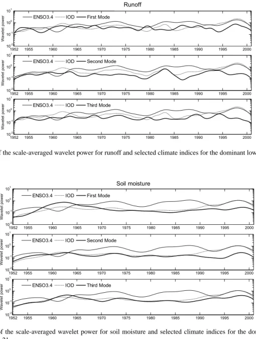
Figure 10 shows the scale-averaged wavelet power for each runoff mode within the 0.83–5.21 yr band and the two climatic indices (i.e., ENSO and IOD), and Table 3 lists the corresponding correlation results. It is observed that the first and third modes of runoff correlate with ENSO and IOD oc-casionally for the divided 10 yr periods. The second mode of runoff is basically depicted by IOD, which is reflected by the significant correlations for all the divided periods and
Fig. 9.
Same as Fig. 8 but for soil moisture.
Fig. 9. Same as Fig. 8 but for soil moisture.
also by the high correlation value of 0.643 for the complete time period (1952–2000). The opposite evolution processes are found for ENSO and IOD for the period 1960–1969 (see Fig. 10), which, in turn, produces positive correlations (0.295 and 0.744) and negative correlations (−0.417 and−0.501) with the first and second modes of runoff, respectively. This also confirms the different temporal processes of variance for the two climatic patterns (Niu, 2013). Figure 11 indicates a good relationship between each mode of soil moisture and IOD within the 1.92–5.21 yr band for the entire period, with the rank correlation values of 0.669 (for the first mode), 0.319 (for the second mode) and 0.832 (for the third mode), as pre-sented in Table 3. Significant correlations are also found be-tween soil moisture and ENSO for most of the divided 10 yr periods, but with lower correlation degree for the first mode of soil moisture (i.e., in the western part of the basin) and higher for the second mode (i.e., in the eastern part of the basin) after the 1970s, compared to the corresponding corre-lation level between soil moisture and IOD.
5 Inferences on droughts and floods
To illustrate the potential utility of the above analysis, possible inferences of the results as to the occurrence of
basin-featured extreme hydrological events (i.e., the flood event in 1994 and the drought event in 1963) are explored.
Two Asian monsoon systems, namely the Indian summer monsoon and the East Asian summer monsoon, strongly in-fluence eastern China (Ding and Chan, 2005). Torrence and Webster (1999) discussed the relationship between the In-dian monsoon and ENSO, through analysis of a 122 yr-long data set (1872–1993). They reported that the Indian mon-soon tends to be weaker during the El Niño event periods and that the weak monsoon statistically leads by about 4 months to the peak of equatorial Pacific SST. A strong soon is associated with cold SST, and its peak lags the mon-soon by about 4 months (Torrence and Webster, 1999). Even though investigating the mechanisms and relationships be-tween climatic indices and monsoon systems is out of the scope of the current study, the results reported by Torrence and Webster (1999) are helpful for understanding the coher-ence results obtained in the present study. The complex cor-relations between monsoon and climatic indices indicate a phase difference of the variability of runoff or soil moisture with climatic signals.
1952 1955 1960 1965 1970 1975 1980 1985 1990 1995 2000 10-2 10-1 100 101 Wa ve le t p o w er Streamflow 1952 1955 1960 1965 1970 1975 1980 1985 1990 1995 2000 10-2 10-1 100 101 Wa ve le t p o w er 1952 1955 1960 1965 1970 1975 1980 1985 1990 1995 2000 10-2 10-1 100 101 Wa ve le t p o w er
ENSO3.4 IOD First Mode
ENSO3.4 IOD Second Mode
ENSO3.4 IOD Third Mode
Runoff
Fig. 10. Comparison of the scale-averaged wavelet power for runoff and selected
climate indices for the dominant low-frequency variability band 0.83–5.21 yr.
Fig. 10. Comparison of the scale-averaged wavelet power for runoff and selected climate indices for the dominant low-frequency variability
band 0.83–5.21 yr. 1952 1955 1960 1965 1970 1975 1980 1985 1990 1995 2000 10-2 10-1 100 101 Wa ve le t p o w er Soil moisture 1952 1955 1960 1965 1970 1975 1980 1985 1990 1995 2000 10-2 10-1 100 101 Wave le t p o w er 1952 1955 1960 1965 1970 1975 1980 1985 1990 1995 2000 10-2 10-1 100 101 Wav el e t p o w er
ENSO3.4 IOD First Mode
ENSO3.4 IOD Second Mode
ENSO3.4 IOD Third Mode
Fig. 11.
Comparison of the scale-averaged wavelet power for soil moisture and
selected climate indices for the dominant low-frequency variability band 1.92–5.21 yr.
Fig. 11. Comparison of the scale-averaged wavelet power for soil moisture and selected climate indices for the dominant low-frequency
variability band 1.92–5.21 yr.
5.1 Flood event
In 1994, a major flood occurred over almost the entire Pearl River basin. This flood event offers a reasonable basis to interpret the results from the wavelet analysis in the con-text of relationships that exist between large-scale climatic patterns and basin-featured hydrological processes. The sig-nificant common wavelet power and coherence in Fig. 8a and c show strong in-phase relations between runoff and IOD within the 2–4 yr band in 1994, but the correlation of runoff with ENSO is not that visible; it is relevant to note that there was a strong positive IOD event in 1994. Further, in 1994, the moisture transport resulting from the southeastern trop-ical Indian Ocean gave rise to an enhanced convection over the Indian subcontinent and East Asia (Behera et al., 1999).
Therefore, heavy rainfall and flood occurred over southern China, including in the Pearl River basin.
The impactful occurrence of small-scale activity (variabil-ity) is indeed often supported by larger-scale activity (see Kumar, 1996 for details). Flood events normally occur in response to abundant precipitation over a short period of time, especially when the land has already been in a wet state (runoff or soil moisture) over a long time period. The abundant precipitation in 1994 occurred during an already wet state that existed due to high runoff in the basin before 1994, including due to high runoffs in the central part in 1992 and 1993 (shown in Fig. 6b) and in the western part in 1993 (shown in Fig. 6c), thus resulting in an extreme flood over the whole basin in 1994. Although abundant precipitation also
Table 3. Spearman’s rank correlations between the wavelet powers of runoff/soil moisture and selected climate indices in the low-frequency
dominant variability band. DOF denotes the degrees of freedom. Bold indicates greater than 95 % confidence level.
52–59 60s 70s 80s 90s 1952–2000
Runoff DOF 38 46 46 46 46 214
(0.83–5.21 yr) First mode
ENSO −0.430 −0.417 0.210 0.100 0.874 0.289 IOD −0.184 0.295 0.167 −0.458 0.502 0.158 Second mode ENSO 0.371 −0.501 0.866 −0.098 −0.855 0.009 IOD 0.876 0.744 0.896 0.721 −0.538 0.643 Third mode ENSO −0.362 −0.005 0.696 0.526 −0.595 −0.068 IOD 0.016 −0.152 0.705 0.241 −0.435 0.239
Soil moisture DOF 18 21 21 21 21 93
(1.92–5.21 yr) First mode
ENSO 0.438 −0.859 0.545 0.433 0.417 −0.160 IOD 0.995 0.877 0.719 0.770 0.529 0.669 Second mode ENSO 0.462 −0.709 0.887 0.585 0.886 0.174 IOD 0.991 0.893 0.774 0.364 0.649 0.319 Third mode ENSO 0.438 −0.661 0.556 −0.511 0.632 0.094 IOD 0.996 0.767 0.519 −0.276 0.903 0.832
occurred around 1983, it did not cause any major flood since the land surface was not as wet during the period before 1983 as it was before 1994, as the second mode of runoff indi-cates. Further, the soil moisture condition before 1983 was also in a long-term dry state (see Fig. 7), especially for the first and the third modes of soil moisture. Such relatively dry runoff and soil moisture states play a significant role in low-ering and slowing down the runoff over the basin and, con-sequently, the resulting flow would not be sufficient to cause major floods; the fact that there was no flood in 1983 despite abundant precipitation explains this.
5.2 Drought event
In 1963, about 5 % of the total area of the Pearl River basin was subjected to a severe drought; this drought also pro-vides a reasonable basis for interpreting the results from the wavelet analysis above. As seen in Fig. 9, the soil mois-ture (especially for the second and third modes) has signif-icant wavelet coherence at >95 % confidence levels with the ENSO, but not IOD, within the 1–2 yr band around 1963; ENSO was in a weak warm phase (El Niño) in that year. Statistically, a weak Indian monsoon may be related to an El Niño period (Torrence and Webster, 1999). How-ever, the lower SST during summer in the tropical Pacific,
the weaker the convective activities may be around southern China (Huang and Wu, 1989). Both these conditions might have been responsible for the limited precipitation over the Pearl River basin in 1963 and, consequently, for the severe drought in the basin.
It is observed that soil moisture was in a dry condition around 1963 (see Fig. 7). The general geographic feature of the Pearl River basin is that elevation decreases from the northwest to the southeast. Moreover, the insufficient precip-itation condition in 1963 is also noticeable downstream of the Pearl River (Niu, 2013). The precipitation deficit in conjunc-tion with the basin geography features are responsible for the serious dry state in both the northwestern and the southeast-ern parts, resulting in the severe drought in 1963 over the basin. Drought events normally occur when precipitation is insufficient over a long period (or even a short one) in an al-ready dry state of soil moisture over a long time period. The precipitation deficit in 1989 is comparable to that in 1963, es-pecially for the first and third modes (Niu, 2010). However, the long-term dry condition around 1989 is not comparable to that around 1963 (see Fig. 7). Therefore, the probability of a severe drought event occurrence in 1989 was less than in 1963, as the long-term dry condition around 1963 is more noticeable.
6 Conclusions
In this study, VIC-model-simulated runoff and soil moisture data over the Pearl River basin, southern China, were ana-lyzed using wavelets to examine the teleconnections between such processes and two large-scale climatic patterns, ENSO and IOD. The results indicate that the hydrological variabili-ties in the basin have undergone considerable changes in vari-ance and coherence with these two climatic patterns over the study period 1952–2000.
The wavelet power spectrum shows that the distinctive mode of runoff variability is dominant at the low-frequency band (DLVB) of 0.83–5.21 yr. The bandpass-filtered time se-ries displays the intervals of high or low variance for dif-ferent coherent regions in the basin. The variance evolution of runoff is essentially influenced by IOD, especially for the second and third modes (i.e., the eastern and the central parts of the basin), according to the rank correlation analysis for the scale-averaged wavelet power series. In addition, the sec-ond mode of runoff in the eastern part of the basin displays more significant coherence with ENSO within the DLVB.
The soil moisture at the headwater basin area (i.e., regions with relatively high altitudes) shows an isolated high vari-ability at longer timescales (2–4 yr), which is well correlated with the low-frequency variability of IOD for both the di-vided 10 yr periods and the total studied period (49 yr). The soil moisture has the capability to memorize the variability of climatic signals, as had previously been demonstrated (Chen and Kumar, 2002). This capability of soil moisture results in more significant wavelet-based correlations at relatively longer timescales when compared to those for runoff.
The identifiable relations with significant coherence at >95 % confidence level in a time–frequency domain suggest that the variability in local runoff and soil moisture variabil-ity is triggered by large-scale atmospheric circulation and in-fluenced by climatic patterns. These underlying correlations, coupled with the bandpass-filtered time series of hydrolog-ical variables, provide valuable information to draw infer-ences regarding the occurrence of basin-featured extreme hydrological events (i.e., flood or drought). Such an under-standing, as evidenced by the current study, is paramount for providing skillful long-term prediction of hydrological pro-cesses for large-scale river basins (such as the Pearl River basin) that are of interest at national, and even international, levels. With increasing concerns on the impacts of global cli-mate change on our water resources in the future (see, for instance, Sivakumar, 2011, for a more recent account), this understanding becomes all the more important.
Acknowledgements. This research was supported by two Hong
Kong RGC GRF projects (no.: HKU 710712E and HKU 710910E) and one small project (no.: 201209176068) from the University of Hong Kong. Bellie Sivakumar acknowledges the financial support from the Australian Research Council (ARC) through the Future Fellowship grant (FT110100328). Wavelet software implemented
here are provided by C. Torrence and G. P. Compo and available on http://paos.colorado.edu/research/wavelets/. The Matlab package prepared by A. Grinsted, J. C. Moore, and S. Jevrejeva is available at http://noc.ac.uk/using-science/crosswavelet-wavelet-coherence. Many thanks to Editor Bettina Schaefli and two anonymous reviewers, for the thorough review and helpful comments, which helped improve an earlier version of this manuscript.
Edited by: B. Schaefli
References
Asquith, D.: Learning to live with statistics: from concept to prac-tice, Lynne Rienner, Boulder, Colorado, 2008.
Behera, S. K., Krishnan, S., and Yamagata, T.: Unusual ocean-atmosphere conditions in the tropical Indian Ocean during 1994, Geophys. Res. Lett., 26, 3001–3004, 1999.
Chen, J. and Kumar, P.: Role of terrestrial memory in modulating ENSO impacts in North America, J. Climate, 15, 3569–3585, 2002.
Chen, J. and Kumar, P.: A modelling study of the ENSO influence on the terrestrial energy profile in North America, J. Climate, 17, 1657–1670, 2004.
Chen, Y. D., Zhang, Q., Lu, X. X., Zhang, S. R., and Zhang, Z. X.: Precipitation variability (1956–2002) in the Dongjiang River (Zhujiang River basin, China) and associated large-scale circula-tion, Quatern. Int., 244, 130–137, 2011.
Cosby, B. J., Hornberger, G. M., Clapp, R. B., and Ginn, T. R.: A statistical exploration of the relationships of soil moisture char-acteristics to the physical properties of soils, Water Resour. Res., 20, 682–690, 1984.
Cui, W. Z., Chen, J., Wu, Y. P., and Wu, Y. D.: An overview of water resources management of the Pearl River, Water Sci. Technol., 7, 101–113, 2007.
Ding, Y. and Chan, J. C. L.: The East Asian summer monsoon: an overview, Meteorol. Atmos. Phys., 89, 117–142, 2005.
Dümenil, L. and Todini, E.: A rainfall-runoff scheme for use in the Hamburg climate model, in: Advances in theoretical hydrology, A tribute to James Dooge, Eur. Geophys. Soc. Ser. Hydrol. Sci., vol. 1, edited by: O’Kane, P., Elsevier Sci., New York, 129–157, 1992.
Eltahir, E. A. B.: El Niño and the natural variability in the flow of the Nile River, Water Resour. Res., 32, 131–137, 1996. Farge, M.: Wavelet transforms and their applications to turbulence,
Annu. Rev. Fluid Mech., 24, 395–457, 1992.
Feng, S., Hu, Q., and Qian, W. H.: Quality control of daily mete-orological data in China, 1951–2000: A new dataset, Int. J. Cli-matol., 24, 853–870, 2004.
Fischer, T., Gemmer, M., Liu, L., and Jiang, T.: Change-points in climate extremes in the Zhujiang River Basin, South China, 1961–2007, Climatic Change, 110, 783–799, doi:10.1007/s10584-011-0123-8, 2012.
Grinsted, A., Moore, J. C., and Jevrejeva, S.: Application of the cross wavelet transform and wavelet coherence to geophys-ical time series, Nonlin. Processes Geophys., 11, 561–566, doi:10.5194/npg-11-561-2004, 2004.
Guan, Z. and Yamagata, T.: The unusual summer of 1994 in East Asia: IOD Teleconnections, Geophys. Res. Lett., 30, 1544, doi:10.1029/2002GL016831, 2003.
Hansen, M. C., DeFries, R. S., Townshend, J. R. G., and Sohlberg, R.: Global land cover classification at 1 km spatial resolution us-ing a classification tree approach, Int. J. Remote Sens., 21, 1331– 1364, 2000.
Huang, R. H. and Wu, Y. F.: The influence of ENSO on the summer climate change in China and its mechanism, Adv. Atmos. Sci., 6, 21–23, 1989.
Kumar, P.: Role of coherent structure in the stochastic dynamic variability of precipitation, J. Geophys. Res., 101, 26393–26404, 1996.
Kumar, P. and Foufoula-Georgiou, E.: Wavelet analysis for geo-physical applications, Rev. Geophys., 35, 385–412, 1997. Labat, D.: Oscillations in land surface hydrological cycle, Earth
Planet. Sc. Lett., 242, 143–154, 2006.
Labat, D.: Cross wavelet analyses of annual continental freshwater discharge and selected climate indices, J. Hydrol., 385, 269–278, 2010a.
Labat, D.: Wavelet analyses in hydrology, in: Advances in Data-Based Approaches for Hydrologic Modeling and Forecasting, edited by: Sivakumar, B. and Berndtsson, R., World Scientific Publishing Company, Singapore, 371–410, 2010b.
Li, C. Y. and Zhou, W.: Changes in western Pacific tropical cy-clones associated with the El Niño-southern oscillation cycle, J. Climate, 25, 5864–5878, doi:10.1175/JCLI-D-11-00430.1, 2012. Liang, X., Lettenmaier, D. P., Wood, E. F., and Burges, S. J.: A simple hydrologically based model of land surface water and en-ergy fluxes for general circulation models, J. Geophys. Res., 99, 14415–14428, 1994.
Maraun, D. and Kurths, J.: Cross wavelet analysis: significance testing and pitfalls, Nonlin. Processes Geophys., 11, 505–514, doi:10.5194/npg-11-505-2004, 2004.
Maraun, D., Kurths, J., and Holschneider, M.: Nonstationary Gaussian processes in wavelet domain: Synthesis, estima-tion, and significance testing, Phys. Rev. E, 75, 016707, doi:10.1103/PhysRevE.75.016707, 2007.
Markovi´c, D. and Koch, M.: Wavelet and scaling analysis of monthly precipitation extremes in Germany in the 20th cen-tury: Interannual to interdecadal oscilliations and the North At-lantic Oscillation influence, Water Resour. Res., 41, W09420, doi:10.1029/2004WR003843, 2005.
Maurer, E. P., Wood, A. W., Adam, J. C., and Lettenmaier, D. P.: A long-term hydrologically based dataset of land surface fluxes and states for the conterminous United States, J. Climate, 15, 3237– 3251, 2002.
Moriasi, D. N., Arnold, J. G., Van Liew, M. W., Bingner, R. L., Harmel, R. D., and Veith, T. L.: Model evaluation guidelines for systematic quantification of accuracy in watershed simulations, T. ASABE, 50, 885–990, 2007.
Nijssen, B., Lettenmaier, D. P., Liang, X., Wetzel, S. W., and Wood, E. F.: Streamflow simulation for continental-scale river basins, Water Resour. Res., 33, 711–724, 1997.
Nijssen, B., Schnur, R., and Lettenmaier, D. P.: Global retrospective estimation of soil moisture using the VIC land surface model, J. Climate, 14, 1790–1808, 2001a.
Nijssen, B., O’Donnell, G. M., Lettenmaier, D. P., Lohmann, D., and Wood, E. F.: Predicting the discharge of global rivers, J. Cli-mate, 14, 3307–3323, 2001b.
Niu, J.: A comprehensive analysis of terrestrial hydrological pro-cesses over the Pearl River basin in South China, Ph.D. thesis, Univ. of Hong Kong, Hong Kong, 202 pp., 2010.
Niu, J.: Precipitation in the Pearl River basin, South China: Scaling, regional patterns, and influence of large-scale climate anomalies, Stoch. Env. Res. Risk A., 27, 1253–1268, doi:10.1007/s00477-012-0661-2, 2013.
Niu, J. and Chen, J.: Application of VIC and routing scheme to Pearl River basin in south China, in: Advance in Water Resources and Hydraulic Engineering, Proc. 16th IAHR-APD Congress and 3rd Symposium of IAHR-ISHS, 20–23 October 2008, Hohai Univ., Nanjing, China, 72–76, doi:10.1007/978-3-540-89465-0_14, 2009.
Niu, J. and Chen, J.: Terrestrial hydrological features of the Pearl River basin in southern China, J. Hydro-Environ. Res., 4, 279– 288, doi:10.1016/j.jher.2010.04.016, 2010.
Özger, M., Mishra, A. K., and Singh, V. P.: Low frequency drought variability associated with climatic indices, J. Hydrol., 364, 152– 162, 2009.
Pearl River Hydraulic Research Institute: Drought monitor and as-sessment reports for the Pearl River basin using remote sensing, Pearl River Hydraulic Research Institute, Guangzhou, 60 pp., 2007.
Pearl River Water Resources Commission: Pearl Rive flood pre-vention handbook, Pearl River Water Resources Commission, Guangzhou, 150 pp., 2005.
Saji, N. H., Goswami, B. N., Vinayachandran, P. N., and Yamagata, T.: A dipole mode in the tropical Indian Ocean, Nature, 401, 360– 363, 1999.
Schaefli, B. and Zehe, E.: Hydrological model performance and pa-rameter estimation in the wavelet-domain, Hydrol. Earth Syst. Sci., 13, 1921–1936, doi:10.5194/hess-13-1921-2009, 2009. Schaefli, B., Maraun, D., and Holschneider, M.: What drives high
flow events in the Swiss Alps? Recent developments in wavelet spectral analysis and their application to hydrology, Adv. Water Resour., 30, 2511–2525, 2007.
Sheffield, J., Goteti, G., Wen, F. H., and Wood, E. F.: A simulated soil moisture based drought analysis for the United States, J. Geophys. Res., 109, D24108, doi:10.1029/2004JD005182, 2004. Sivakumar, B.: Global climate change and its impacts on water re-sources planning and management: assessment and challenges, Stoch. Environ. Res. Risk A., 25, 583–600, 2011.
Todini, E.: The ARNO rainfall-runoff model, J. Hydrol., 175, 339– 382, 1996.
Torrence, C. and Compo, G. P.: A practical guide to wavelet analy-sis, B. Am. Meteorol. Soc., 79, 61–78, 1998.
Torrence, C. and Webster, P. J. Interdecadal changes in the ENSO-Monsoon system, J. Climate, 12, 2679–2690, 1999.
Trenberth, K. E. and Stepaniak, D. P.: Indices of El Niño evolution, J. Climate, 14, 1697–1701, 2001.
Troy, T. J., Wood, E. F., and Sheffield, J.: An efficient calibration method for continental-scale land surface modeling, Water Re-sour. Res., 44, W09411, doi:10.1029/2007WR006513, 2008. Verdin, K. L. and Verdin, J. P.: A topological system for delineation
and codification of the Earth’s river basins, J. Hydrol., 218, 1–12, 1999.
Wu, Y. and Chen, J.: An operation-based scheme for a multiyear and multipurpose reservoir to enhance macro-scale hydrologic models, J. Hydrometeorol., 13, 270–283, 2012.
Yang, T., Shao, Q. X., Hao, Z. C., Chen, X., Zhang, Z. X., Xu, C. Y., and Sun, L. M.: Regional frequency analysis and spatio-temporal pattern characterization of rainfall extremes in the Pearl River Basin, China, J. Hydrol., 380, 386–405, 2010.
Zhang, Q., Xu, C. Y., Jiang, T., and Wu, Y. J.: Possible influence of ENSO on annual maximum streamflow of Yangtze River, China, J. Hydrol., 333, 265–274, 2007.
Zhang, Q., Xu, C. Y., Yu, Z. G., Liu, C. L., and Chen, Y. D.: Mul-tifractal analysis of streamflow records of the East River basin (Pearl River), China, Physica A, 388, 927–934, 2009.
Zhang, Q., Xu, C. Y., Zhang, Z. X., and Chen, Y. Q.: Changes of atmospheric water vapor budget in the Pearl River basin and pos-sible implications for hydrological cycle, Theor. Appl. Climatol., 102, 185–195, 2010.
Zhang, Q., Singh, V. P., Peng, J. T., Chen, Y. Q., and Li, J. F.: Spatial-temporal changes of precipitation structure across the Pearl River basin, China, J. Hydrol., 440–441, 113–122, 2012.
Zhang, Q., Xiao, M. Z., Singh, V. P., and Chen, X. H.: Copula-based risk evaluation of droughts across the Pearl River basin, China, Theor. Appl. Climatol., 111, 119–131, 2013.
Zhang, S. R., Lu, X. X., Higgitt, D. L., Chen, C. A., Han, J. T., and Sun, H. G.: Recent changes of water discharge and sediment load in the Zhujiang (Pearl River) basin, China, Global Planet. Change, 60, 365–380, 2008.
Zhao, R. J., Zhuang, Y. L., Fang, L. R., Liu, X. R., and Zhang, Q. S.: The Xinanjiang model. In Hydrological Forecasting, IAHS Publ. No. 129, IAHS Press, Wallingford, 351–356, 1980.
Zhou, W. and Chen, J. C. L.: ENSO and the South China Sea Sum-mer monsoon onset, Int. J. Climatol., 27, 157–167, 2007. Zhou, W., Chen, W., and Wang, D. X.: The implications of ENSO
signal for South China monsoon climate, Aquat. Ecosys. Health Manage., 15, 14–19, 2012.