Institut de Recerca en Economia Aplicada Regional i Pública Document de Treball 2015/07 1/40 Research Institute of Applied Economics Working Paper 2015/07 1/40 Grup de Recerca Anàlisi Quantitativa Regional Document de Treball 2015/06 1/40 Regional Quantitative Analysis Research Group Working Paper 2015/06 1/40
“Regional Forecasting with Support Vector Regressions: The
Case of Spain”
WEBSITE: www.ub-irea.com • CONTACT: [email protected]
WEBSITE: www.ub.edu/aqr/ • CONTACT: [email protected]
Universitat de Barcelona
Av. Diagonal, 690 • 08034 Barcelona
The Research Institute of Applied Economics (IREA) in Barcelona was founded in 2005, as a research institute in applied economics. Three consolidated research groups make up the institute: AQR, RISK and GiM, and a large number of members are involved in the Institute. IREA focuses on four priority lines of investigation: (i) the quantitative study of regional and urban economic activity and analysis of regional and local economic policies, (ii) study of public economic activity in markets, particularly in the fields of empirical evaluation of privatization, the regulation and competition in the markets of public services using state of industrial economy, (iii) risk analysis in finance and insurance, and (iv) the development of micro and macro econometrics applied for the analysis of economic activity, particularly for quantitative evaluation of public policies.
IREA Working Papers often represent preliminary work and are circulated to encourage discussion. Citation of such a paper should account for its provisional character. For that reason, IREA Working Papers may not be reproduced or distributed without the written consent of the author. A revised version may be available directly from the author.
Any opinions expressed here are those of the author(s) and not those of IREA. Research published in this series may include views on policy, but the institute itself takes no institutional policy positions.
Abstract
This study attempts to assess the forecasting accuracy of Support Vector Regression (SVR) with regard to other Artificial Intelligence techniques based on statistical learning. We use two different neural networks and three SVR models that differ by the type of kernel used. We focus on international tourism demand to all seventeen regions of Spain. The SVR with a Gaussian kernel shows the best forecasting performance. The best predictions are obtained for longer forecast horizons, which suggest the suitability of machine learning techniques for medium and long term forecasting.
JEL classification:
.C02, C22, C45, C63, E27, R11Keywords:
Forecasting, support vector regressions, artificial neural networks, tourism demand, SpainOscar Claveria. AQR Research Group-IREA. Department of Econometrics. University of Barcelona, Av.
Diagonal 690, 08034 Barcelona, Spain. E-mail: [email protected]
Enric Monte. Department of Signal Theory and Communications, Polytechnic University of Catalunya (UPC).
E-mail: [email protected]
Salvador Torra. Riskcenter-IREA. Department of Econometrics. University of Barcelona, Av. Diagonal 690,
08034 Barcelona, Spain. E-mail: [email protected]
Acknowledgements
This work was supported by the Ministerio de Economía y Competitividad under the SpeechTech4All Grant
(TEC2012-38939-C03-02).
1. Introduction
In recent years, Artificial Intelligence (AI) techniques based on machine learning have attracted increasing attention for time series prediction (Hastie et al., 2009). Statistical learning methods can be divided into five categories: fuzzy time series, decision tree techniques, Artificial Neural Networks (ANNs) and support vector machines (SVMs). The SVM technique was first developed for classification and pattern recognition (Burges, 1988). This idea has been extended to regression by using the support vectors for local approximation, allowing for nonlinear regression estimation in the form of Support Vector Regressions (SVRs).
SVRs have been widely used for forecasting purposes in finance (Tay and Cao, 2001, 2002; Kim, 2003; Cao, 2003; Pai and Lin, 2005a; Huang, Nakamori and Wang, 2005; Chen, Shih and Wu, 2006, Radoviü, Stankoviü and Stankoviü, 2015) and other fields (Sansom, Downs and Saha, 2003; Wu, Ho and Lee, 2004; Pai and Lin, 2005b, Guajardo, Weber and Miranda, 2006; Pai and Hong, 2007; Guo et al., 2008; Wu, 2009; Elattar, Goulermas and Wu, 2010; Hong, 2011; Zhang et al., 2012; Sujjaviriyasup and Pitiruek, 2014). Nevertheless, very few attempts have been made for tourism demand forecasting (Chen and Wang, 2007; Hong et al., 2011; Wu, Law and Xu, 2012).
The main aim of this study is to cover this deficit and to compare the forecasting accuracy of SVRs to that of several ANNs. In order to do so we focus on international tourism demand to all seventeen regions of Spain. We use different forecasting horizons and different lengths of the input context, introducing a varying number of previous observations. In addition we try different topologies of each forecasting algorithm. This thorough comparison allows us to shed some light on the most accurate technique to forecast tourism demand.
Spain is the third most important destination of the world after France and the United States. Spain received 60 million tourist arrivals in 2013. By region, the Canary Islands, Catalonia and Andalusia were the autonomous communities that recorded a greater increase in the number of visitors, with increases above 10%. The constant growth of the tourism industry in Spain highlights the importance of correctly anticipating tourism demand.
The study proceeds as follows. The next section reviews the literature on tourism demand forecasting with statistical learning techniques. In section 3, the different
forecasting methods are presented. Data is analyzed in the following section. In section 4, the experimental settings are described. In the fifth section, results of the out-of-sample forecasting competition are discussed. Finally, the last section provides a summary of the implications and potential lines for future research.
2. Literature review
A growing body of literature has focused on tourism demand forecasting, but most research efforts apply conventional forecasting methods, either casual econometric models (Cortés-Jiménez and Blake, 2011; Page, Song and Wu, 2012; Tsui et al., 2014) or time series models (Claveria and Datzira, 2010; Assaf, Barros and Gil-Alana, 2011; Gounopoulos et al., 2012). See Li, Song and Witt (2005) and Song and Li (2008) for a thorough review of tourism demand forecasting studies.
Nevertheless, the need for more accurate forecasts has led to an increasing use of statistical learning techniques to obtain more refined predictions of tourist arrivals at the destination level. Yu and Schwartz (2006) and Tsaur and Kuo (2011) use fuzzy time series models in predicting tourism demand in Taiwan. Goh, Law and Mok (2008) apply a rough sets algorithm to forecast U.S. and U.K. tourism demand for Hong Kong.
The SVM technique was originally introduced as a classification method following the idea of using support vectors to represent the class boundaries in the classification problem (Cristianini and Shawhe-Taylor, 2000). Xu, Law and Wu (2009) use SVMs to improve tourist expenditure classification for visitors to Hong Kong. The original idea has recently been extended to regression analysis by using support vectors as points in a local approximation by means of a Euclidean plane.
SVMs are a statistical learning technique which is less prone to overfitting than other algorithms. Overfitting is related to the fact that a priori the number of parameters needed for the solving of the problem with a certain structure is unknown. With ANNs this is solved by using regularization or cross-validation techniques. In the case of SVMs, the problem of overfitting the training data is tackled by using a theoretical tool developed by Vapnik et al. (1998) based on the structural risk minimization principle, which seeks to minimize an upper bound of the generalization error, as opposed to ANNs, which minimize the empirical error implemented, and indirectly controls the overfitting either by regularization or cross-validation. The idea behind the structural risk minimization lies in introducing restrictions in the smoothness of the input-output
functions, so as to avoid fitting the noise or the peculiarities of the data. Thus, SVMs achieve an optimum structure by striking the right balance between the empirical error and the degrees of freedom of the approximation function.
SVMs are first applied to tourism demand forecasting by Pai and Hong (2005), Pai et al. (2006) and Hong (2006), who use a SVM models to forecast tourist arrivals to Barbados, obtaining better forecasting results that with ANNs. Velásquez et al. (2010) also obtain better forecasts with SVMs than with MLP and ARIMA models for different five series, including monthly totals of international airline passengers (Box and Jenkins, 1970).
The introduction of the Vapnik’s insensitive loss function together with the use of genetic algorithms (GAs) for parameter selection have recently led to increased use of SVRs (Bao, Xiong and Hu, 2014). The GA is a technique for determining parameters in optimization problems. In this case GAs are used to adjust the hyperparameters
controlling the estimation of the weights in SVRs.
Chen and Wang (2007) incorporate a genetic algorithm in a SVR and compare it to Back Propagation NN and ARIMA models to predict quarterly tourist arrivals to China, finding evidence in favour of SVRs. Hong et al. (2011) compare a SVR with a chaotic algorithm to forecast tourist arrivals to Barbados, and obtain more accurate forecasts than with ARIMA models.
Chen (2011) combines linear and nonlinear models to forecast Taiwanese outbound tourism demand, obtaining the best forecasting accuracy with SVR combination models. Wu, Law and Xu (2012) use a sparse Gaussian process regression (GPR) model to predict tourism demand to Hong Kong and find that its forecasting capability
outperforms those of the ARMA and SVM models. Note that GPR and SVR are related by the fact that they are based on the idea of using a kernel for modelling similarities between the training points.
With respect to ANNs, many different models have been developed since the 1980s. In feed-forward networks the information runs only in one direction, while in recurrent networks there are bidirectional data flows. The most widely used feed-forward
topology in tourism demand forecasting is the multi-layer perceptron (MLP) network (Pattie and Snyder, 1996; Uysal and El Roubi, 1999; Law, 1998, 2000, 2001; Law and Au, 1999, Burger et al., 2001; Tsaur et al., 2002; Kon and Turner, 2005; Palmer, Montaño and Sesé, 2006; Padhi and Aggarwal, 2011; Lin, Chen, and Lee, 2011; Claveria and Torra, 2014; Teixeira and Fernandes, 2014; Molinet et al., 2015).
A special class of multi-layer feed-forward architecture with two layers of processing is the radial basis function (RBF) network. The first attempt to use RBF ANNs in tourism demand forecasting is that of Cang (2013), who generates RBF, MLP and SVM forecasts of UK inbound tourist arrivals and combines them in non-linear models. Çuhadar, Cogurcu and Kukrer (2014) compare the forecasting accuracy of RBF networks to that of MLP ANNs to predict cruise tourist demand to Izmir (Turkey).
Recurrent networks such as Elman ANNs allow for temporal feedback connections from outer layers to lower layers of neurons. Teixeira and Fernandes (2012) compare the forecasting performance of feed-forward, cascade-forward and recurrent networks to predict tourism demand to Portugal, not finding significant differences between the different architectures. As opposed to Cho (2003), Claveria, Monte and Torra (2014, 2016) find that RBF networks outperform MLP and Elman architectures.
Although there have been several studies on tourism in Spain at regional level published in recent years (Aguiló and Rosselló 2005; Roselló, Aguiló, and Riera 2005; Garín-Muñoz and Montero-Marín 2007; Bardolet and Sheldon 2008; Santana-Jiménez and Hernández 2011; Nawijn and Mitas 2012; Andrades-Caldito, Sánchez-Rivero, and Pulido-Fernández 2013; Cirer-Costa, 2014), only a few focus on tourism demand forecasting.
Medeiros et al. (2008) develop a NN-GARCH model to estimate demand for international tourism also in the Balearic Islands. Bermúdez, Corberán-Vallet and Vercher (2009) calculate prediction intervals for hotel occupancy in three provinces in Spain by means of a multivariate exponential smoothing. Claveria and Datzira (2009, 2010) use consumer expectations derived from tendency surveys to forecast tourism demand in Catalonia. Guizzardi and Stacchini (2015) also make use of business
sentiment indicators form tendency surveys for real-time forecasting of hotel arrivals at a regional level, improving the forecasting accuracy of structural time series models.
The first attempt to use statistical learning process for tourism demand forecasting in Spain is that of Palmer, Montaño and Sesé (2006), who design a MLP neural network to forecast tourism expenditure in the Balearic Islands. More recently, Molinet et al. (2015) propose using different periodicities as input variables in ANN models for tourism demand forecasting, obtaining more precise forecasts. Claveria, Monte and Torra (2016) design a multiple-input multiple-output neural network framework to forecast tourism demand in Catalonia.
3. Forecasting models
3.1. Support Vector Regression
The SVR mechanism can be regarded as an extension of SVMs. The original SVM algorithm was developed by Vapnik (1995) and Cortes and Vapnik (1995). For a comprehensive introduction see Cristianini and Shawhe-Taylor (2000). From the implementation point of view, training SVMs is equivalent to solving a linearly constrained quadratic programming with the number of variables twice as that of the training data points. The sequential minimal optimization algorithm proposed by Schölkopf and Smola (2002) is reported to be very effective in training SVMs for solving the regression problem.
Drucker et al. (1997) proposed a version of SVMs to solve a regression problem, which has been since referred to as SVR. The idea behind the technique of SVR is to define an approximation of the regression function within a ‘tube’ of radius or margin İ by means of a set of support vectors that belong to the training data set. By using a selected subset of the training data, a local approximation of the regression function is achieved by means of the ‘tube’ generated by the set of support vectors. This means that by using a selected subset of the training data, we produce a local approximation of the regression function that guarantees the performance on unseen data. This is known as the generalization performance.
In order to be able to control the generalization performance, SVR formulation follows the principle of structural risk minimization, which consists in minimizing an upper bound of the generalization error rather than the prediction error on the training set (referred to as empirical risk minimization). This is done by introducing restrictions on the structure or curvature of the set of functions over which the estimation is done. This can be achieved by limiting the flexibility of the set of functions used as building blocks of the approximation system. Detailed descriptions of SVR can be found in Vapnik (1995), Vapnik et al. (1997) and Schölkopf and Smola (2002).
In this study we use three different methods for the estimation of the regression by means of SVR. These methods differ by the kernel, which is the function that gives a measure of similarity between points in the feature space. We use a linear kernel, a polynomial kernel and a Gaussian RBF kernel. We do not use a sigmoid as a nonlinear
function in order to define the kernel, because sigmoid-based based kernels are not positive semi definite and therefore the optimization problem might not be convex.
In the design of the SVR there is a trade-off of between the radius or margin of the tube and the number of support vectors. This dichotomy between the sparseness of the representation and closeness to the data is captured by İ. On the one hand, if the selected value of the margin İ is too low, most of the vectors of the training database will be support vectors and the resulting regression function would follow the noisy patterns of the training data set. On the other hand, if the selected radius is too large, there would be a small number of support vectors and the result would be a smooth regression function that is not capable of extracting the underlying shape of the input-output relationship to be estimated. In practice this is solved by using a validation database different from the training database and also representative of the input-output relationship. This procedure gives SVRs a greater potential to generalize the input-output relationship learnt during the training phase to refine forecasts for new input data.
Formally the regression approximation estimates empirically a function that relates the input xt at time t to a desired output dt. Our objective is to infer a function f xt such that its output is as near as possible to the corresponding dt. The set of training data is denoted by the set of tuples G:
^
`
n t t t d x G , 1 (1)where xt is the input vector of dimension p, where p corresponds to the number of time lags or past values of the series, also known as context; dt denotes the desired target value; and n denotes the total number of data samples.
SVR modelling aims to identify a regression function yt f xt in a transformed feature space F that accurately predicts the outputs corresponding to a new set of input-output tuples. The nonlinear transformation ij xt can be regarded as the mapping from the input space to a representation in a new space of different dimension:
b x
Ȧij
x
f t t ij:Rn, F,ȦF (2)
where Ȧ is a weight vector and b is a constant which relates to the offset of the function. The parameters are estimated by minimizing a cost function that takes into account both, the empirical error and the structural error. The structural error penalizes an excessive flexibility of the approximated function f xt . As is shown in Schölkopf and Smola (2002), this structural error can be controlled by the norm of the set of weights Ȧ.
SVR performs linear regression in the high-dimensional feature space by İ
-insensitive loss, which can be regarded as a cost function that does not take into account the errors within a tube or margin of size İ of the desired function. Therefore the cost function consists of two terms. The first term takes into account the errors outside of a tube of radius epsilon. The second one involves the norm of the weight Ȧ 2 2, and will be referred to as the regularization term which takes into account the structural risk or loss:
°¯ ° ® t ¦ u otherwise 0 , 2 1 , 1 2 1 2 1 2 İ y d İ, y d y d L Ȧ y d L n C Ȧ R C R t t t t t t İ n t İ t t E R (3) RR represents the regression risk and REthe empirical risk, Ȧ 2 2 denotes the Euclidean norm, and C denotes a trade-off between the empirical risk and the regularization term. RR and RE are also termed test set error and training set error respectively.
In the regularized risk function (3), the regression risk RR is the possible error committed by the function f in predicting the output corresponding to a new input vector. The first term Cu1n¦Lİ
dt,yt denotes the training set error, which isestimated by the İ-insensitive loss function in Lİ
dt,yt . Note that this term is scaledby a constant, which gives the trade-off that allows for controlling the smoothness of the resulting function.
The regularized constant C calculates the penalty when an error occurs, by
determining the trade-off between the empirical risk and the regularization term, which represents the ability of prediction for regression. Raising the value of C increases the significance of the empirical risk relative to the regularization term. The penalty is acceptable only if the fitting error is larger than İ. The İ-insensitive loss function is employed to stabilize estimation. In other words, the İ-insensitive loss function can reduce the noise. Thus İ can be viewed as a tube size equivalent to the approximation accuracy in training data. In the empirical analysis, C and İ are the hyparameters to be selected. The selection is done by means of cross-validation on the validation set.
The above formulation assumes that we are able to fit all the points within the tube of radius epsilon. In order to allow outliers, we introduce the positive variables
[
t and*
t
ȟ .
where
[
t and ȟt* denote the flexible variables that measure the error at the upper and the lower sides of the tube respectively. The above formulae indicate that increasing İ, decreases the corresponding[
t and ȟt* in the same constructed function f xt , thereby reducing the error resulting from the corresponding data points. Therefore, the SVR fitst x
f to the data such that the training error is minimized by optimizing the flexible variables, and Ȧ2 2 is minimized to raise the smoothness of f xt or to penalize excessively complex fitting functions.
Finally, we can rewrite the decision function given by (2) by introducing Lagrange multipliers Įi and Įi*:
x Į Į Į Į țx x b f n i i i i i i, ¦ , , 1 * * (5)Note that the variables in (5) do not have a temporal dependency. We emphasize this fact by using as index ‘i’ instead of ‘t’. As stated above, the temporal information is included in the ‘p’ elements of the vector x, which consist of the values of the time series from time t to tp. The Lagrange multipliers satisfy the Karush-Kuhn-Tucker (KTT) equalities aiuai* 0, ai t0 and a*i t0, and can be obtained by maximizing:
i j n i n i n j i i j j i i n i i i i i i Į d Į Į İ Į Į Į Į Į Į K x x Į R , 2 1 , 1 1 1 * * * 1 * * ¦ ¦ ¦ ¦ (6)with the constraints ¦n
i i i Į Į 1 * 0, 0dai dC, and 0da*i dC, where i 1,,n. Based on the KTT conditions of quadratic programming, only a certain number of coefficients in (5) will assume non-zero values (Hanson, 1999). This set of training points defines the support vectors of the regression. Therefore support vectors have approximation errors equal to or larger than İ and lie on or outside the İbound of the decision function.j i x x
K , is defined as the kernel function. The value of the kernel is equal to the inner product of two vectors Xi and Xj in the feature space ij xi and ijxj , that is
xi xj ij xi ijxjK , * . One of the advantages of using the kernel function is that one can deal with feature spaces of arbitrary dimensionality without having to compute the map
x
ij explicitly. Any function satisfying Mercer’s condition (Vapnik, 1995) can be used as the kernel function.
Some of the most used kernel functions are the linear (7), the polynomial (8) and the Gaussian Kernel (9) respectively:
2 1 * ) , (x y a x y a K (7)
h a y x a y x K( , ) 1 * 2 (8) ¸ ¹ · ¨ © § 2 2 1 exp ) , ( x y į y x K (9)where a1 and a2 are constants; h is the degree of the polynomial kernel; and į2 is the bandwidth of the Gaussian RBF kernel. If the value of į is very large, function (9) approximates the use of a linear kernel, which can be regarded as a polynomial with an order of one.
Note that the function of the kernel is to compute a similarity measure between two vectors. In particular, the linear kernel consists of the dot product between two elements plus an offset, and thus the similarity measure between vectors comes from the
geometrical properties of the dot. The polynomial kernel consists of a linear kernel plus an offset raised to the power h, which is selected either by performance or by the prior knowledge of the problem. Finally, the Gaussian kernel consists of the exponential of the difference between the feature vectors, scaled by a constant factor, common to all the elements of the kernel matrix.
In spite of the difficulty of determining the type of kernel functions for specific data patterns (Amari and Wu, 1999), the Gaussian RBF kernel is easier to implement and capable to non-linearly map the training data into an infinite dimensional space, and thus specially suitable to deal with non-linear data sets.
3.2. Artificial Neural Networks
ANNs emulate the processing of human neurological system to identify related spatial and temporal patterns from historical data. ANNs learn from experience and are able to capture functional relationships among the data when the underlying process is
unknown. The data generating process of tourist arrivals is too complex to be specified by a single linear algorithm, which explains the great interest that ANNs have aroused for tourism demand forecasting. A complete summary on the use of ANNs with forecasting purposes can be found in Zhang, Putuwo and Hu (1998).
As opposed to the traditional model-based methods, ANNs do not depend on a set of a priori assumptions, so to obtain a reliable network the parameters of the model are iteratively estimated by means of different algorithms. Most of the algorithms used in training artificial neural networks employ some form of gradient descent. One of the most commonly used algorithms is the back-propagation (Haviluddin and Rayner, 2014).
The main learning paradigms are supervised learning and non-supervised learning. In supervised learning weights are adjusted to approximate the network output to a target value for each pattern of entry, while in non-supervised learning the subjacent structure of data patterns is explored so as to organize such patterns according to their distances. The combination of both learning methods implies that part of the weights is determined by a supervised process while the rest are determined by non-supervised learning. This is known as hybrid learning. An example of hybrid model is the RBF network.
RBF networks consist of a linear combination of radial basis functions centred at a set of centroids with a given spread that controls the volume of the input space
represented by a neuron (Bishop, 1995). RBF ANNs typically include three layers: an input layer; a hidden layer, which consists of a set of neurons, each of them computing a symmetric radial function; and an output layer that consists of a set of neurons, one for each given output, linearly combining the outputs of the hidden layer. The input can be modelled as a feature vector of real numbers, and the hidden layer is formed by a set of radial functions centred each at a centroid ȝj. The output of the network is a scalar function of the output vector of the hidden layer.
ANNs can also be classified into feed-forward networks and recurrent networks depending on the connecting patterns of the different layers of neurons. In feed-forward networks the information runs only in one direction, whilst in recurrent networks there are feedback connections from outer layers of neurons to lower layers of neurons. Feed-forward networks were the first ANNs devised. The MLP network is the most widely used feed-forward topology in tourism demand forecasting.
MLP networks consist of multiple layers of computational units interconnected in a feed-forward way. MLP networks are supervised neural networks that use as a building block a simple perceptron model. The topology consists of layers of parallel perceptrons, with connections between layers that include optimal connections. The number of
given function. In order to solve the problem of overfitting, the number of neurons was estimated by cross-validation. We use two ANN models:
MLP
^
`
^
`
^
ȕ j q`
q j p i w p i x w x w g ȕ ȕ y j ij i t j p i ij t i j q j t , , 1 ; , , 1 ; , , 1 ; , , 1 ; 0 1 1 0 ¸¸ ¹ · ¨¨ © § ¦ 6 (10) RBF^
`
^
ȕ ı j q`
p i x ı ȝ x x g x g ȕ ȕ y j i t j p j t i j i t j i t j j q j t , , 1 ; ; , , 1 ; 2 exp j 2 1 2 1 0 ¸ ¸ ¸ ¸ ¹ · ¨ ¨ ¨ ¨ © § ¦ 6 (11)Where yt is the output vector of the network at time t. For the case of the input, the notation changes slightly with respect to the notation of the SVR. Given a vector xt, its components will be the values of the last ‘p’ samples, therefore xti is the input value at time ti, where i stands for the memory (the number of lags that are used to
introduce the context of the actual observation.). We denote q as the number of neurons in the hidden layer; g is the nonlinear function of the neurons in the hidden layer, and
j
ȕ are the weights connecting the output of the neuron j at the hidden layer with the output neuron. In the MLP specification (10), wij stand for the weights of neuron j connecting the input with the hidden layer. In the RBF specification (11), gj is the activation function, which usually has a Gaussian shape; ȝj is the centroid vector for neuron j; and the spread ıj is a scalar that measures the width over the input space of the Gaussian function and it can be defined as the area of influence of neuron j in the space of the inputs.
Once the topology of the neural network (i.e. the number of layers, etc.) is specified, the parameters of the network can be estimated by means of different algorithms, which are either based on gradient search, line search or quasi Newton search. A summary of the different algorithms can be found in Bishop (1995). In order to assure a correct performance of RBF ANNs, the number of centroids and the spread of each centroid have to be selected before the training phase. There are different methods for the estimation of the number of centroids and the spread of the network. In this study the hyperparameters are determined by cross-validation. A complete summary can be found in Haykin (1999).
4. Experimental settings
In this study we follow an iterated multi-step-ahead time series prediction strategy. We divide the collected data into three sets: training, validation and test. The validation set is used to determine the optimal stopping time for the training, and the test set is used to estimate the performance of the network on unseen data (Bishop, 1995; Ripley, 1996). The partition between train and test sets is done sequentially: as the prediction advances, forecasts are incorporated to the training database, successively increasing its size. This strategy allows to improve the training of the network as the prediction advances and to refine the performance at the end of the test phase. Based on these considerations, the first ninety-six monthly observations (from January 1999 to December 2006) are selected as the initial training set, the next sixty (from January 2007 to December 2011) as the validation set and the last 15% as the test set.
The forecasting accuracy of a SVR model also depends on a good setting of
hyperparameters C, İ, and the kernel parameters. Thus, the determination of this set of parameters is an important issue. The estimation of the hyperparameters can be done by means of genetic algorithms or by exhaustive enumeration of all possible combinations. When the number of possible values that the hyperparameters can take is limited, the exhaustive enumeration method is much more efficient than the use of a GA. GAs require a population and a number of generations of reasonable size. In our case, given the size of the problem, and in order to reduce the computational load, we use the exhaustive enumeration method after an exploratory data analysis to determine a rough interval for values of the hyperparameters.
For the training of the linear kernel, the only hyperparameter to adjust is C, which controls the soft margin of the regressor. We explore values ranging from 0.1 to 2, with steps of 0.1. The optimal value is determined by the performance of the validation database. Note that the extreme of the range is selected so that the best value lies inside the margin.
For the training of the polynomial kernel, both C and the degree of the polynomial have to be adjusted. As the polynomial kernel allows for a greater flexibility in the approximation of the regression function in comparison to the linear kernel, we use a greater margin, ranging from 0.001 to 4, with non uniform intermediate steps (0.001, 0.01, 0.1, 1, 2 and 4). For each value of the soft margin parameter, we explore different values of the exponent of the polynomial kernel (2, 3, 4, 5 and 6). As the selection criterion, we use the performance on the validation database. We find the best performance for the lowest values of the degree of the polynomial.
For the training of the Gaussian RBF kernel, both C and the value of the spread of the Gaussian have to be adjusted. As with the polynomial kernel, for each value of the soft margin parameter, we test the performance on different values of the spread of the Gaussian, selecting the spread with the best performance on the validation database. Note that the spread is common to all support vectors considered. The range of values for C is the same that for the polynomial kernel. The margin for the spread of the Gaussian is taken from 0.1 to 10. The range is taken to be wide enough so as to contain the best value for the spread.
Regarding the ANN models, we use two different kinds of architectures: MLP and RBF networks. The estimation of the weights of the neural networks can be done by means of different algorithms, which are either based on gradient search, line search or quasi Newton search. In this paper for the case of the MLP we use a variant of the quasi Newton search called Levenberg-Marquardt, and for the RBF we compute a regularized pseudo inverse for the estimation of the weights that connect the hidden units and the output.. The regularization parameter was taken as the 10% of the diagonal of the matrix to be inverted for the estimation of the weights that connect the hidden with the output units. In preliminary study, we determined that a more accurate estimation of the
regularization parameter from the validation dataset did not give improved performance. Another aspect to be taken into account is the fact that the training is done by
iteratively estimating the value of the parameters by local improvements of the cost function. To avoid the possibility that the search for the optimum value of the
parameters finishes in a local minimum, we use a multi-starting technique that initializes the neural networks several times for different initial random values, trains the network and chooses the one with the best result on a validation database.
The number of neurons in the hidden layer ranges from 5 to 30 for all the neural networks. Note that the complexity of the search space is low, so we chose an enumeration strategy which finds the best combination. The specific values of these parameters depend on the forecasting horizon and the algorithm. As the forecasting horizon increases, the number of neurons required in the hidden layer raises and varies between 10 and 20.
To assure a correct performance of RBF networks, the number of centroids and the spread of each centroid have to be selected before the training phase. In this study the training is done by adding the centroids iteratively with the spread parameter fixed. Then a regularized linear regression is estimated to compute the connections between the hidden and the output layers. Finally, the performance of the network is assessed on the validation data set. This process is repeated until the performance on the validation database ceases to decrease.
In the case of the RBF, the spread of each radial basis is determined by the
performance of the network on the validation database. The hyperparameter sigma is selected before determining the topology of the network and is tuned outside the training phase. The optimal value depends on the Euclidean distance that is computed inside each neuron. The margin for the spread in the case of the radial basis varies from 0.1 to 2 with increments of 0.2 depending on the experiment, and are also dependent on the horizon of the forecast, possibly due to the uncertainty that arises when the forecast horizon increases to 6 months. All models are implemented using Python.
5. Data
Data on international tourist arrivals to Spain at a regional level are provided by the Spanish Statistical Office (National Statistics Institute – INE – www.ine.es). Data include the monthly number of tourists arriving to each region (Autonomous Community) over the time period 1999:01 to 2014:03. Table 1 shows a descriptive analysis of the data.
Table 1. Descriptive analysis of foreign tourist arrivals (1999:01-2014:03) Region Minimum Maximum Mean Standard
deviation Variation Coefficient Andalusia 182848 770987 453843.7 160241.8 35.3% Aragon 7901 59194 25868.9 11384.5 44.0% Asturias 2029 33714 11783.5 7546.5 64.0% Balearic Islands 23446 1387491 509102.3 423971.4 83.3% Canary Islands 212470 619311 359724.3 93466.4 26.0% Cantabria 2030 32070 13750.8 8552.5 62.2% Castilla Leon 18128 134683 62450.4 30444.4 48.7% Castilla La Mancha 11483 39308 25856.1 8378.2 32.4% Catalonia 157103 1442017 625334.3 306900.6 49.1% Valencia 80377 322857 171155.0 52886.8 30.9% Extremadura 4618 31558 12443.7 4502.2 36.2% Galicia 8395 126066 51043.9 29595.0 58.0% Madrid 135249 469760 279640.7 78578.3 28.1% Murcia 4897 24845 14138.4 3999.6 28.3% Navarra 2592 35152 12748.8 7444.7 58.4% Basque Country 14388 142644 51169.5 25532.1 49.9% La Rioja 983 15657 6224.5 3534.6 56.8% Total 1047264 5283691 2686278.8 1087326.8 40.5%
Source: Compiled by the author, using data from the Spanish Statistical Office (INE).
Table 1 shows that the main destinations are Catalonia, the Balearic islands and Andalusia. Catalonia and the Balearic islands are the two Autonomous Communities with the highest peaks. Balearic Islands is by far the region that shows the highest dispersion in the arrival of tourists. At the opposite extreme are the Canary Islands, with the lowest percentage of relative dispersion (variation coefficient). This result may in part be explained by weather conditions, as in the Canary Islands the climate is mild and temperatures remain virtually constant throughout the year (see Figure 1a). In Figures1a and 1b we show the evolution of tourist arrivals in each Spanish region from 1999 to 2014. All regions except the Canary Islands display a strong seasonal pattern.
When analyzing the distribution of the frequency of tourist arrivals to Spanish regions (Table 2), we observe that the main three destinations (Catalonia, the Balearic islands and Andalusia) account for more than half (59%) of the total number of tourist arrivals to Spain. The first six destinations account for almost 90% of the total number of tourist arrivals, which shows that tourism demand is highly concentrated in very few regions.
Table 2. Distribution of the frequency of tourist arrivals to Spanish regions Year 2013 Tourist arrivals % % cumulated Catalonia 10281308 24.95% 24.95% Balearic Islands 7384863 17.92% 42.87% Andalusia 6330745 15.36% 58.23% Canary Islands 6044595 14.67% 72.90% Madrid 4054804 9.84% 82.73% Valencia 2701118 6.55% 89.29% Basque Country 915076 2.22% 91.51% Castilla Leon 883526 2.14% 93.65% Galicia 826443 2.01% 95.66% Aragon 400521 0.97% 96.63% Castilla La Mancha 306395 0.74% 97.37% Navarra 226060 0.55% 97.92% Cantabria 201297 0.49% 98.41% Murcia 196098 0.48% 98.89% Asturias 189320 0.46% 99.35% Extremadura 181200 0.44% 99.78% La Rioja 88621 0.22% 100.00%
Figure 1a. International tourism demand to Spain for each CCAA Andalusia Aragon 0 100000 200000 300000 400000 500000 600000 700000 800000 900000 1999 2000 2001 2002 2003 2004 2005 2006 2007 2008 2009 2010 2011 2012 2013 2014 0 10000 20000 30000 40000 50000 60000 70000 1999 2000 2001 2002 2003 2004 2005 2006 2007 2008 2009 2010 2011 2012 2013 2014
Asturias Balearic Islands
0 5000 10000 15000 20000 25000 30000 35000 40000 1999 2000 2001 2002 2003 2004 2005 2006 2007 2008 2009 2010 2011 2012 2013 2014 0 200000 400000 600000 800000 1000000 1200000 1400000 1600000 1999 2000 2001 2002 2003 2004 2005 2006 2007 2008 2009 2010 2011 2012 2013 2014
Canary Islands Cantabria
0 100000 200000 300000 400000 500000 600000 700000 1999 2000 2001 2002 2003 2004 2005 2006 2007 2008 2009 2010 2011 2012 2013 2014 0 5000 10000 15000 20000 25000 30000 35000 1999 2000 2001 2002 2003 2004 2005 2006 2007 2008 2009 2010 2011 2012 2013 2014
Castilla Leon Castilla La Mancha
0 20000 40000 60000 80000 100000 120000 140000 160000 1999 2000 2001 2002 2003 2004 2005 2006 2007 2008 2009 2010 2011 2012 2013 2014 0 5000 10000 15000 20000 25000 30000 35000 40000 45000 1999 2000 2001 2002 2003 2004 2005 2006 2007 2008 2009 2010 2011 2012 2013 2014
Catalonia Community of Valencia
0 200000 400000 600000 800000 1000000 1200000 1400000 1600000 1999 2000 2001 2002 2003 2004 2005 2006 2007 2008 2009 2010 2011 2012 2013 2014 0 50000 100000 150000 200000 250000 300000 350000 1999 2000 2001 2002 2003 2004 2005 2006 2007 2008 2009 2010 2011 2012 2013 2014
Figure 1b. International tourism demand to Spain for each CCAA Extremadura Galicia 0 5000 10000 15000 20000 25000 30000 35000 1999 2000 2001 2002 2003 2004 2005 2006 2007 2008 2009 2010 2011 2012 2013 2014 0 20000 40000 60000 80000 100000 120000 140000 1999 2000 2001 2002 2003 2004 2005 2006 2007 2008 2009 2010 2011 2012 2013 2014 Madrid Murcia 0 50000 100000 150000 200000 250000 300000 350000 400000 450000 500000 1999 2000 2001 2002 2003 2004 2005 2006 2007 2008 2009 2010 2011 2012 2013 2014 0 5000 10000 15000 20000 25000 30000 1999 2000 2001 2002 2003 2004 2005 2006 2007 2008 2009 2010 2011 2012 2013 2014
Navarra Basque Country
0 5000 10000 15000 20000 25000 30000 35000 40000 1999 2000 2001 2002 2003 2004 2005 2006 2007 2008 2009 2010 2011 2012 2013 2014 0 20000 40000 60000 80000 100000 120000 140000 160000 1999 2000 2001 2002 2003 2004 2005 2006 2007 2008 2009 2010 2011 2012 2013 2014 La Rioja Total 0 2000 4000 6000 8000 10000 12000 14000 16000 18000 1999 2000 2001 2002 2003 2004 2005 2006 2007 2008 2009 2010 2011 2012 2013 2014 0 1000000 2000000 3000000 4000000 5000000 6000000 1999 2000 2001 2002 2003 2004 2005 2006 2007 2008 2009 2010 2011 2012 2013 2014
Source: Compiled by the author.
6. Empirical results
We carry out an out-of-sample forecasting competition between three different SVR models (linear, polynomial and Gaussian) and two ANN architectures (MLP and RBF). To summarize the results and rank the methods according to their forecasting
performance for different forecast horizons (1, 2, 3, 6 and 12 months), we compute the Mean Absolute Percentage Error (MAPE) statistic for forecast accuracy (Tables 3a and 3b).
When comparing the forecasting performance of the different models, we find that in most cases the SVR with a Gaussian RBF kernel (SVR_3) outperforms the rest of the SVRs and ANNs. When expanding the memory up to three lags, the lowest MAE values are obtained with the SVR_3 in eight regions, and with MLP ANN in other seven. This results show that MLP ANNs improve their forecasting performance when increasing the memory, especially for one-year-ahead predictions.
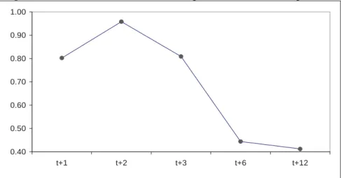
In general, we obtain the lowest MAPE values for longer forecasting horizons (6 and 12 months). These results confirm previous research by Teräsvirta et al. (2005), who obtain more accurate forecasts with ANN models at long forecast horizons, and are indicative that SVRs and ANNs are particularly suitable for medium and long term forecasting. In Figure 2 we graph the evolution of the mean of the MAPE statistic for all models and regions for the different forecasting horizons. It can be seen how the overall forecasting performance improves for longer forecast horizons.
Figure 2. Mean MAPE for all models and regions for each forecasting horizon
0.40 0.50 0.60 0.70 0.80 0.90 1.00 t+1 t+2 t+3 t+6 t+12
Source: Compiled by the author.
When analyzing the results by regions, we obtain the highest MAPE values for the Balearic Islands. This result can somehow be explained by the high levels of dispersion in tourist arrivals to the Balearic Islands (Table 1a). Nevertheless, when increasing the memory values, we find a higher relative improvement in the Balearic islands than in the rest of the regions for all models. This result indicates that the number of previous observations used for concatenation has a different effect on the forecasting
performance for different regions. The best forecasting results are usually obtained in Andalucia, Castilla La Mancha, Extremadura and Murcia.
Table 3a. Forecast accuracy. MAPE (2013:03-2014:01)
Support Vector Regressions Artificial Neural Networks Linear kernel Polynomial
kernel Gaussian RBF kernel RBF MLP SVR_1 SVR_2 SVR_3 ANN_1 ANN_2 Andalucia 1 month 0.376 0.516 0.373 0.374 0.384 2 months 0.425 0.311 0.486 0.396 0.412 3 months 0.379 0.398 0.439 0.398 0.365 6 months 0.287 0.375 0.323 0.364 0.317 12 months 0.145 0.265 0.144* 0.250 0.186 Aragon 1 month 0.424 0.370 0.370 0.342 0.345 2 months 0.463 0.478 0.393 0.368 0.405 3 months 0.363 0.299 0.266 0.351 0.385 6 months 0.318 0.337 0.309 0.307 0.258* 12 months 0.311 0.353 0.306 0.306 0.273 Asturias 1 month 0.902 0.983 0.872 0.714 0.678 2 months 1.057 0.961 0.851 0.734 0.840 3 months 0.613 0.424 0.454 0.656 0.705 6 months 0.428 0.590 0.375 0.440 0.384 12 months 0.295* 0.427 0.312 0.434 0.350 Balearic Islands 1 month 5.705 8.474 6.440 4.031 3.753 2 months 7.231 9.756 6.562 5.066 5.148 3 months 4.609 3.173 4.713 5.019 4.669 6 months 1.004 2.419 0.943* 2.587 1.178 12 months 1.510 2.682 1.424 2.241 1.454 Canary Islands 1 month 0.471 0.547 0.456 0.420 0.420 2 months 0.439 0.458 0.420 0.414 0.414 3 months 0.449 0.469 0.444 0.416 0.426 6 months 0.413 0.430 0.415 0.412 0.411* 12 months 0.476 0.531 0.473 0.414 0.431 Cantabria 1 month 1.206 1.477 1.109 0.899 1.103 2 months 1.308 1.612 1.007 0.874 0.984 3 months 0.896 0.499 0.403 0.854 0.851 6 months 0.364 0.597 0.249* 0.434 0.344 12 months 0.311 0.448 0.323 0.483 0.315 Castilla y Leon 1 month 0.635 0.731 0.632 0.544 0.518 2 months 0.701 0.772 0.638 0.562 0.606 3 months 0.561 0.294 0.503 0.542 0.540 6 months 0.281 0.416 0.220 0.342 0.230 12 months 0.192 0.364 0.188* 0.286 0.243 Castilla La Mancha 1 month 0.324 0.356 0.343 0.264 0.265 2 months 0.332 0.369 0.294 0.280 0.301 3 months 0.297 0.431 0.256 0.289 0.288 6 months 0.218 0.258 0.182 0.213 0.183 12 months 0.092 0.183 0.075* 0.157 0.127 Catalonia 1 month 0.450 0.511 0.446 0.416 0.427 2 months 0.562 0.558 0.486 0.438 0.483 3 months 0.442 0.312 0.332 0.410 0.410 6 months 0.382 0.370 0.397 0.341 0.331 12 months 0.335 0.344 0.329 0.328 0.291*
Table 3b. Forecast accuracy. MAPE (2013:03-2014:01)
Support Vector Regressions Artificial Neural Networks Linear kernel Polynomial
kernel Gaussian RBF kernel RBF MLP SVR_1 SVR_2 SVR_3 ANN_1 ANN_2 Valencia 1 month 0.328 0.478 0.335 0.341 0.309 2 months 0.396 0.371 0.401 0.359 0.363 3 months 0.363 0.315 0.363 0.362 0.363 6 months 0.362 0.221* 0.357 0.357 0.357 12 months 0.309 0.508 0.297 0.317 0.276 Extremadura 1 month 0.333 0.344 0.339 0.346 0.332 2 months 0.380 0.361 0.368 0.355 0.354 3 months 0.328 0.397 0.461 0.351 0.319 6 months 0.316 0.365 0.277 0.332 0.306 12 months 0.212 0.311 0.196* 0.270 0.212 Galicia 1 month 0.929 1.066 0.902 0.731 0.732 2 months 1.054 1.130 0.648 0.795 0.860 3 months 0.705 0.483 0.593 0.751 0.776 6 months 0.491 0.638 0.388 0.537 0.423 12 months 0.357 0.842 0.355 0.453 0.356 Madrid (Community) 1 month 0.261 0.344 0.255 0.291 0.258 2 months 0.283 0.318 0.273 0.283 0.256 3 months 0.296 0.183* 0.299 0.285 0.268 6 months 0.297 0.288 0.296 0.288 0.269 12 months 0.233 0.440 0.240 0.281 0.256 Murcia(Region) 1 month 0.250 0.251 0.244 0.238 0.243 2 months 0.301 0.287 0.263 0.265 0.289 3 months 0.260 0.229 0.251 0.282 0.297 6 months 0.249 0.210 0.250 0.276 0.291 12 months 0.211 0.279 0.197 0.201 0.180* Navarra 1 month 0.682 0.779 0.660 0.590 0.587 2 months 0.766 0.917 0.704 0.604 0.665 3 months 0.597 0.499 0.522 0.565 0.573 6 months 0.418 0.548 0.339 0.452 0.365 12 months 0.331 0.469 0.328* 0.396 0.351 Basque Country 1 month 0.444 0.457 0.432 0.432 0.495 2 months 0.529 0.493 0.466 0.440 0.483 3 months 0.429 0.387 0.378 0.420 0.430 6 months 0.420 0.355* 0.459 0.387 0.386 12 months 0.388 0.436 0.380 0.411 0.381 La Rioja 1 month 0.586 0.662 0.527 0.499 0.501 2 months 0.642 0.395 0.408 0.544 0.581 3 months 0.598 0.454 0.347 0.553 0.543 6 months 0.367 0.482 0.255 0.338 0.278 12 months 0.202 0.349 0.181* 0.337 0.227 Total 1 month 0.431 0.530 0.388 0.369 0.382 2 months 0.468 0.574 0.447 0.391 0.417 3 months 0.383 0.271 0.330 0.370 0.355 6 months 0.313 0.322 0.305 0.295 0.254 12 months 0.261 0.326 0.241* 0.265 0.279
In order to attain a more comprehensive forecasting evaluation, we also compute the percentage of Periods with Lower Absolute Error (PLAE) statistic proposed by Claveria, Monte and Torra (2016). The PLAE is a dimensionless measure based on the CJ
statistic for testing market efficiency (Cowles and Jones, 1937). This accuracy measure allows us to compare the forecasting performance between two competing models (Table 4a and 4b).
The statistic consists on a ratio that calculates the proportion of periods in which the model under evaluation obtains a lower absolute forecasting error than the benchmark model. In this study we use the no-change model as a benchmark. Let us denote yt as actual value and yˆt as forecast at period t 1,,n. Forecast errors can then be defined as et yt yˆt. Given two competing models A and B, where A refers to the
forecasting model under evaluation and B stands for benchmark model, we can then obtain the proposed statistic as follows:
n Ȝ PLAE n t t ¦ 1 where °¯ ° ® otherwise 0 if 1 t,A t,B t e e Ȝ (12)
Finally, we repeat the experiment assuming different topologies regarding the
memory values. These values represent the number of lags introduced when running the models, denoting the number of previous months used for concatenation. The number of lags used in the different experiments ranged from one to three months for all the
models. Results of the forecasting competition expanding the memory up to three lags are shown in Tables 5a and 5b and Tables 6a and 6b.
When the forecasts are obtained incorporating additional lags of the time series (Table 5a, 5b, 6a and 6b), we obtain better forecasting results in most cases. Unlike Claveria, Monte and Torra (2014), who did not obtained significant differences when additional lags are incorporated in the feature vector, we find that increasing the
dimensionality of the input may help improve the forecast accuracy of SVRs and ANNs. The reason for this discrepancy can be due to the length of the time series used in the analysis, as longer time series favour the learning process of the models.
Table 4a. Forecast accuracy. PLAE (2013:03-2014:01)
Support Vector Regressions Artificial Neural Networks Linear kernel Polynomial
kernel Gaussian RBF kernel RBF MLP SVR_1 SVR_2 SVR_3 ANN_1 ANN_2 Andalucia 1 month 27.3 9.1 36.4 18.2 18.2 2 months 54.5 45.5 54.5 45.5 45.5 3 months 63.6 63.6 63.6 54.5 63.6 6 months 72.7 72.7 72.7 72.7 81.8 12 months 18.2 9.1 18.2 0.0 9.1 Aragon 1 month 18.2 36.4 9.1 36.4 27.3 2 months 36.4 45.5 45.5 45.5 45.5 3 months 63.6 81.8 81.8 63.6 63.6 6 months 81.8 72.7 72.7 81.8 100.0 12 months 18.2 27.3 18.2 36.4 27.3 Asturias 1 month 18.2 9.1 18.2 27.3 18.2 2 months 36.4 45.5 63.6 54.5 45.5 3 months 72.7 81.8 81.8 72.7 72.7 6 months 100.0 90.9 81.8 100.0 90.9 12 months 0.0 0.0 0.0 9.1 0.0 Balearic Islands 1 month 27.3 27.3 45.5 36.4 27.3 2 months 54.5 45.5 54.5 54.5 54.5 3 months 72.7 72.7 63.6 72.7 72.7 6 months 100.0 100.0 100.0 100.0 100.0 12 months 18.2 0.0 18.2 0.0 9.1 Canary Islands 1 month 0.0 0.0 0.0 0.0 9.1 2 months 9.1 9.1 9.1 9.1 9.1 3 months 9.1 0.0 9.1 9.1 9.1 6 months 0.0 0.0 0.0 0.0 0.0 12 months 0.0 0.0 0.0 0.0 0.0 Cantabria 1 month 18.2 18.2 36.4 36.4 18.2 2 months 54.5 36.4 63.6 54.5 54.5 3 months 72.7 72.7 72.7 63.6 63.6 6 months 90.9 100.0 90.9 100.0 90.9 12 months 9.1 0.0 9.1 9.1 27.3 Castilla y Leon 1 month 36.4 27.3 36.4 36.4 36.4 2 months 45.5 45.5 63.6 54.5 54.5 3 months 54.5 63.6 72.7 63.6 63.6 6 months 81.8 90.9 90.9 81.8 90.9 12 months 0.0 9.1 0.0 9.1 9.1 Castilla La Mancha 1 month 36.4 36.4 36.4 45.5 54.5 2 months 54.5 54.5 54.5 63.6 63.6 3 months 72.7 63.6 72.7 63.6 63.6 6 months 81.8 81.8 81.8 81.8 81.8 12 months 45.5 36.4 63.6 45.5 36.4 Catalonia 1 month 18.2 27.3 18.2 18.2 18.2 2 months 36.4 36.4 45.5 45.5 45.5 3 months 63.6 63.6 72.7 63.6 54.5 6 months 81.8 63.6 81.8 81.8 81.8 12 months 0.0 0.0 0.0 18.2 18.2
Notes: Percentage of PLAE values in parentheses. The PLAE ratio measures the number of out-of-sample periods with lower absolute errors than the benchmark model (No-change model).
Table 4b. Forecast accuracy. PLAE (2013:03-2014:01)
Support Vector Regressions Artificial Neural Networks Linear kernel Polynomial
kernel Gaussian RBF kernel RBF MLP SVR_1 SVR_2 SVR_3 ANN_1 ANN_2 Valencia 1 month 9.1 18.2 9.1 27.3 18.2 2 months 36.4 36.4 36.4 45.5 36.4 3 months 54.5 54.5 54.5 54.5 54.5 6 months 63.6 81.8 63.6 63.6 63.6 12 months 0.0 0.0 0.0 9.1 9.1 Extremadura 1 month 36.4 27.3 27.3 27.3 36.4 2 months 54.5 45.5 45.5 45.5 45.5 3 months 54.5 54.5 54.5 54.5 54.5 6 months 72.7 63.6 72.7 63.6 72.7 12 months 27.3 18.2 27.3 9.1 9.1 Galicia 1 month 18.2 9.1 27.3 27.3 27.3 2 months 45.5 45.5 63.6 54.5 54.5 3 months 63.6 90.9 54.5 63.6 63.6 6 months 81.8 90.9 81.8 81.8 90.9 12 months 0.0 0.0 0.0 9.1 9.1 Madrid (Community) 1 month 27.3 9.1 27.3 18.2 27.3 2 months 36.4 27.3 36.4 36.4 36.4 3 months 18.2 54.5 18.2 27.3 27.3 6 months 36.4 45.5 36.4 45.5 36.4 12 months 0.0 0.0 0.0 0.0 0.0 Murcia(Region) 1 month 27.3 45.5 27.3 18.2 27.3 2 months 27.3 27.3 27.3 27.3 27.3 3 months 54.5 54.5 54.5 54.5 45.5 6 months 72.7 72.7 72.7 72.7 72.7 12 months 27.3 18.2 18.2 27.3 27.3 Navarra 1 month 9.1 9.1 9.1 27.3 27.3 2 months 45.5 36.4 45.5 45.5 45.5 3 months 72.7 72.7 72.7 72.7 72.7 6 months 81.8 81.8 81.8 81.8 90.9 12 months 9.1 18.2 18.2 0.0 18.2 Basque Country 1 month 27.3 27.3 27.3 9.1 18.2 2 months 27.3 36.4 27.3 45.5 36.4 3 months 63.6 63.6 63.6 63.6 63.6 6 months 72.7 72.7 72.7 72.7 72.7 12 months 0.0 0.0 0.0 0.0 0.0 La Rioja 1 month 36.4 18.2 36.4 45.5 36.4 2 months 63.6 63.6 63.6 63.6 63.6 3 months 63.6 72.7 63.6 72.7 63.6 6 months 81.8 81.8 81.8 81.8 81.8 12 months 18.2 27.3 18.2 9.1 27.3 Total 1 month 9.1 0.0 9.1 18.2 27.3 2 months 45.5 45.5 54.5 45.5 45.5 3 months 63.6 63.6 63.6 54.5 63.6 6 months 81.8 81.8 81.8 81.8 90.9 12 months 0.0 0.0 0.0 18.2 9.1
Notes: Percentage of PLAE values in parentheses. The PLAE ratio measures the number of out-of-sample periods with lower absolute errors than the benchmark model (No-change model).
Table 5a. Forecast accuracy. MAPE (2013:03-2014:01) – Expanded memory up to three lags Support Vector Regressions Artificial Neural Networks Linear kernel Polynomial
kernel Gaussian RBF kernel RBF MLP SVR_1 SVR_2 SVR_3 ANN_1 ANN_2 Andalucia 1 month 0.255 0.303 0.273 0.386 0.301 2 months 0.343 0.359 0.331 0.396 0.314 3 months 0.400 0.391 0.441 0.387 0.443 6 months 0.267 0.345 0.222 0.389 0.333 12 months 0.143 0.213 0.132* 0.356 0.141 Aragon 1 month 0.441 0.492 0.377 0.354 0.317 2 months 0.403 0.433 0.353 0.348 0.350 3 months 0.363 0.289 0.266* 0.342 0.325 6 months 0.320 0.347 0.356 0.350 0.294 12 months 0.304 0.297 0.303 0.350 0.339 Asturias 1 month 0.678 0.736 0.551 0.647 0.604 2 months 0.687 0.682 0.587 0.678 0.672 3 months 0.476 0.751 0.434 0.652 0.557 6 months 0.418 0.760 0.301 0.587 0.378 12 months 0.305 0.363 0.292 0.585 0.287* Balearic Islands 1 month 3.271 9.987 5.016 4.821 4.852 2 months 4.594 12.723 5.906 5.024 3.736 3 months 3.874 3.804 3.913 4.401 4.530 6 months 1.698 2.796 1.519 3.749 1.079 12 months 1.436 2.611 1.457 3.643 0.980* Canary Islands 1 month 0.478 0.564 0.464 0.396 0.429 2 months 0.455 0.647 0.406 0.401 0.449 3 months 0.452 0.525 0.437 0.400 0.459 6 months 0.430 0.468 0.419 0.400 0.406 12 months 0.458 0.499 0.441 0.394* 0.457 Cantabria 1 month 0.902 1.127 0.558 0.822 0.599 2 months 0.854 1.296 0.779 0.823 0.958 3 months 0.625 0.953 0.806 0.783 0.805 6 months 0.362 0.603 0.220* 0.678 0.233 12 months 0.348 0.496 0.346 0.698 0.275 Castilla y Leon 1 month 0.484 0.554 0.343 0.524 0.495 2 months 0.447 0.505 0.337 0.510 0.414 3 months 0.399 0.277 0.274 0.489 0.411 6 months 0.291 0.374 0.173 0.453 0.221 12 months 0.191 0.324 0.178 0.484 0.165* Castilla La Mancha 1 month 0.248 0.300 0.213 0.277 0.269 2 months 0.272 0.288 0.174 0.286 0.234 3 months 0.204 0.160 0.132 0.290 0.193 6 months 0.210 0.225 0.207 0.253 0.250 12 months 0.097 0.164 0.088 0.236 0.084* Catalonia 1 month 0.346 0.382 0.364 0.420 0.333 2 months 0.365 0.405 0.373 0.405 0.398 3 months 0.356 0.342 0.291* 0.400 0.362 6 months 0.375 0.343 0.349 0.383 0.367 12 months 0.323 0.392 0.331 0.374 0.357
Table 5b. Forecast accuracy. MAPE (2013:03-2014:01) – Expanded memory up to three lags Support Vector Regressions Artificial Neural Networks Linear kernel Polynomial
kernel Gaussian RBF kernel RBF MLP SVR_1 SVR_2 SVR_3 ANN_1 ANN_2 Valencia 1 month 0.301 0.343 0.300 0.353 0.299 2 months 0.311 0.339 0.365 0.359 0.349 3 months 0.325 0.192* 0.461 0.359 0.412 6 months 0.364 0.338 0.253 0.354 0.347 12 months 0.295 0.506 0.287 0.349 0.232 Extremadura 1 month 0.284 0.309 0.254 0.350 0.295 2 months 0.303 0.406 0.322 0.344 0.284 3 months 0.296 0.283 0.304 0.351 0.290 6 months 0.285 0.349 0.335 0.346 0.311 12 months 0.204 0.337 0.197* 0.339 0.205 Galicia 1 month 0.759 0.960 0.636 0.727 0.662 2 months 0.844 0.944 0.723 0.732 0.714 3 months 0.727 0.633 0.487 0.711 0.755 6 months 0.469 0.665 0.403 0.628 0.358 12 months 0.362 0.585 0.357 0.659 0.347* Madrid (Community) 1 month 0.274 0.327 0.261 0.288 0.242 2 months 0.261 0.312 0.292 0.287 0.269 3 months 0.299 0.287 0.280 0.288 0.296 6 months 0.291 0.236 0.204 0.291 0.251 12 months 0.224 0.360 0.212 0.276 0.195* Murcia(Region) 1 month 0.246 0.307 0.230 0.262 0.229 2 months 0.272 0.283 0.263 0.262 0.262 3 months 0.251 0.266 0.256 0.265 0.321 6 months 0.243 0.218 0.230 0.257 0.326 12 months 0.198 0.213 0.198 0.245 0.165* Navarra 1 month 0.564 0.617 0.555 0.550 0.440 2 months 0.540 0.625 0.416 0.558 0.525 3 months 0.416 0.615 0.375 0.534 0.468 6 months 0.367 0.513 0.345 0.512 0.413 12 months 0.338* 0.456 0.343 0.514 0.348 Basque Country 1 month 0.382 0.407 0.433 0.421 0.409 2 months 0.375 0.374 0.334 0.421 0.424 3 months 0.378 0.395 0.325* 0.410 0.375 6 months 0.443 0.448 0.351 0.395 0.372 12 months 0.389 0.454 0.374 0.395 0.432 La Rioja 1 month 0.528 0.952 0.405 0.548 0.547 2 months 0.578 0.739 0.370 0.549 0.468 3 months 0.367 0.817 0.340 0.541 0.405 6 months 0.319 0.382 0.222 0.466 0.280 12 months 0.196 0.277 0.169* 0.527 0.226 Total 1 month 0.315 0.396 0.301 0.366 0.302 2 months 0.332 0.441 0.399 0.361 0.267 3 months 0.298 0.359 0.434 0.359 0.275 6 months 0.321 0.402 0.220* 0.335 0.293 12 months 0.255 0.258 0.255 0.328 0.267
Table 6a. Forecast accuracy. PLAE (2013:03-2014:01) – Expanded memory up to three lags Support Vector Regressions Artificial Neural Networks Linear kernel Polynomial
kernel Gaussian RBF kernel RBF MLP SVR_1 SVR_2 SVR_3 ANN_1 ANN_2 Andalucia 1 month 45.5 63.6 36.4 27.3 0.0 2 months 63.6 63.6 54.5 36.4 54.5 3 months 54.5 54.5 54.5 45.5 45.5 6 months 81.8 72.7 81.8 72.7 90.9 12 months 18.2 0.0 18.2 0.0 9.1 Aragon 1 month 9.1 36.4 63.6 45.5 0.0 2 months 63.6 45.5 54.5 45.5 45.5 3 months 72.7 72.7 81.8 63.6 63.6 6 months 81.8 72.7 72.7 72.7 81.8 12 months 18.2 36.4 18.2 18.2 18.2 Asturias 1 month 45.5 27.3 63.6 18.2 0.0 2 months 63.6 54.5 72.7 54.5 63.6 3 months 81.8 81.8 81.8 72.7 81.8 6 months 90.9 100.0 90.9 90.9 90.9 12 months 9.1 9.1 9.1 9.1 9.1 Balearic Islands 1 month 45.5 36.4 63.6 36.4 0.0 2 months 45.5 36.4 45.5 54.5 54.5 3 months 72.7 72.7 90.9 72.7 72.7 6 months 100.0 100.0 100.0 100.0 100.0 12 months 18.2 9.1 18.2 18.2 0.0 Canary Islands 1 month 0.0 0.0 63.6 81.8 0.0 2 months 9.1 0.0 9.1 9.1 9.1 3 months 9.1 0.0 9.1 0.0 0.0 6 months 0.0 0.0 0.0 0.0 0.0 12 months 0.0 0.0 0.0 0.0 0.0 Cantabria 1 month 36.4 36.4 63.6 45.5 0.0 2 months 54.5 45.5 63.6 63.6 54.5 3 months 81.8 72.7 81.8 72.7 72.7 6 months 90.9 81.8 100.0 100.0 100.0 12 months 9.1 18.2 18.2 0.0 9.1 Castilla y Leon 1 month 45.5 36.4 54.5 18.2 0.0 2 months 63.6 54.5 81.8 54.5 63.6 3 months 72.7 72.7 72.7 63.6 72.7 6 months 81.8 81.8 90.9 81.8 90.9 12 months 0.0 9.1 0.0 0.0 0.0 Castilla La Mancha 1 month 27.3 45.5 72.7 36.4 0.0 2 months 54.5 54.5 90.9 54.5 63.6 3 months 72.7 63.6 72.7 72.7 72.7 6 months 90.9 90.9 90.9 100.0 81.8 12 months 45.5 45.5 36.4 36.4 72.7 Catalonia 1 month 27.3 27.3 63.6 27.3 0.0 2 months 63.6 54.5 63.6 45.5 54.5 3 months 72.7 72.7 72.7 54.5 63.6 6 months 81.8 81.8 81.8 72.7 81.8 12 months 0.0 0.0 0.0 0.0 0.0
Notes: Percentage of PLAE values in parentheses. The PLAE ratio measures the number of out-of-sample periods with lower absolute errors than the benchmark model (No-change model).
Table 6b. Forecast accuracy. PLAE (2013:03-2014:01) – Expanded memory up to three lags Support Vector Regressions Artificial Neural Networks Linear kernel Polynomial
kernel Gaussian RBF kernel RBF MLP SVR_1 SVR_2 SVR_3 ANN_1 ANN_2 Valencia 1 month 18.2 54.5 54.5 36.4 0.0 2 months 45.5 45.5 54.5 45.5 45.5 3 months 54.5 81.8 54.5 54.5 45.5 6 months 63.6 63.6 72.7 63.6 72.7 12 months 0.0 0.0 0.0 0.0 27.3 Extremadura 1 month 36.4 36.4 45.5 45.5 0.0 2 months 72.7 54.5 54.5 45.5 63.6 3 months 54.5 54.5 54.5 54.5 45.5 6 months 72.7 72.7 81.8 63.6 90.9 12 months 27.3 0.0 18.2 0.0 18.2 Galicia 1 month 27.3 36.4 45.5 45.5 0.0 2 months 63.6 54.5 63.6 54.5 63.6 3 months 72.7 72.7 72.7 63.6 63.6 6 months 81.8 81.8 81.8 81.8 90.9 12 months 0.0 0.0 0.0 0.0 0.0 Madrid (Community) 1 month 18.2 27.3 54.5 36.4 0.0 2 months 36.4 18.2 27.3 27.3 27.3 3 months 27.3 27.3 18.2 18.2 18.2 6 months 36.4 54.5 54.5 36.4 45.5 12 months 0.0 0.0 0.0 0.0 0.0 Murcia(Region) 1 month 18.2 36.4 45.5 63.6 0.0 2 months 27.3 27.3 27.3 36.4 27.3 3 months 63.6 54.5 54.5 54.5 45.5 6 months 81.8 81.8 72.7 72.7 72.7 12 months 18.2 27.3 9.1 27.3 27.3 Navarra 1 month 18.2 27.3 54.5 36.4 0.0 2 months 63.6 63.6 72.7 54.5 54.5 3 months 81.8 72.7 81.8 72.7 81.8 6 months 81.8 81.8 81.8 81.8 81.8 12 months 0.0 0.0 9.1 9.1 9.1 Basque Country 1 month 36.4 54.5 72.7 45.5 0.0 2 months 45.5 54.5 54.5 54.5 36.4 3 months 63.6 63.6 63.6 63.6 54.5 6 months 72.7 63.6 81.8 63.6 72.7 12 months 0.0 9.1 0.0 0.0 0.0 La Rioja 1 month 36.4 63.6 72.7 45.5 0.0 2 months 63.6 63.6 63.6 54.5 54.5 3 months 72.7 63.6 72.7 72.7 63.6 6 months 81.8 81.8 81.8 81.8 81.8 12 months 27.3 18.2 27.3 0.0 27.3 Total 1 month 9.1 18.2 45.5 27.3 0.0 2 months 63.6 54.5 54.5 36.4 72.7 3 months 72.7 72.7 72.7 63.6 81.8 6 months 81.8 81.8 90.9 81.8 81.8 12 months 0.0 18.2 0.0 0.0 9.1
Notes: Percentage of PLAE values in parentheses. The PLAE ratio measures the number of out-of-sample periods with lower absolute errors than the benchmark model (No-change model).
The PLAE with regard to the no-change model (Table 4a and 4b and Table 6a and 6b), shows that the SVR_3 and ANN_1 are the models that outperform the no-change model in most cases for 2, 3 and 6 months-ahead forecasts. There is ample evidence in the literature that the no-change model generates more accurate one-period-ahead predictions than other more sophisticated models (Witt, Witt and Wilson, 1994). The only exceptions are the Canary Islands and the Community of Madrid, where no model outperforms the no-change model. This result can be explained by the fact that they are the only regions that do not show strong seasonal patterns.
These results confirm previous research by Hong (2006) and Chen and Wang (2007), who obtain better forecasting results with SVMs and SVRs than with ANNs for tourist arrivals to Barbados and China respectively. Velásquez et al. (2010) also obtain better predictions with SVMs than with MLP ANNs. Nevertheless, not all SVRs show the same performance. While SVRs with a Gaussian RBF kernel outperform ANNs in most cases, MLP ANNs outperform both SVRs with linear and polynomial kernels.
The fact that the Gaussian RBF kernel is easier to implement and especially suitable for non-linear data sets, suggests the potential of SVRs for non-linear time series forecasting. These results also show the importance of properly selecting the kind of kernel function.
7. Summary and Conclusions
As more accurate predictions are essential for effective policy planning, new forecasting methods provide room for improvement. Artificial intelligence techniques based on statistical learning such as Support Vector Regressions and Artificial Neural Networks have attracted increasing interest to refine the predictions. From the wide array of techniques, we have focused on the SVRs based on three different kernels and two ANN architectures that represent alternative ways of handling information.
The main purpose of this study is to assess the forecasting accuracy of Support Vector Machines. First, we compare the forecasting accuracy of three different SVR models to two ANNs. We then compare all models with respect to a benchmark by means of a dimensionless forecasting accuracy measure based on the statistic for testing market efficiency. This statistic allows comparing the forecasting performance between two competing models by giving the percentage of periods in which the model under
evaluation obtains a lower absolute forecasting error than the benchmark model. Finally, we repeat the experiment increasing the number of lags used for concatenation in order to analyze what is the effect of the memory on the forecasting results.
The forecasting out-of-sample comparison shows that the SVR with a Gaussian RBF kernel outperforms the rest of the models in most cases. When comparing the
forecasting accuracy of the different techniques, we find that MLP networks show a better forecasting performance than RBF ANNs and linear and polynomial SVRs. This result illustrates the importance of not overlooking the parameter and kernel function selection for SVR modelling.
When analyzing the differences between regions, we obtain the best forecasting results in Castilla La Mancha. On the other hand, the Balearic Islands display the highest forecasting errors. This result can partly be explained by the fact that tourist arrivals to the Balearic Islands show high levels of dispersion.
Regarding the forecasting horizons, we obtain the best results for six and twelve months ahead forecasts, suggesting the suitability of SVRs and ANNs for mid and long term forecasting.
When repeating the experiment for topologies with a higher number of lags, we find that MLP ANNs relatively improve their forecasting performance. Apart from this result, we find no major differences in the forecasting accuracy when additional lags are incorporated in the feature vector. The fact that increasing the dimensionality of the input does not have a significant effect on forecast accuracy is indicative that the increase in the weight matrix is not compensated by the more complex specification, leading to overparametrization.
This study contributes to the forecasting literature and to the tourism industry by highlighting the suitability of applying SVR with Gaussian RBF kernels for estimating future demand. The comparison of this novel statistical learning method to alternative artificial intelligence techniques such as the Gaussian process regression is a question to be addressed in further research. Another question to be considered is whether the combination of the forecasts of different statistical learning statistical learning techniques may improve the forecasting performance of practical tourism demand forecasting.
Acknowledgements
This work was supported by the Ministerio de Economía y Competitividad under the SpeechTech4All Grant (TEC2012-38939-C03-02).
References
Aguiló, E., and J. Rosselló (2005). “Host Community Percepti