Online Resource Allocation with Structured Diversification

Online Resource Allocation with Structured Diversification

Nicholas Johnson

Arindam Banerjee

Abstract

A variety of modern data analysis problems, ranging from finance to job scheduling, can be considered as online resource allocation (ORA) problems. A key consideration in such ORA problems is some notion of risk, and suitable ways to alleviate risk. In several settings, the risk is structured so that groups of assets, such as stocks, are exposed to similar risks. In this paper, we present a formulation for online resource allocation with structured diversification (ORASD) as a constrained online convex optimization problem. The key novel component of our formulation is a constraint on the L(∞,1) group norm of the resource allocation vector, which ensures that no single group gets a large share of the resource and, unlike L(1,p) norms used for overlapping group Lasso, does not impose sparsity structures over groups. We instantiate the problem in the context of portfolio selection, propose an efficient ADMM algorithm, and illustrate the effectiveness of the formulation through extensive experiments on two benchmark datasets.

1 Introduction

A variety of modern data analysis problems can be con-sidered as resource allocation problems. The problems range from investment of resources to a variety of assets, such as investing money in the stock market or assign-ing teams to software projects, to modern systems level challenges, such as job scheduling in compute clusters or data/content storage and delivery over the internet. Increasingly, such problems need to be solved dynam-ically and repeatedly in response to external changes, e.g., movements in the stock market, new jobs for com-pute servers, changes in demand for data/content, etc.

A key consideration in such online resource alloca-tion (ORA) problems is some noalloca-tion of risk, and suitable ways to diversify the allocation to alleviate risk. For portfolio selection, putting all of ones money in one or a few stocks is considered risky, since those few stocks may not perform well over time. Further, companies usually invest in multiple projects, rather than one or a ∗_{Department of Computer Science and}

Engineer-ing, University of Minnesota, Minneapolis, MN 55455

{njohnson,banerjee}@cs.umn.edu

few, since some of those projects will succeed and sev-eral others may fail. One considers similar notions of risk and diversification strategies for systems level chal-lenges, such as fault-tolerant designs for compute job scheduling and provisioning for data/content delivery.

In several such ORA settings, the risk is often struc-tured and calls for strucstruc-tured diversification strategies. For example, in portfolio selection, one considers mar-ket sectors, such as energy, technology, utilities, etc., which gives a structure beyond individual stocks. Of-ten, stocks within a sector move together in response to external influences so that investing in just one sec-tor can be risky. A structurally diverse portfolio would invest in multiple sectors to alleviate risk.

In this paper, we present a novel formulation for on-line resource allocation with structured diversification (ORASD). The formulation considers groups over the assets of interest, such as stocks, where the groups can be of different sizes and they can overlap. We also out-line a way in which these groups can be inferred from the data, e.g., based on their correlation structures. The key novel component of our formulation is the L(∞,1) group norm, which is rather different from L(1,p) type group norms typically used for overlapping group Lasso and related problems. We pose the ORASD problem as a suitable online convex optimization problem with the constraint that the L(∞,1) group norm of the resource allocation vector has to be bounded within a prespeci-fied limit. Such a constraint ensures that no single group gets a large share of the resource. Further, unlike over-lapping group Lasso, there is no sparsity restriction on the resource allocation vector, so that one can invest in all assets if that helps the resource allocation objective. We instantiate the problem in the context of portfolio selection and propose an efficient algorithm based on the alternating direction method of multipliers (ADMM). We illustrate the effectiveness through extensive experi-ments on two benchmark datasets and several baselines from the existing literature.

We arrange the rest of the paper as follows. In Section 2 we discuss related work. In Section 3 we introduce our formulation. In Section 4 we instantiate the formulation to portfolio selection, and discuss the algorithm. In Section 5 we discuss the experimental results and we conclude in Section 6.

2 Related Work

There is a large literature on resource allocation with many papers posing the problem as an auction [11], mechanism design problem [2], Markov Decision Pro-cess [12, 24], matching problem [15], and planning prob-lem [16, 27]. However, few have considered risk when computing allocations in an online fashion [14, 18, 19]. Additionally, little work in online portfolio selection have considered risk in their algorithmic setting [8]. However, previous work [1, 5, 6, 7, 9, 10, 17] have shown that their algorithms are guaranteed to perform compet-itively with certain families of adaptive portfolios even in an adversarial market in a costless setting without making any statistical assumptions regarding the move-ment of the stocks.

3 Diversified Resource Allocation

In this section, we introduce a framework for resource al-location with structured diversity, and consider the on-line resource allocation problem under such structured diversity. In Section 4, we consider the online portfo-lio selection problem as an instance of such diversified resource allocation.

3.1 Structured Diversity with L(∞,1) Norm We consider a resource allocation problem over n objects, where the goal is find a probability distributionp∈∆n, the n-dimensional probability simplex, which deter-mines how to split up a resource over thenobjects such that a certain (convex) objective f(p) is minimized. For example, in the context of investment (portfolio se-lection), the n objects can be different assets (such as stocks), andpis an investment strategy, i.e., what frac-tion of one’s resources (say, money) should one put on each asset (stock). The basic idea of diversification is to avoid putting all of the resources on one asset. A simple way to accomplish this is to put a cap or upper bound on the amount of resources which can be put on any asset, i.e., p(i) ≤κ for some κ∈ [0,1]. A poten-tial issue with such an approach is that there may be structural dependencies between the assets. For exam-ple, in the context of portfolio selection, selling some Google stocks to buy Apple stocks may not accomplish the goals of diversification when the entire tech sector goes down. In this example, Google and Apple as assets can be considered structurally related, both being part of the tech sector. The goal of structured diversification is to develop diversification strategies which explicitly consider such structurally related groups and diversify across such groups.

For the development, we assume knowledge of such structurally related groups, and outline approaches for inferring such groups directly from the data in

Section 4 in the context of portfolio selection. Let

G ={g1, . . . , gm} be the set of groups, where gi is the set of indices for theni assets in the group. The groups can be of different sizes, |gi|=ni, and the groups may overlap, i.e., gi∩gj6=∅.

Given such group structure, we introduce theL(∞,1) group norm which plays a key role in structured diver-sity. For anyx∈Rn and a set of (possibly overlapping, different sized) groups G, theL(∞,1)group norm is de-fined as: kxkG_(∞,1)= kxg1k1. . .kxgmk1 > _∞ (3.1)

where xgi is a vector of lengthnwith value equal tox

for indices in gi and 0 otherwise. The L(∞,1) group norm is determined by the largest L1 norm over all groups in G. This norm is rather different in character compared to the L(1,2) norm [21], used in the context of overlapping group Lasso and multi-task learning, as well as the L(1,∞) group norm [23]. The L(1,p) group norms accomplish sparsity over the groups, i.e., certain groups can become all zeroes. Such a structure is not desirable in the context of diversified portfolio selection, since one wants to distribute the resource to multiple groups for diversification. In fact, forkxkG

(∞,1)≤κ, each individual groupgihas the flexibility of increasing their

L1norm toκwithout changing the norm ball (penalty). Similarly, one could also consider any L(∞,p) group norm, which looks at the maximum overLpnorms over groups. In the context of resource allocation, since the key object of interest is a probability distribution, we work with the L(∞,1) group norm in this paper. Thus, for the purposes of structured diversity in resource allocation, we will consider problems of the form

min p∈∆n

f(p) s.t. kpkG_(∞,1)≤κ ,

(3.2)

for a suitably chosen κ∈[0,1].

3.2 Online Resource Allocation Several resource allocation problems need to be solved online, i.e., dy-namically over time. Such a problem can be modeled as an online optimization problem with objective function

ft(p) at timet. In such an online setting, the optimiza-tion proceeds in rounds where in round tthe algorithm has to pick a solution from a feasible set,pt∈∆n, with-out knowingft(·) and incur a loss offt(pt). In addition to being feasible, we add two additional requirements on pt: (1) pt needs to stay close topt−1 since we do not want the resource allocation to change drastically in every time step, which may have a cost associated with it, and (2)kptkG_(∞,1)≤κso that structural diversity is maintained over time. Thus, the sub-problem at timet

takes the form (3.3) min

p∈∆n

η `t(p) + Ω(p,pt−1) s.t.kpkG<sub>(∞,1)</sub>≤κ , where`tdenotes a suitable resource allocation loss and Ω(·,·) is a convex penalty function based on the change in pt. Ideally, over T rounds we would like to minimize the constrained cumulative loss

(3.4) T

X

t=1

η `t(pt) + Ω(pt,pt−1) s.t.kptkG_(∞,1)≤κ .

However, in the online setting, absolute minimization of (3.4) is not feasible since we do not know the sequence of `t a priori. Alternatively, over T rounds we intend to get a sequence ofptsuch that the followingregret is sub-linear in T, i.e., RT = T X t=1 ft(pt)−min p∗ T X t=1 ft(p∗)≤o(T) (3.5)

where ft(p)=η`t(p)+Ω(p,pt−1). The regret is mea-suredw.r.t the best fixed minimizer in hindsightp∗.

Following recent advances in online convex opti-mization, in order to accomplish a sub-linear regret, in each step (t+1), we consider solving a linearized version of the problem obtained by a first-order Taylor expan-sion offt atptalong with a proximal term, so that

pt+1= argmin p∈∆n kpkG (∞,1)≤κ ηhp,∇`t(pt)i+d(p,pt), (3.6)

where d(p,pt) = 1₂kp −ptk22 + λΩ(p,pt) and the parameters η, λ ≥ 0. As we discuss in Section 4, one can extend existing arguments to obtain a sub-linear regret bound for such online resource allocation.

4 Diversified Online Portfolio Selection

Given the resource allocation with structured diversity framework, we now introduce online portfolio selection and propose a primal-dual algorithm for solving (3.6) in this context.

4.1 Online Portfolio Selection We consider a stock market consisting of n stocks{s1, . . . , sn} over a span of T periods. For ease of exposition, we will con-sider a period to be a day, but the analysis presented holds for any valid definition of a ‘period’ such as an hour or a month. Let xt(i) denote the price relativeof stocksi in dayt, i.e., the multiplicative factor by which the price ofsichanges in dayt. Hence,xt(i)>1 implies a gain, xt(i) <1 implies a loss, and xt(i) = 1 implies the price remained unchanged. We assume, xt(i) > 0

∀ i, t. Let xt= [xt(1), . . . , xt(n)]> denote the vector of price relatives for day t, and let x1:t denote the collec-tion of such price relative vectors up to and including day t. A portfolio pt = [pt(1), . . . , pt(n)]> ∈ ∆n on day t can be viewed as a probability distribution over

n stocks that prescribes investingpt(i) fraction of the current wealth in stock si. Note that the portfolio pt has to be decided before knowing xt which will be re-vealed only at the end of the day. The multiplicative gain in wealth at the end of day t is then p>

t xt. For a sequence of price relatives x1:t−1={x1, . . . ,xt−1}up to day (t−1), the sequential portfolio selection problem in day t is to determine a portfolio pt based on past performance of the stocks. At the end of dayt,xtis re-vealed and the actual performance ofptgets determined by p>_txt. Over T periods, for a sequence of portfolios

p1:T ={p1, . . . ,pT}, the multiplicative gain in wealth is ST(p1:T,x1:T) = Q

T

t=1 p>txt and the logarithmic gain in wealth isLST(p1:T,x1:T) =P T t=1log p > txt . Ideally, for a costless environment (no transaction costs) we would like to maximize LST(p1:T,x1:T) over

p1:T. However, online portfolio selection cannot be posed as a batch optimization problem due to the temporal nature of the choices: xt is not available when one has to decide on pt. Further, (statistical) assumptions regarding xtcan be difficult to make.

4.2 ORASD Algorithm Online portfolio selection can now be viewed as a special case of our online re-source allocation with structured diversity setting where

`t(pt) = −log(p>t xt), and Ω = kp−ptk1. The L1 penalty term on the difference of two consecutive port-folios measures the fraction of wealth traded and encour-ages lazy updates to the portfolio to limit transaction costs. The parameter λ controls the amount that can be traded every day. The L(∞,1) penalty term forces the portfolio to spread out the investment amongst the groups. The level of diversification depends on the value of κ. Additionally, since we allow overlapping groups and will solve (3.6) via lifting, we need to add a con-sensus constraint pgi =Sgip ∀i where pgi is a vector

of length n with value equal to pfor indices in gi and 0 otherwise and Sgi is a known diagonal matrix with

Sgi(j, j) = 1 if elementjis in groupgiand 0 otherwise.

The online portfolio selection with structured diversifi-cation problem is now

min p∈∆n kpkG (∞,1)≤κ S_gip=p_gi∀i ηhp,∇`t(pt)i+1 2kp−ptk 2 2+λkp−ptk1 . (4.7)

Algorithm 1ORASD Algorithm with ADMM 1: Inputpt,xt,Sg1,...,gm, η, λ, β 2: Initializep,pgi,z,ui,v∈0 n_{, k= 0} 3: Set ˆa= ((1 +β)I+β(Sg1+· · ·+Sgm)) −1 4: ADMM iterations pk+1=Y ∆n ˆ a ηxt p>t xt +ˆa(1+β)pt+ˆaβ Sg1(p k g1−u k 1)+. . .+ (4.9) Sgm(p k gm−u k m)+zk−vk ! pkgi+1= Y k·k1≤κ Sgip k+1_+uk i ∀i (4.10) zk+1=Sλ/β(pk+1−pt+vk) (4.11) uk_i+1=uki+Sgip k+1_−pk+1 gi ∀i (4.12) vk+1=vk+pk+1−pt−zk+1 (4.13) where Q

∆n is the projection to the simplex andSρ is the shrinkage operator.

5: Continue untilStopping Criteriais satisfied

objective withL(∞,1)and linear constraints. We can use ADMM to solve this problem by introducing auxiliary variablez=p−ptand moving the inequality constraint into the objective function if we leth(pgi) =1(kpgik1≤κ)

where kpkG (∞,1)≤κ≡ kpgik1≤κ∀i min p∈∆n S_gip=p_gi∀i p−pt=z ηhp,∇`t(pt)i+1 2kp−ptk 2 2+λkzk1+ m X i=1 h(pgi). (4.8)

The ADMM formulation in (4.8) naturally lets us decouple the non-smooth terms from the smooth terms, which is computationally advantageous. The augmented Lagrangian for (4.8) is

L(p,pg1...gm,z,u1...m,v) = (4.14) ηhp,∇`t(pt)i+ 1 2kp−ptk 2 2+λkzk1+ m X i=1 h(pgi) +β 2 m X i=1 kSgip−pgi+uik 2 2+ β 2kp−pt−z+vk 2 2

where u and v are scaled dual variables. ADMM consists of the following iterations

pk+1:= argmin p∈∆n ηhp,∇`t(pt)i+1 2kp−ptk 2 2 (4.15) +β 2 m X i=1 kSgip−p k gi+u k ik 2 2+ β 2kp−pt−z k_+vk k22

Algorithm 2Diversified Online Portfolio Selection

1: Inputη, λ, β; Transaction costγ, Days lagnumlag

2: Initializep0(i) =_n1 i= 1, . . . , n, S γ 0 = $1

3: Fort= 1, . . . , T

4: Receivext, the vector of price relatives

5: Compute wealth: S_tγ=S_tγ₋₁pT txt−γkpt−pt−1k1 6: Ift≤numlag 7: pt+1(i) =_n1 i= 1, . . . , n(uniform portfolio) 8: Else 9: Compute groups: G 10: Update: pt+1=ORASD(pt,xt,G, η, λ, β) 11: end for pk_g+1_i := argmin p_gi h(pgi)+ β 2kSgip k+1_−p gi+u k ik 2 2∀i (4.16) zk+1:= argmin z λkzk1+ β 2kp k+1 −pt−z+vkk22 (4.17) uk_i+1:=uki +Sgip k+1_−pk+1 gi ∀i (4.18) vk+1:=vk+pk+1−pt−zk+1 . (4.19)

p-update: We solve for p be taking the gradient of (4.15)w.r.t. pand setting it to zero to get the closed form update ofpas p=Y ∆n ˆ a ηxt p>_txt +ˆa(1+β)pt+ˆaβSg1(p k g1−u k 1)+. . .+ (4.20) Sgm(p k gm−u k m)+z k_−vk where ˆa= ((1 +β)I+β(Sg1+· · ·+Sgm)) −1 andQ ∆n

is a projection to the probability simplex as in [13].

pgi-updates: We solve for each pgi in parallel by

projecting to theL1 ball of radiusκas in [13]

pgi= Y k·k1≤κ Sgip k+1 +uki . (4.21)

z-update: We solve forzby using the soft-thresholding operator Sρ(a) [20]

z=Sλ/β(pk+1−pt+vk). (4.22)

ui-updates: The ui-updates are already in closed form and can be computed in parallel for all i.

v-updates: Thev-update is already in closed form. Algorithm 1 shows the complete ADMM based algorithm with the closed form updates. The stopping criteria for the ORASD algorithm is based on the primal and dual residuals from [4]. Algorithm 2 is our diversified online portfolio selection algorithm. It uses

the ORASD algorithm to compute pt+1. It takes in an additional parameter γ which is a fixed percentage charged for the total amount of transaction every day.

S_tγ is the transaction cost-adjusted cumulative wealth gain at the end oftdays.

4.3 Regret Bound We sequentially invest with the diverse portfoliosp1,· · ·,pT obtained from Algorithm 2 and on daytsuffer a lossft(pt) =η`t+λkpt−pt−1k1, where `t =−log(p>txt). Our goal is to minimize the

regret with respect to the best fixed portfolio p∗ in hindsight. We establish the standard regret bound in portfolio selection literature [1, 6, 17] and follow [9] closely with minor modifications.

Theorem 1 Let p∗ ∈ P be the fixed portfolio obtained from min p PT t=1`t(p). For η= √ T andk∇`t(pt)k ≤G, the regret can be bounded as,

(4.23) η T X t=1 `t(pt)+λ T X t=2 kpt−pt−1k1−η T X t=1 `t(p∗)≤O( √ T),

where `tis a strongly convex function and the sequence

pt and the fixed optimal portfolio p∗ all lie in P :=

{p|p∈∆n,kpkG(∞,1)≤κ}. 5 Experiments and Results

5.1 Datasets The experiments were conducted on data taken from the New York Stock Exchange (NYSE) and the Standard & Poor’s 500 (S&P 500) stock market index. The NYSE dataset [6] consists of 36 stocks with data accumulated over a period of 22 years from July 3, 1962 to December 31, 1984 and has been widely used in the literature [1, 3, 6, 17]. The S&P500 dataset [7] consists of 263 stocks which were present in the S&P500 index in 2010 and were alive since 1990.

5.2 Methodology and Parameter Setting In all our experiments we start with $1 as our initial invest-ment and an initial portfolio which is uniformly dis-tributed over all the stocks. We use Algorithm 2 to ob-tain our portfolios sequentially and compute the trans-action cost-adjusted wealth each day.

For our experiments, we utilize the follow method for computing the groups. For the previous numlag days, we compute the correlation graph C over the stocks. To compute structurally related groups, we set a correlation threshold on the edges of the graph and if an edge has weight < then it is removed resulting in C. For each stock in C, we construct a group around it by including its neighbors withinkhops away. For example, if k = 1 then we construct group gi

by including stock si and only its directly connected neighbors in the group. As such, there will be exactly

n groups but the size of each group may vary. For our experiments, we allow the groups to change each day.

Since the two datasets are very different in na-ture (stock composition and duration), we experimented with various parameter values. We found stable behav-ior across the following range of parameters: numlag ∈

{5,10,15}, ={0.90,0.95}, and β = 2. Additionally, we experimented extensively with a large range of values forηandλfrom 10−6_{to 10}3_{and values forκfrom 0.1 to} 1.0 to observe their effect on our portfolio. Moreover, we chose a reasonable range of γ values between 0% and 2% to compute the proportional transaction costs incurred due to the portfolio update every day. We have illustrated some of our results with representative plots from either the NYSE or S&P500 dataset.

We use the wealth obtained from OLU [9], EG [17], a uniform constant rebalanced portfolio (U-CRP), and a buy-and-hold strategy as benchmarks for our exper-iments. For U-CRP, we make trades to rebalance the portfolio at the end of each day after the market move-ment has driven it away from the uniform distribution. For the buy-and-hold case we start with a uniformly dis-tributed portfolio and do a hold on the positions there-after, i.e., no trades. We do not consider algorithms such as Anticor [3] or OLMAR [22], which are good heuristics but without regret bounds.

5.3 Effect of the L(∞,1) group norm and κ The

L(∞,1) group norm encourages diversity between the groups and sparsity within the groups. This structure is further effected by the value of κ which has direct control over the level of diversity. κhas an effect on (a) the value of kptkG_(∞,1) each day, (b) the group weight

kpgik1∀i, and (c) the number of active groups.

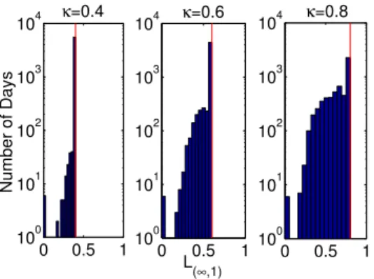
(a) Value of kptkG_(∞,1) With the diversity inducing constraint kptkG_(∞,1) ≤ κ we are encouraging different levels of diversity depending on the value of κ. From Figure 1, we can see the effect κhas onkptkG_(∞,1)with

η = 100 and λ = 10−6_{. With a low κ value of 0.4,}

kptkG_(∞,1) is small with many days seeing the value exactly equal to κ. As we increase κ, we see that the value moves along with κ with many days seeing the value equal κ. This behavior is consistent with aggressive trading due to the high η and low λvalues. ORASD tries to invest as much wealth as allowed into groups that performed well in the past. With higher λ

this behavior is not as aggressive and the value more slowly moves with κand becomes more spread out.

0 0.5 1 100 101 102 103 104 Number of Days κ=0.4 0 0.5 1 100 101 102 103 104 L₍ ∞,1) κ=0.6 0 0.5 1 100 101 102 103 104 κ=0.8

Figure 1: Total value ofkptkG(∞,1)with vertical red lines marking the value of κ. With an aggressive trading strategy, the value closely follows the increasingκ.

(b) Group Weight kpgik1 Not only is the value of kptkG_(∞,1) affected by κ, but so are the group weights

kpgik1∀i. Each of these are constrained to be less than

or equal to κ and how close each group’s weight gets to κ is of interest. If there are many days which see many groups with weight close to κand many groups with little weight then this suggests ORASD is focusing on a few groups to invest the majority of wealth in at each day. If, however, there are many days with small group weight and few with large this suggests ORASD is investing a small amount of wealth in many groups and has a more diversified portfolio.

From Figure 2 we can see with η = 10−3 _and

λ= 10−6 _{ORASD utilizes a more conservative trading} strategy. We can see this from how slowly the distri-bution moves with κ and from how many days see a small amount of wealth invested in each group. With low η and λ, ORASD does not trade aggressively and is further limited byκ. The portfolio is diversified with smallκand becomes slightly less so as we increaseκ.

(c) Number of Active Groups We define an active group as a group which has a significant percent of wealth invested in it. The number of active groups can be a measure of how diverse a portfolio is. If there are many active groups this implies a diverse portfolio where few active groups does not. From Figure 3 we can see that for lowκ= 0.1, the number of active groups is reasonably high with around 20 groups active out of 263 (about 8%). With low κ we are forcing a diverse portfolio therefore many groups have a significant amount of wealth invested in them. For high κ= 0.9, we see that the number of active groups drops to around 3 groups (about 1%). This implies that ORASD is focusing on a handful of well performing groups. This trading strategy has a potentially high

0 0.5 1 100 101 102 103 104 105 Number of Days κ=0.4 0 0.5 1 100 101 102 103 104 105

Total Group Weight

κ=0.6 0 0.5 1 100 101 102 103 104 105 κ=0.8

Figure 2: Total group weightkpgik1∀iwith vertical red

lines marking the value of κ. With lowκwe are forced to diversify but less so asκincreases.

reward but it also carries high risk. We can see how adjusting the value ofκcan provide us the flexibility to use drastically different trading strategies.

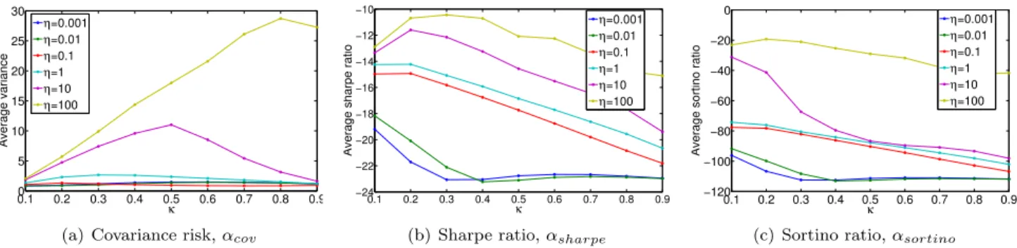
5.4 Risk andκ Even though our online resource al-location with structured diversification framework (3.6) does not explicitly take risk into account, we can effec-tively control risk using κas a proxy. We observe how the value of κ affects the amount of risk our diverse online portfolio is exposed to using three common measures of risk: (a) covariance, (b) Sharpe ratio, and (c) Sortino ratio.

(a) Covariance We compute the covariance Σtusing the previous numlag days of price relatives. We mea-sure the risk of a portfolioptw.r.t. a uniform constant rebalanced portfolio uas αcov=p>tΣtpt/u>Σtu. High

αcov implies high risk and lowαcov implies low risk.

(b) Sharpe ratio The Sharpe ratio [25] measures

‘91 ‘93 ‘95 ‘97 ‘99 ‘01 ‘03 ‘05 ‘07 ‘09 0 50 κ=0.1 ‘91 ‘93 ‘95 ‘97 ‘99 ‘01 ‘03 ‘05 ‘07 ‘09 0 50 κ=0.9

Number of Active Groups

Figure 3: Number of active groups for the S&P500 dataset. For low κwe trade with a more conservative, diversified portfolio while with high κ we are more aggressive and risk seeking.

0.10 0.2 0.3 0.4 0.5 0.6 0.7 0.8 0.9 5 10 15 20 25 30 κ Average variance η=0.001 η=0.01 η=0.1 η=1 η=10 η=100

(a) Covariance risk,αcov

0.1 0.2 0.3 0.4 0.5 0.6 0.7 0.8 0.9 −24 −22 −20 −18 −16 −14 −12 −10 κ

Average sharpe ratio

η=0.001 η=0.01 η=0.1 η=1 η=10 η=100

(b) Sharpe ratio,αsharpe

0.1 0.2 0.3 0.4 0.5 0.6 0.7 0.8 0.9 −120 −100 −80 −60 −40 −20 0 κ

Average sortino ratio

η=0.001 η=0.01 η=0.1 η=1 η=10 η=100

(c) Sortino ratio,αsortino

Figure 4: For αcov with lowη, the risk stays low for varyingκ. For large η, the risk increases with an increasing

κ. For both αsharpe andαsortino, the risk-adjusted return is higher for higher η and deceases as we increaseκ. From this figure, we can see that if we want to control the risk exposure, we can effectively do it by controllingκ.

how much the return (percent gain or loss on in-vestment) of a portfolio compensates for the level of risk taken. It computes what can be considered as a risk-adjusted return for a given portfolio and benchmark return. It does this by measuring both the downwards and upwards volatility. A higher Sharpe ratio implies better compensation for the risk expo-sure. We compute the Sharpe ratio of a portfolio as

αsharpe=(R−Rb)/

p

var(R−Rb) where R is the return for the portfolio andRb is the benchmark return which is typically a large index such as the S&P500.

(c) Sortino ratio The Sortino ratio [26] is similar to the Sharpe ratio however it only measures the downwards volatility. Typically, upwards volatility is encouraged as we would gladly accept the price of a stock we have invested in to go up. However, the Sharpe ratio penalizes this type of volatility where the Sortino ratio does not. We compute the Sortino ratio as αsortino = (R−Rb)/DR whereDR is the standard deviation of negative returns (losses).

From Figure 4, we can see the behavior of the three measures of risk for varying values of η and κ with

λ= 10−6_{. Forα}

cov in 4(a), with low values ofηthe risk is low and stays low as we increaseκ. However, once we have higherη values, the risk starts to increase up to a point before it starts to show a decreasing trend as we increaseκ. With higherη, the portfolio is focusing more on maximizing returns and is only investing in stocks that performed well in the past. This behavior does afford the portfolio the ability to earn huge amounts of wealth, however, as we can see it also exposes the investor to huge amounts of risk. In 4(b) and 4(c), we see that the risk-adjusted return increases as we increase

η however, the curve trends downwards as we increase

κ. This again implies that as κ increases so does the risk. From these plots we can see thatκis a good proxy

to risk and we can therefore control risk by setting κ.

5.5 Transaction Cost-Adjusted Wealth To eval-uate the practical application of ORASD we analyze the performance by calculating the transaction cost-adjusted cumulative wealth. We do this for varying val-ues ofκto get a sense of the tradeoff between risk and return. We compare the performance of ORASD to the state-of-the-art algorithms OLU, EG, U-CRP, buy-and-hold, and the best stock in hindsight (without transac-tion costs) with empirically determined parameters.

From Figure 5 we can see that for optimal η and

λvalues and varying values ofκ, ORASD returns more wealth than all the other competing algorithms for the NYSE dataset. ORASD earns $163.07 compared to $54.14 for the single best stock (Morris), $50.80 for OLU, $27.08 for U-CRP, $26.70 for EG, and $14.50 for buy-and-hold. ORASD returns over 3x as much as OLU and the best single stock we could have chosen

0.1 0.15 0.2 0.25 0.3 0.35 0.4 0.45 0.5 0 50 100 150 200 κ Wealth No transaction cost γ=1e−06 γ=5e−06 γ=1e−05 γ=5e−05 γ=0.0001 Buy−and−hold U−CRP EG

Best Stock (Morris) OLU

Figure 5: Transaction cost-adjusted wealth for the NYSE dataset. ORASD returns more wealth than competing algorithms even with transaction costs.

0.1 0.2 0.3 0.4 0.5 0.6 0.7 0.8 0.9 0 1 2 3 4 Average Entropy κ NYSE S&P500

(a) Entropy of ORASD for η=100, λ=10−6_{. High entropy}

implies the investment is more spread out. As κ increases, the entropy decreases which implies that the portfolio is concentrated on a single group of stocks.

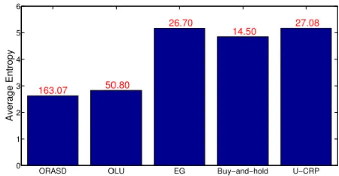
ORASD OLU EG Buy−and−hold U−CRP

0 1 2 3 4 5 6 163.07 50.80 26.70 14.50 27.08 Average Entropy

(b) Entropy of ORASD and competing algorithms with cumu-lative wealth. ORASD has around the same level of diversifi-cation as OLU but returns more wealth.

Figure 6: Average entropy for ORASD and competing algorithms. We can see that as κ decreases so does the entropy. This indicates that the portfolio is becoming less diverse and as such may be exposed to more risk.

in hindsight. We can see that ORASD also returns more wealth than the competing algorithms even with transaction costs.

5.6 Diversification We saw from Figure 3 that one way to measure the diversity of a portfolio is by the number of active groups. Another measure commonly used is the entropy of the portfolio. Entropy measures how spread out a distribution is. If we have a portfolio with high entropy this implies that the portfolio is invested in many groups and is more diversified where with low entropy the portfolio only has investments in a few groups and is not as diversified.

From Figure 6(a), we can see that as κ increases the entropy decreases. This shows that with highκthe portfolio is focusing on a few groups to invest in and

Covariance −Sharpe −Sortino

0 20 40 60 80 100 120 Risk Value ORASD OLU EG Buy−and−hold U−CRP

Figure 7: Risk comparison between competing algo-rithms for the NYSE dataset. We plot the negative Sharpe and Sortino ratios therefore the higher the bar the higher the risk.

as such may be exposed to more risk. This again gives evidence thatκcan be used as a proxy to risk.

Finally, we want to compare how diversified ORASD is against competing algorithms. We can see from Figure 6(b) that ORASD has the lowest entropy but is close to that of OLU. However, ORASD returns more than 3x as much wealth as OLU for the same level of diversity and risk exposure.

5.7 Risk Comparison From Section 5.5, we saw that ORASD is able to return more wealth than all of the state-of-the-art algorithms. However, as Markowitz postulated, we should seek low risk in addition to high returns. As such, we compare the risk exposure for each of the competing algorithms with optimal parameters with respect to wealth. To be consistent in the plot and have each bar represent the level of risk exposure, we have plotted the negative Sharpe and Sortino ratios since a low ratio implies a high risk relative to the return. Therefore, for each of the bar plots, a higher bar height implies higher risk.

In Figure 7 we can see that ORASD has lowerαcov than OLU but higher than the others with κ = 0.2, however, the other algorithms returned far less wealth. There is a balance between risk taken and potential returns. Forαsharpe, we can see that ORASD and OLU are reasonably close and both have smaller risk than the other algorithms. For αsortino, ORASD has the smallest risk. This can be explained by the fact that both the Sharpe and Sortino ratios compute the risk-adjusted return and the competing algorithms do not return much wealth so the compensation for the risk is low.

6 Conclusion

In this paper, we have developed an online resource allocation with structured diversification framework and an online learning algorithm (ORASD) and showed how it can be applied to the problem of online portfolio selection. Our analysis shows that ORASD is competitive with reasonable fixed strategies which have the power of hindsight. Our experimental results illustrate the effect of the diversity inducing group normL(∞,1)on the diversification of the portfolio, risk exposure, and wealth. We show that ORASD is able to outperform the state-of-the-art online portfolio se-lection algorithms in terms of wealth earned even with reasonable transaction costs and risk exposure. In the future we wish to explore extending our framework to allow long and short positions as well as meta portfolios.

Acknowledgements

The research was supported in part by NSF grants IIS-1447566, IIS-1422557, CCF-1451986, CNS-1314560, IIS-0953274, IIS-1029711, and by NASA grant NNX12AQ39A. AB also acknowledges support from IBM and Yahoo. The authors would also like to thank Maria Gini for her helpful feedback.

References

[1] A. Agarwal, E. Hazan, S. Kale, and R. Schapire. Algorithms for portfolio management based on the newton method. InICML, pages 9–16, 2006.

[2] Maria-Florina Balcan and Avrim Blum. Mechanism design via machine learning. InFOCS, pages 605–614, Washington, DC, USA, 2005. IEEE Computer Society. [3] A. Borodin, R. El-Yaniv, and V. Gogan. Can we learn

to beat the best stock. JAIR, 21:579–594, 2004. [4] S. Boyd, N. Parikh, E. Chu, B. Peleato, and J.

Eck-stein. Distributed optimization and statistical learn-ing via the alternatlearn-ing direction method of multipliers.

Foundations and Trends in Machine Learning, 3(1):1– 122, 2011.

[5] N. Cesa-Bianchi and G. Lugosi. Prediction, Learning, and Games. Cambridge University Press, 2006. [6] T. Cover. Universal portfolios.Mathematical Finance,

1:1–29, 1991.

[7] P. Das and A. Banerjee. Meta optimization and its application to portfolio selection. InKDD, 2011. [8] Puja Das and Arindam Banerjee. Online quadratically

constrained convex optimization with applications to risk adjusted portfolio selection. Technical report, Department of Computer Science and Engineering, University of Minnesota, 2012.

[9] Puja Das, Nicholas Johnson, and Arindam Banerjee. Online lazy updates for portfolio selection with trans-action costs. InAAAI, pages 202–208, 2013.

[10] Puja Das, Nicholas Johnson, and Arindam Banerjee. Online portfolio selection with group sparsity. In

AAAI, pages 1185–1191, 2014.

[11] Nikhil R. Devanur and Thomas P. Hayes. The adwords problem: Online keyword matching with budgeted bidders under random permutations. InEC, pages 71– 78, New York, NY, USA, 2009. ACM.

[12] Dmitri A. Dolgov and Edmund H. Durfee. Resource al-location among agents with mdp-induced preferences.

JAIR, pages 27–505, 2006.

[13] J. Duchi, Y. Singer, and T. Chandra. Efficient projec-tions onto the l1-ball for learning in high dimensions. InICML, 2008.

[14] Stefano Ermon, Jon Conrad, Carla Gomes, and Bart Selman. Risk-sensitive policies for sustainable renew-able resource allocation. InIJCAI, pages 1942–1948. AAAI Press, 2011.

[15] Gagan Goel and Aranyak Mehta. Online budgeted matching in random input models with applications to adwords. In SODA, pages 982–991, Philadelphia, PA, USA, 2008. Society for Industrial and Applied Mathematics.

[16] Daniel Golovin, Andreas Krause, Beth Gardner, Sarah J. Converse, and Steve Morey. Dynamic resource allocation in conservation planning. InAAAI, 2011. [17] D. Helmbold, E. Schapire, Y. Singer, and M. Warmuth.

On-line portfolio selection using multiplicative weights.

Mathematical Finance, 8(4):325–347, 1998.

[18] J. W. Horwood. Risk-sensitive optimal harvesting and control of biological populations. Mathematical Medicine and Biology, 13(1):35–71, 1996.

[19] Ronald A. Howard and James E. Matheson. Risk-sensitive markov decision processes. Management Sci-ence, 18(7):pp. 356–369, 1972.

[20] R. Jenatton, J. Mairal, G. Obozinski, and F. Bach. Proximal methods for hierarchical sparse coding.

JMLR, pages 2297–2334, 2010.

[21] R. Jenatton, J. Mairal, G. Obozinski, and F. Bach. Proximal methods for sparse hierarchical dictionary learning. InICML, 2010.

[22] B. Li and S. Hoi. On-line portfolio selection with moving average reversion. InICML, 2012.

[23] Julien Mairal, Rodolphe Jenatton, Francis R. Bach, and Guillaume R. Obozinski. Network flow algorithms for structured sparsity. In NIPS, pages 1558–1566. 2010.

[24] Remi Munos. Efficient resources allocation for markov decision processes. InNIPS, pages 1571–1578, 2001. [25] William Sharpe. Mutual fund performance.Journal of

Business, pages 119–138, 1966.

[26] Frank Sortino and R van der Meer. Downside risk.

Journal of Portfolio Management, pages 27–31, 1991. [27] Shan Xue, Alan Fern, and Daniel Sheldon. Dynamic

resource allocation for optimizing population diffusion. InAISTATS, pages 1033–1041, 2014.