Does Mortgage Hedging Raise Long-Term Interest Rate Volatility? *

Preliminary Draft: Please do not quote without the authors' permission.

Does Mortgage Hedging Raise Long-Term Interest Rate Volatility?

*

by

Yan Chang, Douglas McManus and Buchi Ramagopal

Freddie Mac

Office of the Chief Economist

8200 Jones Branch Drive

McLean, VA 22102

July 2004

* _{The authors are grateful to Frank Nothaft, Ed Golding, and Peter Zorn for their suggestions and insights. We} would like to thank Jorge Reis, Mitch Post and Jim Berkovec for their comments. Bob Winata helped with the construction of the data set and thanks to Murat Karakurt for his insights into swaptions volatility. The views presented are those of the authors and not of Freddie Mac. We are responsible for the remaining errors.

2

Abstract

Does Mortgage Hedging Raise Long-Term Interest Rate Volatility?

This paper examines the impact of mortgage hedging activities on interest rate volatility. A recent analysis by Perli and Sack (2003) provides a framework for evaluating this question and along with estimates of the extent to which hedging by agents in the mortgage market amplifies interest rate volatility. We evaluate the amplification issue by considering a wider range of interest rate derivatives and implementing different measures of hedging intensity to isolate the sources that might be contributing to volatility. By considering a rolling window over which we obtain maximum likelihood estimates of key parameters we show that the extent to which mortgage hedging determines volatility is driven completely by two episodes: the collapse of LTCM and the market reaction in the aftermath of the 9/11 tragedy. We conclude that it is difficult to make the case that hedging by mortgage market participants is responsible for exacerbating volatility.

3

1. Introduction

Volatility is an ever-present feature of financial markets. Recent history has evidenced several episodes of heightened volatility. Events such as the Russian debt crisis, the collapse of LTCM, and the disruption of the Asian markets in the late 1990’s have all been responsible for periods of heightened volatility. While such volatility can be viewed from a macroeconomic perspective as the source of economic instability, from a complete markets perspective, this volatility represents the efficient functioning of markets in the face of uncertainty. Over the past two decades,

markets, institutions, and practices have been examined as possible sources of ‘excessive’ volatility. This paper examines the possible role of mortgage hedging in creating volatility in interest rate markets.

Starting in 1990, 30-year fixed mortgage rates declined from a high of 10.5% to a low of 5.2% in June of 2003. This decline in rates led households to refinance their mortgages in record

numbers. The refinancing activity peaked during the years of 1992-1993, 1998 and most recently, in 2003. By the end of 2003, up to 40-45% of the $7.0 trillion single-family debt outstanding was financed, in 2003 alone. The volume of refinancing activity in 2003, for example, led to more than three trillion dollars of mortgage debt outstanding to be re-struck at lower rates. Despite the huge volume, the US mortgage market managed to respond flexibly, providing homeowners the benefit of lower rates.

The decline in rates and the re-striking of mortgage debt has led an increasing number of

mortgage market participants such as originators, mortgage-servicers, and portfolio managers to manage the risks associated with this secular decline in rates. Since fixed rate mortgages have positive duration and negative convexity, market participants can choose a mixture of static and dynamic hedging strategies to mitigate the associated interest rate risk. Static hedging of

mortgage interest rate risk can be accomplished by issuing callable debt or through the synthesis of callable debt engineered by the purchase of swaptions. Dynamic hedging, on the other hand, calls for the constant management of the relative durations of the assets and liabilities, typically through swap transactions. Counterparties to these derivative transactions have diversified books of business and can consequently manage these risks. However, they also serve as

intermediaries in the market for these transactions by identifying others parties that might naturally offset these mortgage market risks.

The nature and magnitude of mortgage hedging activities has raised the issue of its impact on market interest rates. Several approaches have been taken to this problem. Naranjo and Toevs (2002) suggest that large mortgage market participants reduce volatility in mortgage rates as a result of their participation in the market. Alternatively, another characterization by Perli and Sack (2003) suggests that mortgage hedging raises long-term rate volatility. The argument of Perli and Sack suggests that the tools of financial engineering, as applied to mortgage risk management might be responsible for heightened volatility. This paper investigates this claim. The issue of whether rational speculators or risk management frameworks can destabilize prices or exacerbate volatility has been a subject of continued research. One position, starting with Friedman (1953) is that rational speculators act to stabilize asset prices. In Friedman’s view “Speculators who destabilized prices by, on average, buying when prices were high and selling when they were low would find this unsustainable and be eliminated from the market. The more

4

rational speculators who moved prices back toward fundamentals would eliminate such speculators, who are less than rational and moved prices away from fundamentals.”

Alternatively, several recent researchers have developed theoretical examples in which trading activities can destabilize prices. In these examples, rational speculators might not easily stabilize asset prices even when they have access to identical information, and have identical priors as shown by Hart and Kreps (1986). Similarly, DeLong, Schleifer, Summers and Waldmann (1990) also show, for example, that investors with extrapolative expectations, those who chase trends, or have stop-loss orders in place, all of which could be characterized as positive feedback investment strategies, might contribute to destabilizing market movements.

Arguments similar to those of destabilizing speculation have been used to make the case that risk management in general, or portfolio insurance in particular, contributes to greater volatility in rates or asset prices. Portfolio insurance, for example, according to the Brady Report, was considered to have been the exacerbating factor in the crash of 1987.

In a similar vein, the Value-at Risk (VaR) methodology has also been blamed for amplifying volatility (See Persaud (2000) and Dunbar (2000)). The argument is that shocks might raise volatility initially, leading to a breach of VaR positions and require investors to raise the amount of allocated capital; otherwise investors would be required to liquidate some part of their

portfolios. It further raises the possibility that large institutions that exceed predetermined VaR measures (determined internally by management or, externally by a regulator) might then simultaneously “sell the same asset at the same time, creating higher volatility and correlations,

which amplify the initial effect, forcing additional sales.”1 However, Jorion (2002) claims that

such criticisms relating to the VaR framework have been misplaced.

In effect, the argument presented by Perli and Sack is that when rates rise, mortgage hedgers sell off Treasuries either directly or synthetically through swaps further amplifying the increase in rates. Conversely, in response to declining rates mortgage hedgers will purchase long duration assets, amplifying the decline in rates. The magnitude of the amplification effects will depend on the degree to which mortgage hedgers adopt dynamic rather than static hedging strategies. Underlying their argument is the assumption that some constant proportion of mortgage interest rate risk is actively managed through dynamic rather than static hedging strategies.

While the arguments presented by Perli and Sack are appealing, their “amplification proposition” i.e., mortgage hedging amplifies rate movements, is similar to arguments that have been made in different settings. A recent line of argument that has been proposed, with the implication of eliminating the need to delta hedge, is to push for the adoption of adjustable rate mortgages. While it would eliminate the need on the part of large mortgage holders to delta hedge, it ignores the possible impact on individual homeowners and the fact that they may not be in a position to efficiently manage such interest rate risk as evidenced by higher ARM default rates for otherwise

identical mortgages.

It is in fact ironic that ARMs are being proposed as an alternative to fixed rate mortgages in the US market at a point when countries such as the UK see the prevalence of ARMs as being one of the reasons for their boom-bust housing cycles, which increases the amplitude of their business

1 _{Jorion (2002)}

5

cycles. The review of the housing market in the UK by David Miles (2004) highlights the need for the UK housing market to introduce longer term mortgages with prepayment options, much like those in the US mortgage market.

Still, the question remains as to whether or not delta hedging by mortgage market participants creates volatility, and if so, the extent to which this is the case. Ultimately, the issue of impact of mortgage hedging and the impact on volatility is one that has to be determined empirically. In the interest of consistency, we use a framework identical to that of Perli and Sack and lay out the framework in section 2. The data along with results of the first stage regression are described in section 3. The results of the first part of the empirical exercise, measuring the extent to which mortgage hedging exacerbates volatility is presented in section 4. The final arguments and summary of results are presented in the conclusion.

2. The Model

The underlying intuition of the framework utilized is that changes in the long-term rates are driven by a data generating process. The shocks generated by this process emanate from monetary policy innovations, news and changes in risk preferences. The long-term rate in question is the ten-year swap rate and changes in this rate between time t and t+n are generated

by a “fundamental” shock ε(t,t+n). The changes in the ten-year swap rate are characterized as:

(

t,t n

)

(t,t n)

r + = _t ∗ +

∆ γ ε (1)

In this setting, the fundamental shock ε(t,t+n) is exacerbated by a factor γ_t , whose value is

known at time “t” and whose magnitude is determined by the degree of mortgage hedging

activity. This amplification factor is supposed to characterize the state of the mortgage market at the beginning of the period. It takes on a value that could be close to one if the extent of

prepayment risk is low, and values that are higher values if prepayment risk is greater. Thus shocks, during periods of high prepayment risk are amplified and shocks during periods of low prepayment risk are dampened.

Using the specification in (1), the variance of the interest rate is characterized as:

2 , 2 ,t t t r γ σε σ_∆ = . (2)

The expression describes the second moment of the ten-year swap rate as a function of the second moment of the fundamental shock and the amplification factor. The conditional variance of the fundamental shocks is described as following an AR(1) process:

t t t = 0 + 1 2,−1+u 2 , ε ε α α σ σ . (3)

Using equation (2) to rewrite last period’s fundamental variance as ratio of last period’s variance of the swap rate to the amplification factor and using (3), equation (2) is expressed as:

6 t t t r t t t t r _γ σ γ u γ α γ α σ = + _{∆ −} + − ∆ 2, 1 1 1 0 2 , (4)

During periods of higher prepayment risk when γ is higher it raises the average level of

volatility, the first term on the right hand side of (4), will be higher. The second term above highlights the autocorrelation of volatility, and third term describes the “volatility of volatility” effect. This term describes the fact that , as Perli and Sack point out, shows that changes in expected volatility are greater when prepayment risk is high.

The framework for determining the magnitude of the amplification factor γ_t , is described as:

t t βX

γ =1+ , (5)

where Xt is a measure of hedging intensity. When there is no hedging pressure the value of γ_tis

one, and higher when there is an increased need for greater mortgage market hedging. Various proxies of mortgage market hedging needs are considered and we discuss them further in the next section which discusses data.

Using the specification for the hedging amplification factor in (5), (4) can be rewritten as

t t t r t t t t r _X X u X X (1 ) 1 1 2 1 , 1 1 0 0 2 , _β σ β β α β α α σ + + + + + + = _{∆ −} − ∆ . (6)

The final version of the specification uses a lagged value of the hedging proxy and implements the following expression to avoid the endogeneity problem. The implemented version for the estimation exercise is t t t r t t r X (1 X 1)u 2 1 , 1 1 0 0 2 , − ∆ − − ∆ =α +α β +ασ + +β σ (7)

The product of the parameters α₀βprovide a measure of the degree of sensitivity of volatility to

changes in hedging intensity. A version of the equation is used for the estimation exercise using

OLS, however it involves ignoring the heteroscedasticity induced by the last term, which is the “volatility of volatility” effect. However, in its current form, (7) is estimated using the maximum likelihood framework, where the likelihood function is given by:

(

)

(

(

)

)

(

(

)

₂

)

2 1 , 1 1 0 2 , 2 1 1 0 1 2 1 1 ln 2 1 , , , =− + X_t− − _∆rt − + X_t− − _∆rt− L σ α β α σ υ β υ υ β α α (8)

7

3. The Data

Volatility in financial markets is typically measured in one of two ways. The first examines the ex-post historical volatility of rates. The second uses the financial derivative pricing models to ascertain the ex-ante volatilities consistent with derivative asset prices. This paper, like Perli and

Sack, will focus on the volatilities implied by the prices of swaption derivative contracts.2 These

implied volatilities are the result of applying Blacks (1976) model of interest rate option pricing to translate market data on prices to volatility.

The Perli and Sack methodology seeks to explain short-term movements in volatilities unrelated to longer-term shifts in the underlying interest rate process. To implement this measure they derive the residual component of short-term volatility orthogonal to long-term volatility. This step involves regressing a squared measure of short-term implied volatility on squared values of longer-term implied volatility, and using the residual as the dependent variable in the analysis.

The residualη_t in (9) below measures the part of short-term volatility not explained by long-term

volatility: t t r t r m y ψ ψ σ y y η σ_∆2 _, (3 ×10 )= ₀+ _{1 ∆}2 _, (2 ×10 )+ , (9) where 2 (3 10 ) ,t m y r × ∆

σ is the square of the implied volatility of a three-month swaption on a

ten-year swap. Similarly, 2 (2 10 )

,t y y

r ×

∆

σ is the square of the implied volatility on a two-year option

on a ten-year swap. The results from (9) are used to build the orthogonalized measure of variance, which is constructed as follows:

) 10 3 ( 2 , 2 ,t t rt m y r = + ∆ × ∆ η σ σ , (10)

where η_t is the time series of residuals and 2 (3 10 )

,t m y

r ×

∆

σ is the sample average of the variance

of the 3 month x 10 year swaptions.

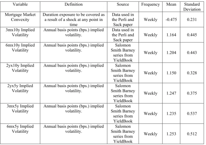
We use time series on the implied volatility for five swaptions: 3month x 5 year, 3 month x 10 year, 6 month x 5 year and 6 month x 10 year. The implied volatilities are measured in basis

points (bps.), i.e. 100th of one percent. The sources for the option volatilities were the Salomon

Smith Barney’s Yield Book online service or Perli and Sack. The time series for each of these volatilities was constructed as the product of daily rate volatility and the appropriate forward

rate.3 _{The descriptive statistics for the variables used and their definitions are described below in}

Table 1.

2 _{Swaptions are options contracts on a swap. These contracts provide the holder with an option to enter into a swap} at some point in the future. The quoted prices of these contracts are in volatility units, the market determined value of ex-ante volatility.

3 _{Basis point volatility for the 3 month x 10 year swaption equals the product of the rate volatility for the 3 month x} 10 year and the 3 month forward ten year rates.

8

Table 1: Definitions and Descriptive Statistics for Variables used in the Analysis: 1997:01 – 2003:054

The first two variables described in Table 1, mortgage market convexity and the convexity of the fixed income universe, measure the convexity exposure in terms of the magnitude of swaps that would have to be traded to remain duration neutral in the presence of a rate shock that is

typically 50 bps. We use the weekly observations on the mortgage market convexity measure, obtained from Perli and Sack to replicate their results. The remaining six weekly series measure implied volatility of both short and long-term swaptions.

Figure 1 displays both short and long volatility series. In examining the data we noticed that the Perli and Sack long implied volatility (2yx10y) series deviated from our series starting in 2001. While the Perli and Sack series differed in these later months they generally agreed with our pre-2001 data. To check the reliability of these series we obtained additional independent volatility data from JP Morgan and LehmanLive.com and found that their data more closely corresponded

4 _{The Annual basis points (bps.) implied volatility is divided by 100. In doing so we are staying consistent with} Perli and Sack (2003). Market convention, however, would express the implied volatility of a 3mx10y swaption as 116.4 basis points. This convention has no implications for the foregoing econometric exercise.

Variable Definition Source Frequency Mean Standard

Deviation Mortgage Market

Convexity Duration exposure to be covered as a result of a shock at any point in time

Data used in the Perli and

Sack paper Weekly -0.475 0.231 3mx10y Implied

Volatility

Annual basis points (bps.) implied volatility.

Data used in the Perli and Sack paper

Weekly 1.164 0.445 6mx10y Implied

Volatility Annual basis points (bps.) implied volatility. Smith Barney Salomon series from YieldBook

Weekly 1.204 0.443 2yx10y Implied

Volatility Annual basis points (bps.) implied volatility. Smith Barney Salomon series from YieldBook

Weekly 1.150 0.328 2yx5y Implied

Volatility

Annual basis points (bps.) implied volatility. Salomon Smith Barney series from YieldBook Weekly 1.247 0.375 3mx5y Implied

Volatility Annual basis points (bps.) implied volatility. Smith Barney Salomon series from YieldBook

Weekly 1.235 0.537 6mx5y Implied

Volatility Annual basis points (bps.) implied volatility. Smith Barney Salomon series from YieldBook

9

to our series than the Perli and Sack series over the 2001 to 2003 period.5 As a result of this

divergence we will consider model estimates using both the Perli and Sack series and the series using data from Salomon Smith Barney.

Figure 1: Time Series of the Perli and Sack and Our Values (Salomon Smith Barney) of Implied Volatility

First we replicate the first-stage results of Perli and Sack using their series and these findings are given in the first row of Table 2. Perli and Sack use the residuals from this first stage regression (after adding the average squared volatility) as the dependent variable in their second stage regression. Note that we numerically replicate their coefficient estimates.

The first set of results highlighted in first row of Table 2 below are obtained using Perli and Sack data, whereas, all the other results are obtained using our implied volatility series. It is

noticeable that using our series the value of the coefficients and the R2 are all significantly lower

than those obtained by Perli and Sack.6 We then re-estimate this first stage using the alternative

data series for both short and long volatility. These results are given in the second row of Table

5 _{The specification suggested in Perli and Sack requires that the volatility series be squared prior to the regression.} The post 2001 Perli and Sack volatility series more closely matched the square of our volatility series. This is suggestive of the possibility that the Perli and Sack data was updated with squared volatilities rather than volatilities. 6 _{We also note that after replicating the Perli and Sack first-stage results, the R}2 _{of 0.60 differed from the 0.95 value} reported in the Perli and Sack paper. It is important to note that this residual volatility is small both in relative and absolute magnitude. The average squared volatility is 1.07, of which the unexplained component is 0.21, with the coefficient of variation taking a value of 0.19, a small magnitude. In fact, it might be argued that this effect (of residual volatility) is so small that it not of any great consequence to any policy issues that relate to stability in financial markets. 0 1 2 3 4 5 6 1997 1998 1998 1999 2000 2001 2002 -1.6 -1.2 -0.8 -0.4 0 0.4 0.8 1.2 1.6 2 2.4

Perli & Sack 3month x 10year Salomon Smith Barney 3month x10year

Perli & Sack 2year x 10year Salmon Smith Barney 2year x10year

Left Hand Scale: 3month x 10yea

r

Right Hand Scale: 2year x 10year sqr

2year x 10year

3month x 10year

Perli & Sack

Salomon Smith Barney

Salomon Smith Barney

10

2 and qualitatively replicate the signs of the Perli and Sack coefficient estimates, but differs materially in their magnitude.

In order to evaluate the sensitivity of the Perli and Sack findings, we perform alternative first stage regressions using different swaption structures. The third row varies the Perli and Sack experiment by changing the short volatility series to one based on 6m x 10y swaptions. The fourth row varies the Perli and Sack experiment by shortening the long volatility series to the 2y x 5y swaption. The fifth and final row alters both series, taking the 6m x 5y swaption volatility as the short series and the 2y x 5y series as the long series. In these three cases the sign and the magnitude of the coefficients are similar to what was obtained in the replication of the Perli and Sack model using our short and long series. While there may be a difference between the results based on the data sources, we find that the first stage regressions produce similar results across the range of swaption volatilities that we explore. This suggests that these Perli and Sack findings are not specific to the particular swaption contracts they chose to explore.

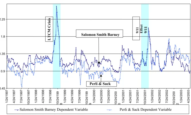
It is informative to examine the graph of the dependent variable created out of the first stage regression. Figure 2 plots the volatility series created by adding the residual from the first stage regression to the average squared volatility for the short-term swaption. Two features are striking in this graph. They are the spikes that occur the latter half of 1998 and near the end of 2001, associated with the LTCM and the 9/11 events. The LTCM extrema is approximately 6.54 standard deviation event and the 9/11 instance is a 3.77 standard deviation event. Since both least squares and Maximum Likelihood methodologies can be highly sensitive to outlier

observations, this graph motivates the exploration of the sensitivity of the Perli and Sack findings to these stressful episodes.

With the possibility of model error and parameter instability, the issues remains as to whether

any variability remains to be explained. However, most of our results do indicate that (with R2

ranging from .78 to .91) there may well be up to 22% of the variability that remains to be

explained. However, this is an issue that we will pursue in the next section.

Table 2: Regression Results for Short-Term on Long-Term Implied Variance

Estimated Parameters (p-values in Parenthesis) Dependent Variable Independent Variable Time Period Evaluated R-Square

0 ϕ ϕ₁ 3mx10yr 2yrx10yr 1997:01 – 2003:05 0.60 -0.631 1.827 -0.2811 1.2876 3mx10yr 2yrx10yr 1997:01 – 2003:05 0.7795 -0.2633 1.2765 6mx10yr 2yrx10yr 1997:01 – 2003:05 0.8892 -0.3891 1.3022 3mx5yr 2yrx5yr 1997:01 – 2003:05 0.8295 -0.3743 1.3051 6mx5yr 2yrx5yr 1997:01 – 2003:05 0.9143

11

Figure 2: Time Series Comparison of Perli and Our Dependent Variable

The exogenous variable used in this analysis is a proxy for hedging activity.7 The interest rate

risk in the universe of mortgage debt is measured by the total mortgage market duration and convexity. Starting from a duration neutral position for a given portfolio, the measure of hedging intensity will depend on the changes in the level of duration of mortgage debt. This change in duration will depend, in turn on the degree of convexity, as convexity is a measure of the rate of change of duration. As such, convexity serves as a reasonable proxy for changes in duration for investors who choose to dynamically hedge changes in duration.

It is worth noting that dynamic hedging is a reactive hedging protocol. However, most firms use a mixture of static and dynamic hedging. When rate changes alter the duration of assets, the portfolio can be rebalanced to a duration neutral position by changing the duration of liabilities, for example, by the use of swaps. To the extent that firms anticipate hedging needs and

eliminate some or all of the convexity exposure through the use of swaptions to offset the negative convexity inherent in the mortgage universe, the residual negative convexity would be the appropriate measure of hedging intensity. However, residual post-hedging convexity is unobservable and so the analysis uses mortgage market convexity. If firms change their mix of dynamic and static hedging during the sample period, this could diminish the predictiveness of this regressor.

7 _{Perli and Sack consider three proxies for hedging. Since they indicate that convexity is the most robust and} indicative measure of hedging intensity, we restrict our attention to this proxy.

0.45 0.9 1.35 1.8 2.25 1/24 /1997 4/24 /1997 7/24 /1997 10/24 /1997 1/24 /1998 4/24 /1998 7/24 /1998 10/24 /199 8 1/24 /1999 4/24 /1999 7/24 /1999 10/24 /199 9 1/24 /2000 4/24 /2000 7/24 /2000 10/24 /200 0 1/24 /2001 4/24 /2001 7/24 /2001 10/24 /2001 1/24 /2002 4/24 /2002 7/24 /2002 10/24 /200 2 1/24 /2003 4/24 /2003

Salomon Smith Barney Dependent Variable Perli & Sack Dependent Variable Salomon Smith Barney

Perli & Sack

LTCM Crisis

12

The series for convexity used in this paper is the same as that used by Perli and Sack. It provides a weekly measure of ten-year swap equivalents needed to swap out the changes in duration

resulting from changes in rates during the same period.8 We also use a broader measure of

convexity for the fixed income universe later in the estimation exercise, to provide a measure of the impact of the hedging needs of the fixed income universe.

An additional variable describing the magnitude of the convexity of the entire fixed income universe is used, and it measures the convexity of the all of the outstanding fixed income securities in the Broad Investment Grade (BIG) index. While the measure of convexity is of monthly frequency it does provide measure against which one can contrast the convexity of the mortgage universe and provide insight into the extent to which hedging in the fixed income universe might be contributing to volatility. When using this series to examine specific contribution of mortgages relative to the entire market, we will convert the mortgage market

convexity and implied volatilities to monthly observations.9

4. Impact of Mortgage Hedging on Volatility

Perli and Sack measure the impact of mortgage hedging on volatility by regressing the

constructed residual short-term volatility variable on a proxy for mortgage market hedging, the total mortgage market convexity. First, we replicate the Perli and Sack second-stage analysis and obtain coefficients that are identical and are presented in the first shaded row of Table 3. We then extend the second-stage analysis to different swaption structures. Using three other

swaption volatilities for the same sample period ( 6mx10yr, 3mx5yr, and 6mx5yr) we find that

we are able to obtain the estimates of the coefficients α₀ and α₁ that are nearly identical and

significant. For the parameter of interest, α₀β , the sign is in agreement with the results of Perli

and Sack for all of the swaption structures, but the magnitude is substantially reduced. We find that the estimates do not appear significant, but because the standard errors are not adjusted for heteroscedasticity, the reliability of inferences drawn is questionable.

Table 3: Regression Results for Orthogonalized Implied Variance Mortgage Market Convexity

As Independent Variable Estimated Parameters (p-values in Parenthesis) Dependent Variable Time Period Evaluated

0 α α₁ α₀β 0.1000 0.8856 -0.0846 3mx10yr 1997:01 – 2003:05 (0.00) (0.00) (0.00) 0.1511 0.8684 -0.0146 6mx10yr 1997:01 – 2003:05 (0.00) (0.00) (0.41) 0.1395 0.8746 -0.0314 3mx5yr 1997:01 – 2003:05 (0.00) (0.00) (0.22)

8_{Ten-year swap equivalents are a standard measure of the number of dollars of this contract that must be used to} eliminate a duration exposure.

13

0.1646 0.8597 -0.0228 6mx5yr 1997:01 – 2003:05

(0.00) (0.00) (0.22)

We move next to the estimation of the parameters using MLE with the specification described in (8). The MLE will be both efficient and provide a basis for asymptotically valid inference. The results for this exercise are described in Table 4 below. With the MLE estimation exercise we

are estimating four parameters: α₀, α₁, β and

υ

, and the parameter of interest is β , the

amplification parameter. For all of the swaption structures for this sample period, we find that

the coefficients are all highly significant and closely approximate the results of Perli and Sack.10

Table 4: MLE Results for Orthogonalized Implied Variance Mortgage Market Convexity

As Independent Variable Estimated Parameters (p-values in Parenthesis) Dependent

Variable Time Period Evaluated

0 α α₁

β

υ

0.0792 0.908 -0.834 0.0058 3mx10yr 1997:01 – 2003:05 (0.00) (0.00) (0.00) (0.00) 0.1093 0.892 -0.393 0.0037 6mx10yr 1997:01 – 2003:05 (0.00) (0.00) (0.01) (0.00) 0.0816 0.906 -0.917 0.0053 3mx5yr 1997:01 – 2003:05 (0.00) (0.00) (0.00) (0.00) 0.1273 0.879 -0.399 0.0039 6mx5yr 1997:01 – 2003:05 (0.00) (0.00) (0.00) (0.00)

One important test of a models’ validity is parameter stability. Intuitively, there maybe structural differences between periods with low levels of hedging activity as compared with periods of high levels of hedging activity. For example, in periods where the demand for hedging is low, risk managers may increase the proportion of hedging accomplished through static hedges. We proceed to examine this issue by segmenting the sample period into a period when the MBA Refi-index was low and with expected low levels of hedging activity and, a period when the MBA Refi-index was high and volatile, implying greater hedging pressures. For this purpose we split the sample period into two sub-samples, 1997:01 – 2000:12 and 2001:01 – 2003:05, and estimate the model for these two sub-periods.

It is here that we find a result that is counter-intuitive. During a period when the refi-incentives

were low and when we might have expected to find that the amplification parameter

β

to be low

in magnitude, yet we find it be to high not only for the 3mx10yr swaption structure, but for all of the others as well. Furthermore the estimates all have high p-values and t-statistics. Equally

10 _{We identified a problem with the specification of the Likelihood in the original Perli and Sack analysis, and} corrected it for the estimates provided in Table 4. The corrected Likelihood estimates did not materially differ. A derivation of the corrected Likelihood can be found in Appendix A.

14

counter-intuitive, for the period 2001:01 – 2003:05, when the MBA refi-index was high and

hedging pressures were great, we find that the values of the amplification parameter

β

implied

that higher levels of hedging actually lowered volatility. Furthermore these results are highly statistically significant. Were the original Perli and Sack specification correct, we would be unlikely to observe this magnitude of parameter instability.

Table 5: MLE Results for Orthogonalized Implied Variance Mortgage Market Convexity

As Independent Variable Estimated Parameters (p-values in Parenthesis) Dependent

Variable Time Period Evaluated

0 α α₁

β

υ

0.0529 0.930 -1.794 0.0038 1997:01 – 2000:12 (0.05) (0.00) (0.00) (0.00) 0.2958 0.838 0.476 0.0294 3mx10yr 2001:01 – 2003:05 (0.05) (0.00) (0.00) (0.00) 0.0671 0.928 -0.878 0.0025 1997:01 – 2000:12 (0.01) (0.00) (0.01) (0.00) 0.3319 0.784 0.292 0.0107 6mx10yr. 2001:01 – 2003:05 (0.01) (0.00) (0.02) (0.00) 0.0707 0.917 -1.334 0.0039 1997:01 – 2000:12 (0.01) (0.00) (0.00) (0.00) 0.2966 0.870 0.620 0.0467 3mx5yr 2001:01 – 2003:05 (0.04) (0.00) (0.00) (0.00) 0.0926 0.907 -0.714 0.0027 1997:01 – 2000:12 (0.00) (0.00) (0.00) (0.00) 0.3574 0.793 0.364 0.0135 6mx5yr 2001:01 – 2003:05 (0.00) (0.00) (0.01) (0.00)

To further refine our understanding of the parameter instability in the Perli and Sack model, we examine the parameter estimates of a rolling window. Specifically we take 123 week intervals starting with the first date 1997:01 and estimate the model parameters for each of data window. If the model were correctly specified, these estimates would be constant, except for sampling error. Alternatively, if the stability were caused by an outlier in the data, we would see

substantial movement in the parameter estimates as the outlier data points move into or out of the sample window.

Figure 3 below plots the amplification parameter estimate

β

as a function of the start date of the

123 week window. This graph exhibits two strong discontinuity points, one at about 3/31/1997

and the other at about 9/30/1998. These two points correspond to instances in which market disruptions brought about by LTCM enter and exit, respectively, from the sample window. Further, removing the few data observations associated with LTCM market disruption and re-estimating, results in coefficient estimates that shift from being variable and negative to positive, constant and frequently statistically significant.

15

Figure 3: Changing MLE Estimates of Sensitivity Parameter -6 -5 -4 -3 -2 -1 0 1 2 1/31/1997 4/30/1997 7/31/1997 _10/31/1997 1/31/1998 4/30/1998 7/31/1998 _10/31/1998 1/31/1999 4/30/1999 7/31/1999 _10/31/1999 1/31/2000 4/30/2000 7/31/2000 _10/31/2000

With spikes Without two spikes

6. Conclusion

Understanding volatility and its determinants is an important open issue. The possibility that risk mitigation strategies could have the unintended consequence of increasing the amplification of exogenous shocks to financial markets raises important policy questions. Perli and Sack ask an important question relating to mortgage risk management implications for interest rate volatility. Their analysis focused on explaining the component of short-term volatility unrelated to

movements in long-term volatility. While their empirical findings that linked mortgage hedging to increased volatility were an artifact of several outlier observations in the data, correcting their analysis by dropping periods associated with the LTCM crisis and 9/11, generate estimates that suggest there is little impact to the volatility from mortgage hedging. Indeed, over some periods the hedging activity appears to mitigate some of the market volatility.

While this analysis represents a step towards better understanding the linkage between hedging activities and financial stability, we believe that a more structural approach to this problem is needed. The term structure of volatility, for example, would suggest an alternative empirical approach to obtaining information about short-term volatility unrelated to long-term volatility movements than was taken in the Perli and Sack first stage regression. Further, the component of short-term volatility not explained by movement in long-term volatility is small in both

LTCM Effect

16

absolute and relative magnitude. Any theory that has policy relevance needs to explain material movements in market volatility.

17

Appendix 1

For a variable x that follows normal distribution ( , 2)

x x

N µ σ , with mean µ_x and variance σ_x2,

the likelihood function, or the density function, is as follows: ) 2 ) ( exp( ) 2 ( 1 ) ( ₂ 2 2 1 x x x x x f L σ µ σ π − − = = .

The log-likelihood function is the result of taking natural log on both sides of the above equation:

2 2 2 ) ( 2 1 ln 2 1 2 ln 2 1 log _x x x x L µ σ σ π − − − − = .

To maximize log is to maximize L 2

2 2 ) ( 2 1 ln 2 1 x x x x µ σ σ − − − .

From equation (7) we have: _{r t} X _t 2_{r t} (1 X_{t 1})u_t

1 , 1 1 0 0 2 , − ∆ − − ∆ =α +α β +α σ + + β σ .

We can use ε_t to denote the amplified error term, withε_t =(1+βX_t−1)u_t. ε_t follows normal

distribution (0, (1 )2) 1 − + X_t V N β .

Our x variable here is 2

,t r ∆ σ , with 2 1 2 ) 1 ( + ₋ = _t x V βX σ and

(

)

2 1 , 1 1 0 1+ − + ∆ − = _{t rt} x α βX ασ µ .

Substitute these terms into the log-likelihood function, we have:

(

)

(

(

)

)

(

)

(

(

)

₂

)

2 1 , 1 1 0 2 , 2 1 2 1 1 0 1 1 2 1 1 ln 2 1 , , , _{∆ − ∆ −} − − − + − + − + − = _{rt t rt} t t X X X L σ α β ασ β υ β υ υ β α α , instead of

(

)

(

(

)

)

(

(

)

₂

)

2 1 , 1 1 0 2 , 2 1 1 0 1 2 1 1 ln 2 1 , , , =− + X_t− − _∆rt − + X_t− − _∆rt− L σ α β α σ υ β υ υ β α α as in equation (8).

18

References

De Long, Bradford, Andrei Schleifer, Lawrence H. Summers and Robert J. Waldmann, “Positive Investment Feedback Strategies and Destabilizing Rational Speculation,” Journal of Finance, v. xlv, no. 2, June 1990.

Dunbar, Nicholas, “Inventing Money: The Story of Long-Term Capital Management and the the Legends Behind It,” John Wiley & Sons; New Edition 2001.

Friedman, Milton, Essays in Positive Economics. Chicago: Univ. of Chicago Press, 1953. Hart, Oliver D., David M. Kreps, “Price Destabilizing Speculation,” Journal of Political

Economy, pp. 927-952, v. 94, no. 5, 1986.

Jorion, Phillipe, “Fallacies in the Effects of Market Risk Management Systems,” Working Paper, July 2002.

Naranjo, Andy and Alden Toevs, “The Effects of Purchases of Mortgages and Securitization by Government Sponsored Enterprises on Mortgage Yield Spreads and Volatility,” pp. 173-195, Journal of Real Estate Finance and Economics, Sept.-Dec. 2002, v. 25, iss. 2-3. Perli, Roberto and Brian Sack, “Does Mortgage Hedging Amplify Movements in Long-Term

Interest Rates?” pp. 7-17, Journal of Fixed Income, Dec. 2003.

Persaud, Avinash, “Sending the Herd Off the Cliff Edge: The Disturbing Interaction Between Herding and Market Sensitive Risk Management Practices,” Journal of Risk Management Practices,” Journal of Risk Finance 2, 59-65, 2000.