Why do stock prices drop by less than the value of the dividend? Evidence from a country with a flat tax rate on capital gains and dividends.

Full text

(1)Master’s Thesis in Finance. Why do stock prices drop by less than the value of the dividend? Evidence from a country with a flat tax rate on capital gains and dividends. Jonathan Israelsson and Max Wann-Hansson. Graduate School Supervisor: Taylan Mavruk Spring 2017.

(2) Abstract We examine the effect of taxes, trading activity and different market microstructures on the exdividend day stock price behaviour. Based on previous literature, we build our hypotheses and test them on 1380 ex-dividend day observations in order to pinpoint the explanations behind the empirical findings on the Stockholm Stock Exchange over the period 2007 to 2016. We find price-drop ratios of 72% and 56% in the close-to-close sample and close-to-open sample, respectively. This finding opposes the theoretically implied price-drop ratio of one given the prevailing tax regime in Sweden. The trading activity increases around the ex-dividend day and is the greatest in high-yield stocks. We also find that the price-drop ratio is positively related to dividend yield, indicating that stock prices are set more efficiently in high-yield stocks on the ex-dividend day. Our findings are generally consistent with the short-term trading explanations from previous literature. Transactions costs seem to be the factor limiting the stock prices to drop by the value of the dividend. It is also possible that ex-dividend day stock prices are affected by factors that has not been discovered by financial literature.. We would like to thank our supervisor Taylan Mavruk for his kind help, patience and guidance throughout this process. The input he has provided has been an important support during this period.. 1.

(3) Table of Contents 1. Introduction ................................................................................................................. 3 2. Previous research and hypotheses development .......................................................... 5 2.1 Tax .................................................................................................................................... 5 2.2 Market microstructures ..................................................................................................... 7 2.2.1 Tick size ................................................................................................................................. 7 2.2.2 Limit-order adjustments......................................................................................................... 8 2.2.3 Transaction costs ................................................................................................................... 9 2.3 Short-term trading ............................................................................................................ 9 2.4 Summary of previous findings ......................................................................................... 11. 3. The Swedish taxation system ..................................................................................... 12 4. Data and variables ..................................................................................................... 12 4.1 Data ................................................................................................................................. 12 4.2 Summary of variables ...................................................................................................... 14. 5. Methods ..................................................................................................................... 15 5.1 Testing the tax hypothesis ................................................................................................ 15 5.2 Testing market microstructure hypotheses ...................................................................... 16 5.2.1 Testing the tick-size hypothesis ........................................................................................... 16 5.2.2 Testing the limit-order adjustments hypothesis ................................................................... 17 5.2.3 Testing the transaction costs hypothesis .............................................................................. 17 5.3 Testing the short-term trading hypothesis ....................................................................... 18 5.4 Regression model ............................................................................................................. 18. 6. Results and analysis ................................................................................................... 20 6.1 Descriptive statistics and univariate results ..................................................................... 20 6.1.1 Descriptive statistics and analysis of tax ............................................................................. 20 6.1.2 Descriptive statistics and univariate results of market microstructures ............................... 22 6.1.3 Descriptive statistics and univariate results of short-term trading ....................................... 23 6.2 Regression analysis .......................................................................................................... 26 6.3 Summary of results .......................................................................................................... 30. 7. Robustness ................................................................................................................. 31 8. Conclusion ................................................................................................................. 32 9. References .................................................................................................................. 34 10. Appendix .................................................................................................................. 36. 2.

(4) 1. Introduction In a perfect and frictionless capital market, where there is no uncertainty, the stock price should fall by an amount equal to the value of the dividend on the first day the stock is traded without the right to receive the next dividend (Akhmedov and Jakob, 2010). There is a large number of studies on the stock price behaviour around the ex-dividend day, where most studies find that the stock price on average drop by an amount less than the value of the dividend (Akhmedov & Jakob, 2010; Bali & Hite, 1998; Elton et al, 2005; Frank & Jagannathan, 1998). For example, on May 13, 2014, Kinnevik B shares had their first trading day without the right to receive the most recently announced dividend of 7 SEK. That day, the stock price only decreased by 2.1 SEK. In an efficient market, there should be no possibility of arbitrage. This thesis aims to address the following question: Why do stock prices drop by less than the value of the dividend?. In this thesis, we test various factors impacting the stock price behaviour around the ex-dividend day on the Stockholm Stock Exchange (SSE). Understanding the behaviour of the stock price around the ex-dividend day has important implications for market efficiency and theoretical frameworks in financial economics (Akhmedov & Jakob, 2010). The most commonly used metrics to measure stock price behaviour on the ex-dividend day are abnormal returns and the price-drop ratio, defined as the ratio of the drop in stock price divided by the dividend amount. A price-drop ratio less than one on the ex-dividend day has generally been explained as an effect of taxes. In the U.S., where most studies are conducted, investors face more favourable tax treatment of capital gains than on dividends (Elton et al, 2005). According to the tax explanation, this affect the investors’ preferences for dividends and ultimately result in a pricedrop ratio of less than one.. Daunfeldt, Selander and Wikström (2009) and Palm and Selinus (2007) examine the tax effect on the SSE during the 1990’s, when capital gains and dividends were taxed differently. Both find a price-drop ratio less than one but that tax has little or no effect on the price changes. The tax explanation remains contested and provided with a range of alternative explanations. The Swedish tax regime has remained unchanged since the year of 1995, with flat and equal tax rate on capital gains and dividends (30%). This provides a good setting to examine factors impacting price behaviour around the ex-dividend day. Hedman and Moll (2006) examine factors that affect the ex-dividend day price behaviour on the SSE during 2001 to 2005. Their result show. 3.

(5) that a market microstructure, in form of tick size, seem to affect the stock price behaviour on ex-dividend day. There are several lines of reasoning based on market microstructures to explain the ex-dividend day anomaly (Akhmedov and Jakob, 2010). These explanations show that, even in the absence of differential taxes, stock prices drop by less than the value of the dividend. We therefore investigate whether a group of market microstructures affect the stock price behaviour around the ex-dividend day: (1) tick size, (2) the lack of limit order adjustment, (3) transaction costs.. According to Elton et al (2005), a price-drop ratio less than one should generally result in abnormal returns. This attracts short-term traders who trade until the remaining abnormal return represent the marginal transaction costs associated with arbitrage trading (Kalay, 1982). Therefore, we also investigate the presence of short-term traders around the ex-dividend day and whether they affect the price-drop ratios.. None of the previous studies on the SSE are able to fully explain the price-drop anomaly. The purpose of this thesis is to find the factors impacting the stock price behaviour on the exdividend day in hope of giving a better explanation to why stock prices drop by less than the value of the dividend. The analysis is delimited to the Stockholm Stock Exchange during the period 2007 to 2016 and stocks listed on the main market. In contribution to previous studies on the Swedish market, we first analyse the previously unexamined effect of the lack of an automated limit order adjustment on the SSE. Akhmedov and Jakob (2010) hold low liquidity levels in combination with the lack of an automated limit order adjustment as their main explanation for the price-drop anomaly on the CSE. We believe the CSE and SSE are very similar in their characteristics, making this mechanism interesting to examine. Second, we analyse data in the period during and post the financial crisis, which has not been done previously on the SSE. The trading volume has increased dramatically in the last decade, making new data interesting to examine. Third, data on opening prices enable us to examine the overnight price-drops and intraday changes in the price-drop ratio. Fourth, we also explicitly look at transaction costs impact on the ex-dividend day price behaviour through a proxy never used on the SSE before. Finally, our dataset is also, to the best of our knowledge, the most extensive one ever to be examined on the SSE. Internationally there have been few studies simultaneously examining the impact from tax, a group of market microstructures and short-term traders, with Akhmedov and Jakob (2010) as. 4.

(6) an exception. We use their paper as a reference point throughout this thesis and compare our results with their findings from the Danish market. Our result shows a price-drop ratio of 72%. Our findings indicate that short-term traders seem to be present around ex-dividend day and that the price-drop anomaly is explained by transaction costs. We begin this thesis with a review of previous literature. Based on the literature review, we state our hypotheses and build our data section. The subsequent sections present the methodology and the results from both descriptive data and regression analysis. We then discuss the robustness of our results and end this thesis with a summary and conclusion of our findings.. 2. Previous research and hypotheses development We divide the literature review into three different subsections, where each group of empirical explanations for the price-drop anomaly will be discussed in turn. We build our hypotheses based on the theoretical predictions in the literature review.. 2.1 Tax In 1961, Modigliani and Miller introduced the clientele effect, stating that investors make their investment decisions based on the dividend policy. Under many tax regimes, investors have different rates of taxation on capital gains and dividends. The implication is that investors prefer different optimal dividend policies. In those tax regimes where dividends are taxed heavier than capital gains, a dollar of capital gains must be worth more than a dollar of dividend (Daunfeldt et al, 2009). This effect was studied by Elton and Gruber in 1970. They show how the marginal investor’s tax bracket can be derived by studying the ex-dividend day stock price behaviour. In an equilibrium market, the ex-dividend stock price behaviour must be such that it leaves the potential buyers indifferent as to whether they should buy the stock before or after its exdividend day. This relationship is expressed in equation 1: 𝑃𝑡−1 − 𝑡𝑐 (𝑃𝑡−1 − 𝑃𝑝 ) = 𝑃𝑡 − 𝑡𝑐 (𝑃𝑡 − 𝑃𝑝 ) + 𝐷(1 − 𝑡𝑑 ). (1). Where: Pt-1 = Stock price on the day before the ex-dividend day Pt = Stock price on the ex-dividend day PP = Purchase price of the stock td = Tax rate on dividend income tc = Tax rate on capital gains D = Dividend amount. 5.

(7) The left-hand side in equation 1 represents the per share wealth gain from selling the day before the ex-dividend day (i.e. cum-dividend day). Since the investor cares about after-tax return, this must equal the right-hand side in an equilibrium market, which represents the wealth gain from selling on the ex-dividend day. That is, if the investor sells the shares on the day before the exdividend day, he must receive the price of the stock minus the tax on the capital gains. If he, on the other hand, sells the stock on the ex-dividend day, he receives the dividend minus the tax on dividend, plus the capital gains minus the capital gains tax. A higher tax rate on dividends than on capital gains will thus lead to a price drop smaller than the dividend. Given this relationship, ex-dividend day stock price behaviour can give information about the tax brackets of the investors in the firm (Elton and Gruber, 1970). Equation 1 can be rearranged:. 𝑃𝑡−1 − 𝑃𝑡 1 − 𝑡𝑑 = 𝐷 1 − 𝑡𝑐. (2). The left-hand side of equation 2, the price-drop ratio, represent an expression for the theoretically implied drop in stock price on the ex-dividend day. Given different tax rates as inputs in the right-hand side of the equation, the left-hand side will give different implied pricedrops. Whenever the tax rate for capital gains is higher than the tax rate on dividends (i.e. tc>td), the price-drop ratio will be above one. If the tax rate on capital gains is less than the tax rate on dividends (i.e. tc<td), the numerator of the right-hand side of the equation will be smaller than the denominator, resulting in a price-drop ratio less than one.. Different tax preferences might form tax clienteles. If such tax-clienteles form, the price-drop ratio will have a positive relationship with dividend yield. Elton and Gruber (1970) find that the average price drop ratio on the New York Stock Exchange (NYSE), between April 1966 and March 1967, is approximately 78% and that the probability of a value of one or more was less than 1.5%. They also find a relationship between high dividend yields and high price drop ratios. Elton and Gruber (1970) believe these results give support to tax-clientele effect, such that the price drop ratio is less than one if the marginal investor’s tax rate is higher on dividend income than on capital gains. Several studies provide support for the tax explanation (Elton & Gruber, 1970; Elton et al, 2005; Graham, Michaely & Roberts, 2003; Haesner & Schanz, 2013).. 6.

(8) Daunfeldt et al (2009) and Selinius and Palm (2007) study the effect of differential taxes on the SSE in 1991 to 1995 and 1991 to 2000, respectively. During these periods, Sweden subsequently changes the tax regime three times. Their results show no indication of tax effects on the ex-dividend day stock price behaviour. The Swedish taxation system has remained unchanged since 1995, with flat and equal tax rate on dividends and capital gains (i.e. td=tc in equation 2). If the tax explanation is valid, the price drop ratio should be equal to one in all years since 1995 (Daunfeldt et al, 2009). That is, if we insert the prevailing tax rate in Sweden into the right-hand side of equation 2, the price should fall by the exact amount of the dividend as if there were no taxes at all. Otherwise arbitrage opportunities might arise in the market. Based on the tax explanation, we arrive at our first hypothesis:. H1: According to the tax hypothesis, the price-drop ratio should equal one given the Swedish taxation system. 2.2 Market microstructures In addition to the tax hypothesis, another group of research articles rely on different market microstructure characteristics as explanations for an ex-dividend day price-drop ratio of less than one. This group argues that, even in the absence of progressive and differential taxes, they find that the stock prices drop by less than the dividend. This section gives a review of three of the most prominent market microstructure explanations used in previous research. Hypotheses are built on the theoretical predictions for each market microstructure.. 2.2.1 Tick size The first market microstructure alternative is the tick size hypothesis, proposed by Bali and Hite in 1998. They examine the fact that dividends on the NYSE is not always a multiple of the tick size, which cause the non-continuous pricing on ex-dividend day. A tick is the minimum amount a stock can change in price. At the time of Bali and Hite’s (1998) study, tick size was set to 1/8 on the NYSE. The result from their study show that the price drop is less than the dividend but at the same time equal to or greater than the dividend minus the tick size. Bali and Hite argue that the tick causes a stock price change that is rounded to nearest tick below the dividend. This explanation is supported by Frank and Jagannathan (1998), who find that the tick-size causes the price-drop anomaly. In Sweden, Hedman and Moll (2006) find further support for the tick size explanation on the SSE.. 7.

(9) Graham et al (2003) analyse the tick size model’s liability as the pricing grid dramatically changed from 1/8 to 1/16 to decimals. They argue that, with the new decimal tick sizes, the tick-size model by Bali and Hite (1998) should suggest a price-drop ratio closer to one. However, their result show the opposite. This result is also in line with the findings of Akhmedov and Jakob (2010). They do not find any support for the tick size explanation when examining the Danish exchange market. An example of Bali and Hite’s (1998) tick size explanation is that if the dividend is 20 cents and the tick size is 12.5 cents, it would lead to a 12.5 cent drop in the stock price. The price falls to the nearest tick below the dividend, in this case 12.5 cents. Resulting in a price-drop ratio of 0.625. As the Danish exchange market, the tick sizes on the SSE decrease with increasing market value of the company (see appendix 4). Based on theoretical predictions of Bali and Hite (1998), that tick sizes have an impact on the stock price behaviour on the exdividend day, we arrive at the following hypothesis:. H2: Based on the tick-size hypothesis, the price drop ratio should be lower for observations where the tick size is not an exact multiple of the dividend. 2.2.2 Limit-order adjustments In addition to the tick size explanation, Dubofsky (1992) suggest that the automated limit order adjustment existing in the United States control the behaviour of ex-dividend day stock prices. The automated limit order adjustment adapts outstanding limit buy orders from cum-dividend day to ex-dividend day downward with the dividend amount to the nearest tick size. However, limit sell orders are not adjusted. Dubofsky (1992) argues that this mechanism’s impact on the limit order book, drive the price-drop ratios and has positive impact on them. An example of this mechanism is if the size of the tick is 0.0625 cents and the dividend is 0.10 cents. The automated mechanism will then adjust the limit buy orders down by 0.125 cents. Jakob and Ma (2004) studies the price-drop ratios on the Toronto Stock Exchange (TSX), which does not have this automated limit order adjustment mechanism. According to them, the two main reasons why there exist incomplete adjustments of the stock price on the TSX are the lack of an automated limit order adjustment and low trading volumes in comparison to those found in the U.S by Dubofsky (1992). Akhmedov and Jakob (2010) test this model on the Copenhagen Stock Exchange (CSE) and conclude that the main drivers for price-drop anomaly on ex-dividend day is the lack of an automated limit order adjustment mechanism and relatively low liquidity.. 8.

(10) The SSE also lacks this automated limit order adjustment mechanism, which should drive the price-drop ratio towards one. Higher normal liquidity in a stock should, according to Akhmedov and Jakob (2010), compensate for this by lessening the influence of outstanding limit orders. Manual adjustments from investors and new orders over night are, according to Dubofsky (1992) and Jakob & Ma (2004), more likely if there exist higher levels of market liquidity. From the theories and findings outlined above, we derive the following hypothesis for the lack of an automated limit order adjustment: H3: The absence of an automated limit order adjustment mechanism, predicts a pricedrop ratio of zero. As liquidity levels should compensate for the lack of an automated mechanism, normal trading volume should have a significant positive impact on the price-drop ratio. 2.2.3 Transaction costs A third group of microstructure explanations argues, that even in the absence of differential taxes, transaction costs limit the stock price to drop by the value of the dividend. Frank and Jagannathan (1998) examine this implication on the Hong Kong market, where there are no taxes on capital gains and dividends, and argues that a price-drop ratio less than one must stem from market microstructure effects and transaction costs. A price-drop ratio less than one implies that the excess return on the ex-dividend day is positive. According to Karpoff and Walkling (1988), the risk-adjusted returns on the ex-dividend day are positive and represent profit opportunities for arbitrage short-term traders. Therefore, short-term traders should engage in trading until the marginal transaction cost equals the abnormal returns. Based on this theory, transaction costs above zero implies a price-drop ratio of less than one and that the price-drop ratio should be negatively related to the transaction costs (Karpoff and Walkling, 1988): H4: There should be a negative relationship between transaction costs and price-drop ratio on the ex-dividend day.. 2.3 Short-term trading The tax explanation and market microstructures explanations suggest a price-drop ratio of less than one. The short-term trading hypothesis is based on the view that some investors are arbitrage traders and tax-neutral to capital gains and dividends. An expected price-drop ratio less than one represents an arbitrage opportunity to those investors (Kalay, 1982). If the arbitrage opportunity is exploited, it should limit the stock price change on the ex-dividend day. 9.

(11) (Elton et al, 2005). Therefore, the price-drop ratio reflects the transaction costs of those traders and cannot be used to infer marginal tax rates (Karpoff and Walkling 1988; Lakonishok and Vermaelen, 1986). In the tax-clientele model, institutional investors may face different dividend tax rates than individuals and prices are set by investors who trade with reasons unrelated to the dividend. Kalay (1982) state that these tax differences can be exploited by institutions to make a profit and that the size of the profit is positively related to the dividend yield. Therefore, a positive relationship between the price-drop ratio and the dividend yield can be a result of either tax-induced trading or arbitrage trading (Lakonishok & Vermaelen, 1986). With progressive taxes, it is not possible to distinguish between tax-induced trading and short-term arbitrage trading, since they are both likely to increase trading volumes around the ex-dividend day (Haesner and Schanz, 2013).. In Sweden, abnormal trading volume must be motivated by arbitrage trading (Daunfeldt et al, 2009). Akhmedov and Jakob (2010) argues that this abnormal trading activity will push the price ratio towards one. To determine the importance of short-term traders, we will test for abnormal trading volumes around the ex-dividend day. This leads to our next hypothesis: H5a: According to the short-term trading hypothesis, there should be abnormal trading around the ex-dividend day. In addition, the price-drop ratio should be equal to one. If differential taxes affect investors’ preferences for dividends, those investors with relatively low marginal tax rate on dividends would prefer stocks with high dividend yield. Tax-clienteles among investors would take form. In such instances, the price-drop ratio increases with dividend yield (Elton and Gruber, 1970). However, under the prevailing Swedish tax regime, a positive relationship between the price-drop ratio and dividend yield cannot be explained by tax-clienteles (Daunfeldt et al, 2009). A positive relationship between the price-drop ratio and dividend yields on the SSE must rather come from arbitrage trading driven by the relative importance and attention to larger dividends. Kalay (1982, 1984) show that the arbitrage profits are increasing with dividend yield and that high dividend yield stocks should attract more shortterm traders.. 10.

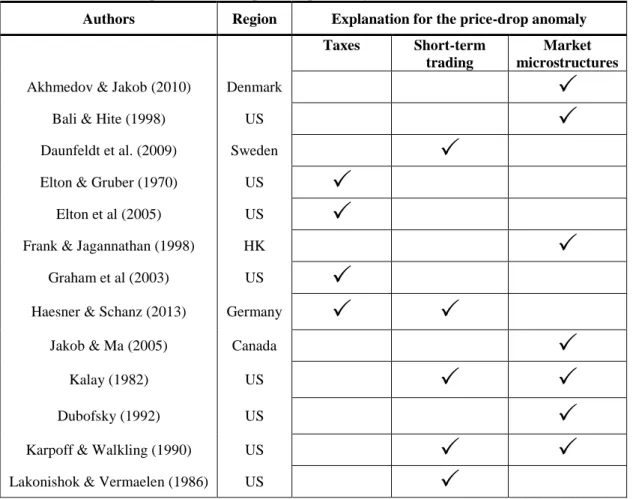
(12) At high dividend yields most investors pay attention, and the tick size and transaction costs have less impact on the price setting, which ultimately would lead to more efficient price setting on the ex-dividend day (Frank and Jagannathan, 1998). As a consequence of this discussion, our next hypothesis is the following:. H5b: The price-drop ratio for SSE-listed firms is increasing in dividend yield. 2.4 Summary of previous findings We summarize some of the most important previous research based on their different findings in table 1 below. The majority of studies use the price-drop ratio provided by Elton & Gruber (1970), when studying the price behaviour around the ex-dividend day. All listed studies find that the stock prices drop by less than the value of the dividend on the ex-dividend day. However, the explanation for this price-drop anomaly differs a lot between studies.. Table 1 Previous findings The table give an overview of the empirical findings of published papers. All listed studies find a price-drop ratio less than on. The explanations to the price-drop anomaly are market with check marks. Authors. Region. Explanation for the price-drop anomaly Taxes. Akhmedov & Jakob (2010). Denmark. Bali & Hite (1998). US. Daunfeldt et al. (2009). Sweden. Elton & Gruber (1970). US. Elton et al (2005). US. Frank & Jagannathan (1998). HK. Graham et al (2003). US. Haesner & Schanz (2013). Germany. Jakob & Ma (2005). Canada. Kalay (1982). US. Dubofsky (1992). US. Karpoff & Walkling (1990). US. Lakonishok & Vermaelen (1986). US. Short-term trading. Market microstructures.        .    .    . 11.

(13) 3. The Swedish taxation system Since the tax reform in 1991, individual tax rate on capital income is flat at 30% (The Swedish tax agency, 2017). This tax rate applies to both dividend income and capital gains. In the absence of a tax treaty, non-residents are subject to the same tax rate of 30% on dividend income. Legal entities in other EU member states owning more than 10% of the capital in a Swedish company are exempt from withholding tax. These tax rates imply that the marginal investor, under the Swedish tax regime, pay equal tax rates on dividends and capital gains. Therefore, the price-drop ratio should be equal to one.. Swedish companies generally pay dividends once a year. Given that the whole dividend is distributed only once a year, it should be good conditions to study the price behaviour around the ex-dividend day. In Sweden, public companies normally have their Annual General Meeting such that it coincides with the cum-day. This event involves certain elements that might affect the stock price. In some cases, new information or guidance is released. Although it is usually already established, the final decision regarding the dividend is also taken at the Annual General Meeting.. 4. Data and variables In this section, we first present our database and definitions used throughout this thesis. Second, all variables used in tests and analysis are described with a summary table.. 4.1 Data The main data source is the Compustat database. It provides global financial information on active and inactive companies. Our dataset consists of all stocks listed at the Stockholm Stock Exchange main market that distributed dividends at least two years between the years 2007 and 2016. In line with Akhmedov and Jakob (2010) we exclude stocks with only one year of dividends because they can generate noisy data. From Compustat we gather daily closing prices, dividend amounts and daily trading volumes for all stocks in the sample. To construct our variables, we need data from the cum-dividend day and the ex-dividend day. The cum-dividend day represents the last day the stock is traded with its dividend right. In Sweden, this day is three trading days before the actual record date, since there is a three-day settlement delay. The ex-dividend day is the first trading day the stock is traded without its dividend right, i.e. the day after the cum-dividend day. 12.

(14) We have collected information about the cum-dividend day and ex-dividend dates from either Compustat or, in those cases where data was missing, from the companies’ investor relations homepage. All dividends in the sample are annual dividends.. Since Compustat do not give information on daily opening stock prices, the sample is complemented with opening stock prices from NASDAQ OMX Nordic’s official database. Our dataset ranges from 2007 to 2016. However, NASDAQ’s database only contains data on daily opening stock prices from 2008, which limit our sample of close-to-open data to nine years (2008-2016). The raw dataset consisted of 1433 close-to-close observations and 1272 close-toopen observations1. After excluding those observations with missing values in other secondary variables, such as cum-dividend day volume and ex-dividend day volume, the final dataset consists of 1380 close-to-close observations and 1247 close-to-open observations.. The sample only contains observations with stocks distributing cash dividends (either regular or extra) paid in Swedish krona2. Other kinds of dividends that are not cash dividends are excluded3. When a regular and an extra cash dividend are distributed on the same date, these are aggregated to one observation.. To limit the effect of noisy outliers the final dataset is globally winsorized at 1% (0.5% of the lowest values and 0.5% of the highest values). In contradiction to trimming or excluding the most extreme outliers, winsorizing is transforming these outliers to a certain percentile. Thus, the extreme outliers are replaced by the maximum and minimum. In our case the 0.5th percentile and the 99.5th percentile.. 1. Close-to-close are price-drop ratios computed from cum-dividend day close price to ex-dividend day close price. Close-to-open are price drop-ratios computed from cum-dividend day close price to ex-dividend day open price. 2 Cash dividends paid out in a foreign currency are excluded because of exchange-rate effects. 3 Other kind of dividends are such as stock splits and stock dividends. These are excluded as one cannot measure the tax effect and will therefor give the price-drop ratio a skewness.. 13.

(15) 4.2 Summary of variables In table 3, all variables used to test our hypothesis are summarized. Most variables are in line with those of Akhmedov and Jakob (2010). However, as the transaction cost hypothesis is included in our analysis, market value and outstanding shares are also included. Table 3 Summary of variables Variables. Description. Price-drop ratio. Measures the ratio of change in price between the cum-dividend day and ex-dividend day to the dividend amount. AMR. The price-drop ratio adjusted for market movements. AR. Measures how much the return on an individual stock exceeds the market return between cum-dividend day and ex-dividend day. Dividend yield. Dividend amount as a percentage of the cum-dividend day stock price. Market return. The return of OMXSPI stock market index. A_REG. Total average trading volume around ex-dividend day divided by normal trading volume. E_REG. Total daily trading volume on ex-dividend day divided by normal trading volume. C_REG. Total daily trading volume on cum-dividend day divided by normal trading volume. Tick size dummy. Dummy variable with value of 1 if tick size is not a multiple of the dividend and 0 otherwise. Predicted ratio. Expected price-drop ratio based on the tick-size hypothesis by Bali & Hite (1988). Market value. Outstanding shares multiplied with stock price on cum-dividend day. Outstanding shares. Number of outstanding shares on cum-dividend day. 14.

(16) 5. Methods In this section, the methodologies for testing the hypotheses are explained.. 5.1 Testing the tax hypothesis The tax explanation by Elton and Gruber (1970) can be applied to and tested by the price-drop ratio. The price-drop ratio measures the change in stock price between the cum-dividend day and ex-dividend day as a fraction of the dividend. It gives an indication of how much the stock price drops in comparison to the dividend amount. The price-drop ratio will represent the main variable in our analysis.. Price − drop ratio =. 𝑃𝑡−1 − 𝑃𝑡 𝐷. (4). Where: Pt-1 = Stock price on the day before the ex-dividend day Pt = Stock price on the ex-dividend day D = Dividend amount. Given equation 2, the price-drop ratio should be one in our sample. To test the tax hypothesis, we conduct a z-test where the null hypothesis is a price-drop ratio with a mean of one, and the alternative hypothesis is a mean different from one. If the price-drop ratio is significantly different from one, we can reject the tax hypothesis. We gather data on both close-to-close and close-to-open price-drop ratios and test if there is a significant difference between them in order to determine potential discrepancies caused by the intra-day trading. To determine if the means are different in the two samples, a z-test is conducted.. The market-adjusted price-drop ratio (AMR), as outlined by Akhmedov and Jakob (2010), is important because market return can have an impact on the individual stock price on the exdividend day. The AMR controls for these market movements by adjusting the stock price on the cum-dividend day by the market return on the ex-dividend day. In line with Akhmedov and Jakob (2010), we use a market capitalization weighted price index, OMXSPI, as a proxy for market return. The ratio is calculated in the following way, where rm is the market return:. AMR =. 𝑃𝑡−1 × (1 + 𝑟𝑚 ) − 𝑃𝑡 𝐷. (5). 15.

(17) Several papers use abnormal returns as an alternative, or complement, to the price-drop ratio (Akhmedov and Jakob, 2010). If the individual stock price drops by less than the value of the dividend, the stock has to exhibit abnormal returns. Market wide returns can have great effects on the stock prices during the day. Therefore, the abnormal returns formula is calculated such that it is positive only if abnormal returns on the ex-dividend day exceeds the return of the market. With flat and equal tax rates, we expect abnormal returns equal to zero. This is tested by conducting a z-test. We calculate abnormal return for individual stocks at the ex-dividend day as the following:. 𝐴𝑅 =. 𝑃𝑡 − 𝑃𝑡−1 + 𝐷 − 𝑟𝑚 𝑃𝑡−1. (6). 5.2 Testing market microstructure hypotheses 5.2.1 Testing the tick-size hypothesis The model by Bali and Hite (1998) states that, if the tick-size constraints affects the price-drop ratio, the stock price should fall to the nearest tick amount below or equal to the amount of the dividend on the ex-dividend day. As tick sizes in both Denmark and Sweden change with the stock price, we use the formula calculated by Akhmedov and Jakob (2010) to determine the predicted price-drop ratio for each dividend according to the tick size model. The predicted price-drop ratio, based on the tick size explanation by Bali and Hite (1998), is the following:. 𝑃𝑟𝑒𝑑𝑖𝑐𝑡𝑒𝑑 𝑟𝑎𝑡𝑖𝑜𝑡 =. [𝐼𝑛𝑡(Dt ÷ Tick t )] × (𝑇𝑖𝑐𝑘𝑡 ) 𝐷𝑡. (3). Where: Dividend = Dividend amount Tick = Tick-size Int (X) = Integer, i.e. value in parenthesis rounded downward to nearest whole number. If the tick-size is an exact multiple of the dividend the predicted ratio in equation 3 will equal one, otherwise it will be less than one.. 16.

(18) We test the tick size hypothesis in two ways. First, we use equation 3 to calculate the predicted price-drop ratios for all dividends, conduct a z-test to determine if the predicted price-drop ratio is significantly less than one and then compare the predicted ratio with the observed price-drop ratios in the sample. If the tick size explanation is the only thing explaining the price-drop anomaly, we should observe price-drop ratios consistent with the predicted ratios. Second, in line with Jakob and Ma (2005), a regression analysis examines the impact of tick size on the price drop ratio. This is measured with a tick size dummy, which is given the value of 1 if the dividend is not an exact multiple of the tick size and 0 if it the dividend is an exact multiple of the tick size. For the tick size hypothesis to hold, the dummy coefficient must be negative and significant to indicate that stocks with a dividend that is not an exact multiple of the tick size should have lower price-drop ratios. 5.2.2 Testing the limit-order adjustments hypothesis The SSE lack an automated adjustment mechanism limit orders. According to Jakob and Ma (2005), this should limit the drop in stock price and thereby result in lower price-drop ratios. The normal trading volume, a measure of liquidity in an individual stock in its normal state, should have a significant positive impact on the price-drop ratio. Therefore, in line with Jakob and Ma (2005) and Akhmedov and Jakob (2010), we test for the lack of limit order adjustments by a regression analysis of the normal trading volume to see whether normal stock liquidity has a positive effect on the stock price behaviour on the ex-dividend day. 5.2.3 Testing the transaction costs hypothesis We use two proxies to test for the effect of transaction costs. The first is the market value for every stock at the cum-dividend. According to Karpoff and Walkling (1988), market value is negatively correlated with commission rates and bid-ask spreads. The second proxy is the number of outstanding shares, since it also is suggested to be negatively correlated with bidask spread. This is because smaller firms generally have less trading activity and involve higher risk. For example, commission rates and less explicit costs such as monitoring increase among smaller firms (Stoll and Whaley, 1983). Since no direct measures for transaction costs are readily available, these variables are therefore used to capture the transaction costs. To calculate market value, the number of outstanding shares are multiplied with the stock price on the cumdividend day. We examine the relation between the proxies for transaction costs and the pricedrop ratio through a regression analysis. Due to the negative correlation between proxies and transaction costs, we expect positive coefficients for the proxies.. 17.

(19) 5.3 Testing the short-term trading hypothesis To test for hypothesis 5a, that there is abnormal trading volume around the ex-dividend day, we compare the average trading volumes on the days around the ex-dividend day to the average trading volumes on normal trading days. This relationship is captured by the A_REG variable, which is calculated as average trading volume around ex-dividend day divided by normal trading volume. Average trading volume around the ex-dividend day is the average trading volume stretching from three days before to three days after the ex-dividend day, including exdividend day. The normal trading volume represents the average trading volume during 60 days, stretching from 30 days before to 30 days after the ex-dividend day. A z-test is conducted to test if the A_REG variable is significantly above one and signals that the there is abnormal trading volume around the ex-dividend day. To examine hypothesis 5b, we divide our sample in to quintiles based on dividend yields to examine possible relationships between yields, the price-drop ratio and trading volume. Finally, to test for both hypothesis 5a and 5b, we conduct regression analysis were the relation between the dependent variable price-drop ratio and independent variables dividend yield and abnormal trading volume are tested.. 5.4 Regression model In line with Akhmedov and Jakob’s (2010) methodology we use both descriptive statistics and regression analysis to analyse our data. However, they only use regression models with one independent variable. When applying an option-pricing framework to explain stock price behaviour on ex-dividend day, French, Varson and Moon (2005) make use of a regression model with multiple independent variables to test for different explanations at the same time. We also test various explanations to the price-drop anomaly and will, in extension to Ahkmedov and Jakob (2010), use a regression model with multiple independent variables. The price-drop ratio is not suitable as dependent variable in the option-pricing framework based regression model by French et al (2005). However, we will use the price-drop ratio as our dependent variable. This enables us to make comparisons to those results found by Akhmedov and Jakob (2010) on the CSE, as they also use the price-drop ratio as dependent variable.. Before conducting the statistical regression analysis, we test the model specification. First, we examine the independent variables correlation between each other to see if the model might suffer from multicollinearity. Second, we test what is the most appropriate model to use.. 18.

(20) In panel data, such as in this thesis, firms are studied at different points in time. Two popular statistical models used for panel data are the fixed-effect model and the random-effects model. In the prior of the two models, the firm-explicit effect is a random variable, which is permitted to be correlated with the explanatory variables. As for the random-effects model, the firmexplicit effect is a random variable, uncorrelated with the explanatory variables. The regression model equation for fixed-effect looks like the following: 𝑃𝑟𝑖𝑐𝑒 𝑑𝑟𝑜𝑝 𝑟𝑎𝑡𝑖𝑜𝑖𝑡 = 𝛽1 𝑌𝑖𝑒𝑙𝑑𝑖𝑡 + 𝛽2 𝑀𝑎𝑟𝑘𝑒𝑡𝑅𝑒𝑡𝑢𝑟𝑛𝑖𝑡 + 𝛽3 𝑁𝑜𝑟𝑚𝑎𝑙𝑉𝑜𝑙𝑢𝑚𝑒𝑖𝑡 + 𝛽4 𝐴_𝑅𝐸𝐺𝑖𝑡 + 𝛽5 𝑇𝑖𝑐𝑘𝐷𝑢𝑚𝑚𝑦𝑖𝑡 + 𝐵6 𝑀𝑎𝑟𝑘𝑒𝑡𝑉𝑎𝑙𝑢𝑒𝑖𝑡 + 𝛽7 𝑂𝑢𝑡𝑠𝑡𝑎𝑛𝑑𝑖𝑛𝑔𝑆ℎ𝑎𝑟𝑒𝑠𝑖𝑡 + 𝑎𝑖 + 𝜇𝑖𝑡. (4). Where: Yield = Dividend Yield (%) MarketReturn = OMXSPI return NormalVolume = Average normal trading volume over 60 trading days A_REG = Abnormal volume around ex-dividend day TickDummy = Tick size dummy MarketValue = Company market value OutstandingShares = Company outstanding shares a = 𝛽0 + 𝛽8 𝑍𝑖 where Zi is an unobserved variable that varies from one firm to the next.. The random-effects model is specified as the following: 𝑃𝑟𝑖𝑐𝑒 𝑑𝑟𝑜𝑝 𝑟𝑎𝑡𝑖𝑜𝑖𝑡 = 𝛽0 + 𝛽1 𝑌𝑖𝑒𝑙𝑑𝑖𝑡 + 𝛽2 𝑀𝑎𝑟𝑘𝑒𝑡𝑅𝑒𝑡𝑢𝑟𝑛𝑖𝑡 + 𝛽3 𝑁𝑜𝑟𝑚𝑎𝑙𝑉𝑜𝑙𝑢𝑚𝑒𝑖𝑡 + 𝛽4 𝐴_𝑅𝐸𝐺𝑖𝑡 + 𝛽5 𝑇𝑖𝑐𝑘𝐷𝑢𝑚𝑚𝑦𝑖𝑡 + 𝐵6 𝑀𝑎𝑟𝑘𝑒𝑡𝑉𝑎𝑙𝑢𝑒𝑖𝑡 + 𝐵7 𝑂𝑢𝑡𝑠𝑡𝑎𝑛𝑑𝑖𝑛𝑔𝑆ℎ𝑎𝑟𝑒𝑠𝑖𝑡 + 𝑣𝑖 + 𝜇𝑖𝑡. (5). Where: vi = Firm-specific random effect. To test whether fixed-effects or random-effects is more appropriate, we conduct a Hausman specification test. We also conduct a Breusch-Pagan lagrangian multiplier (LM) test to determine whether random-effects or a normal OLS model is to prefer. As a robustness check, we also test the regression model for heteroscedasticity by conducting a Breusch-Pagan / CookWeisberg test.. 19.

(21) 6. Results and analysis This section presents results and analyses from our tests on empirical explanations for the pricedrop anomaly. First, we present the findings from our descriptive statistics. Second, we present the results from our regression analysis and compare those results to the findings in the descriptive statistics. The comparison strengthens the robustness of our analysis.. 6.1 Descriptive statistics and univariate results 6.1.1 Descriptive statistics and analysis of tax In this section, we test hypothesis 1. Assuming that the marginal investor is a domestic investor, we expect the price-drop ratio on the SSE to be one. That is, since the tax rates on capital gains and dividends are flat and equal, the stock price should drop by an amount equal to the value of the dividend on the ex-dividend day. Table 4 reports the summary statistics for the pricedrop ratio. The average price-drop ratio for SSE firms is 72% and significantly different from the theoretically implied value of one, given by equation 2. Table 4 also reports average market adjusted price-drop ratios of 73% and significantly different from one at the 1% level. The close-to-open price-drop ratios are 56% and also significantly different from one.. Table 4 Descriptive data of price-drop ratios from the Stockholm stock exchange To see if there is a difference between the sample mean and the hypothetical population mean, a z-test is conducted. The hypothetical mean is zero for abnormal returns (AR) and one for the price-drop ratios and the market adjusted price-drop ratios (AMR). Price-drop ratios winsorized by 1% are denoted with (w). Variable Min Max Mean Std. error Std. No. of Deviation Obs. Price-dropClose-to-Close -7.400 13.500 0.729*** 0.032 1.200 1380 (w) Price-dropClose-to-Close -4.625 5.000 0.724*** 0.030 1.100 1380 Price-dropClose-to-Open -5.700 4.430 0.564*** 0.022 0.766 1247 (w) Price-dropClose-to-Open -2.800 3.400 0.557*** 0.020 0.716 1247 AMRClose-to-Close -6.490 17.07 0.728*** 0.032 1.194 1380 (w) AMRClose-to-Close -4.400 4.350 0.713*** 0.027 1.012 1380 AMRClose-to-Open -7.930 7.856 0.557*** 0.026 0.934 1247 (w) AMRClose-to-Open -3.319 3.666 0.562*** 0.024 0.855 1247 ARClose-to-Close -0.103 0.243 0.008*** 0.001 0.053 1380 (w) ARClose-to-Close -0.065 0.100 0.008*** 0.001 0.024 1380 ARClose-to-Open -0.094 0.210 0.013*** 0.001 0.036 1247 (w) ARClose-to-Open -0.059 0.112 0.013*** 0.001 0.023 1247 *** 1% significance. By looking at table 4, we can also see that the abnormal return on average is 0.8% for the closeto-close observations and 1.3% for the close-to-open observations, both significant at the 1% level. These abnormal returns are small compared to the abnormal returns of 6% that Akhmedov and Jakob (2010) find in Denmark. However, different tax rates and higher dividend yields in 20.

(22) Denmark make a direct comparison difficult. The finding of abnormal returns is interesting since high abnormal returns on the SSE might enable dividend capture trading activity if the abnormal return exceeds transaction costs (Kalay, 1982). Positive abnormal returns are also consistent with a price-drop ratio less than one.. In table 5, we present descriptive statistics for the differences between close-to-close price observations and the close-to-open price observations. In the table, we can see that the pricedrop ratios for the close-to-close sample are significantly higher than those of the close-to-open price sample.. Table 5 Difference in price-dropclose-to-close and price-dropclose-to-open mean To see if the mean of the price-drop ratio for close-to-close is the same as the price-drop ratio for close-to-open, a z-test is conducted. The price-drop ratios should have the same mean according to the null hypothesis. Whereas the alternative hypothesis suggests that the price-drop ratio for close-to-close is larger than the price-drop ratio for close-to-open or vice versa. Variable Observations Mean Std. deviation Price-dropClose-to-Close 1380 0.724 1.100 Price-dropClose-to-Open 1247 0.557 0.716 P-values mean Diff < 0: 1.000 Diff != 0: 0.000 Diff > 0: 0.000. These results might suggest that the trading activity during the ex-dividend day pushes the price-drop towards the dividend amount (Akhmedov & Jakob 2010). However, it should be noted that the range and amount of observations differ slightly between the two samples.. Overall, these results contradict the tax hypothesis by Elton and Gruber (1970). According to their tax explanation, that taxes is the only factor explaining the stock price behaviour around the ex-dividend day, the price-drop ratio in Sweden must be equal to one. A price-drop ratio of 72% would, according to the tax explanation, imply that capital gains are taxed more favourably than dividends, which is not the case in the Swedish market. To find support for the tax hypothesis, the marginal investor must be a foreign investor with differential tax rates that implies a price-drop ratio consistent with 72%. In our study period of 2007 to 2016, the average share of foreign ownership on the Stockholm Stock Exchange ranged from 37.9% to 39.4% (SCB, 2017). This number represents the percent of all outstanding shares on the SSE with foreign owners. Therefore, we cannot rule out that foreign investors have differential taxes and that the level of foreign ownership on the SSE affects the price-drop ratio on the ex-dividend day.. 21.

(23) 6.1.2 Descriptive statistics and univariate results of market microstructures If tick size constrains is the only explanation for a price drop less than the dividend on the exdividend day, the predicted price-drop ratios should be given by equation 3. In table 6, we can see that the average predicted price-drop ratio by the tick size model is less than one in our sample. The mean predicted price-drop ratio is 0.997, which is only 0.03% less than a pricedrop ratio of one. Table 6 Predicted ratio test A z-test is conducted to examine if the sample mean is different from the hypothetical population mean of 1 for the predicted ratio. The predicted ratio is given by equation (?). Variable Observations Min Max Mean Std. deviation Predicted ratio. 1380. 0.8. 1. 0.997***. 0.014. Price-dropExact multiple. Price-dropNot exact mutiple. 1204 176. -4.625 -4.625. 5 5. 0.714 0.798. 1.093 1.153. *** 1% significance. If the tick-size model provided by Bali and Hite (1998) would hold, the average price-drop ratio in our sample would be 0.997. The model predicts a minimum price-drop of 0.8, which is still higher than the average price-drop ratio found on the SSE. The average predicted price-drop ratio according to the model is different from the average price-drop ratio of 0.72 in our sample. Consistent with Akhmedov and Jakob (2010), the average price-drop ratios found in our sample strongly conflict with the predicted price-drop ratios from the tick-size model. In table 6, we can also see that 1204 out of 1380 dividend observations in our sample contain dividends that are an exact multiple of the tick size. That is, if we follow the tick size model, almost all dividend observations have a predicted price-drop ratio of 1.0. According to Akhmedov and Jakob (2010) higher liquidity levels should compensate for the lack of an automated limit order adjustment mechanism. As presented in table 7, average number of trades per listed company per day on the SSE during 2014 to 2016, is much larger than the same measurement on the CSE during Akhmedov and Jakobs’ (2010) study in 2002 to 2004.. 22.

(24) Table 7 Trading volume of stock exchanges Annual data of trading volume for the Stockholm Stock Exchange (SSE), the Copenhagen Stock Exchange (CSE) and the New York Stock Exchange (NYSE). SSE CSE 2014 2015 2016 2002 2003 2004 Number of trades per year (in millions). 46,69. 62,27. 69,08. 1,81. 2,22. 2,94. Number of trading days. 249. 251. 253. 249. 249. 253. Number of listed companies. 269. 288. 300. 201. 194. 183. Average number of trades per listed company per day. 697. 861. 910. 36. 46. 64. Source: NASDAQ OMX Nordic (www.nasdaqomxnordic) and The World Federation of Exchange (www.worldexchanges.org). Akhmedov and Jakob (2010) measured the average liquidity on the CSE in 2004 to 64. The average liquidity on the SSE in 2016 is 910, which is the approximately the same as the average liquidity level on the NYSE in 2002 as stated by Akhmedov and Jakob (2010). They refer to NYSE as a highly liquid market in comparison to the CSE, which might suggest that the SSE should be liquid enough to compensate for the lack of an automated limit order adjustment. We further examine the impact from the market liquidity on the price-drop ratio in our regression analysis.. 6.1.3 Descriptive statistics and univariate results of short-term trading In line with the methodology by Akhemedov & Jakob (2010), we first look at descriptive statistics to examine the presence of short-term traders. Positive and significant abnormal returns on the SSE, seen in table 4, might lead to short-term trading in the form of arbitrage and dividend capture trading (Akhmedov & Jakob 2010). The short-term trading hypothesis is that, where short-term trading occurs, ex-dividend day abnormal returns will be exploited and eliminated until the marginal cost of trading equals the abnormal return (Karpoff & Walkling 1990). Therefore, we expect that short-term traders will be active around the ex-dividend day and push the price-drop ratio toward one. In table 8, we present descriptive statistics of our main variables for trading volume analysis.. 23.

(25) Table 8 Descriptive ratios of short-term trading variables To see if there is a difference between the sample mean and the hypothetical population mean, a z-test is conducted. The hypothetical mean is zero for dividend yield and market returns (MR). The hypothetical mean is one for total trading volume on cum-day divided by average trading volume over 60 trading days (C_REG), total trading volume on ex-day divided by average trading volume over 60 trading days (E_REG), A_REG is the average trading volume around ex-dividend day divided by normal trading volume and average trading volume around exdividend day divided by average trading volume over 60 trading days. Conventional standard errors are presented. Variable Min Max Mean Std. error Std. Deviation No. of obs. MRClose-to-Close -0.036 0.082 -0.000 0.000 0.012 1380 MRClose-to-Open -0.036 0.082 -0.000 0.000 0.013 1247 C_REG 0.002 37.721 1.985*** 0.060 2.233 1380 E_REG 0.002 92.338 1.885*** 0.127 4.701 1380 A_REG 0.006 16.764 1.360*** 0.028 1.026 1380 Yield 0.002 0.261 0.036*** 0.001 0.023 1380 *** 1% significance. Consistent with Akhmedov & Jakob (2010) in Denmark, we find that all our three trading volume measures are significant at the 1% level, which indicates that the trading activity increases around the ex-dividend day. The trading volume is particularly high on the cumdividend day and ex-dividend day, where the number of trades are on average 198.5% and 188.5% of the normal trading volume, respectively. The trading activity during the days around the ex-dividend day is 136% of the normal trading volume. Overall, there seem to be an increase in the trading activity around the ex-dividend day which provides support for hypothesis 5a. Next, we examine whether the price-drop ratios are closer to one when we observe abnormal trading volumes around the ex-dividend day. Table 9 displays the difference in the average price-drop ratios for those observations with abnormal trading volume (i.e. A_REG>1) compared to observations without abnormal trading volume.. Table 9 Difference in price-drop ratio with and without abnormal trading volume To see if the mean of the price-drop ratio for observations where abnormal trading volume is present is the same as the price-drop ratio for observations without abnormal trading, a z-test is conducted. The price-drop ratios should have the same mean according to the null hypothesis. Whereas the alternative hypothesis suggest that the price-drop ratio with abnormal trading volume present is larger than the price-drop ratio without abnormal trading volume or vice versa. Variable Observations Mean Std. deviation Price-dropAbnormal trading vol. 909 0.754 1.151 Price-dropNo abnormal trading vol. 471 0.668 0.995 P-values mean Diff < 0: 0.982 Diff != 0: 0.037 Diff > 0: 0.018. Consistent with hypothesis 5a, we find that the price-drop ratio is higher for observations with abnormal trading volume at a 5% significance level. Given that we find an average price-drop ratio of 72% on the SSE, it might offer profit opportunities to investors. If investors expect the. 24.

(26) price-drop ratio to be significantly less than one, they should buy the stock on the cum-dividend day and sell it on the ex-dividend day if the excepted gain from the received dividend exceeds the loss in capital gains (Kalay, 1984). Based on these reasoning, short-term traders might be attracted to trade around the ex-dividend day which seem to make the market price setting more efficient. However, we will also turn to our regression analysis to further examine this relationship.. To examine how yield and the price-drop ratio interact, we divide our sample into quintiles based on the dividend yield. Looking at table 10, we can see that the price-drop ratio is lower in the two bottom quintiles compared to those three quintiles with higher dividend yield. At first glance, this relationship seems to support hypothesis 5b.. Table 10 Dividend yield quintiles The sample is divided into yield quantiles, which are based on the size of the dividend yield. Each quintile include 276 observations. This is done to examine the relations between dividend yield, trading volume, price-drop ratio and abnormal returns. Normal volume is the average trading volume over 60 trading days, C_REG is the total trading volume on cum-day divided by normal trading volume, E_REG is the total trading volume on ex-day divided by normal trading volume, A_REG is the average trading volume around ex-dividend day divided by normal trading volume, Price-drop is the winsorized price-drop ratio for close-to-close and AR is the abnormal returns. Dividend yield Dividend Normal group Statistics yield Volume C_REG E_REG A_REG Price-drop AR Mean 0.014 899,227 1.960 2.230 1.443 0.495*** 0.007*** 1 Std. dev 0.004 9,026,287 2.891 7.603 1.424 2.031 0.000 Obs 276 Mean 0.024 773,027 1.837 1.587 1.255 0.592*** 0.010*** 2 Std. dev 0.002 2,317,136 1.889 4.423 0.956 0.875 0.020 Obs 276 Mean 0.033 995,466 1.814 1.610 1.300 0.848*** 0.005*** 3 Std. dev 0.003 2,198,258 1.901 2.533 0.876 0.679 0.021 Obs 276 Mean 0.041 1,499,943 1.799 1.887 1.305 0.846*** 0.007*** 4 Std. dev 0.003 7,817,813 1.800 3.857 0.851 0.625 0.023 Obs 276 Mean 0.068 1,005,248 2.517 2.111 1.500 0.843*** 0.009*** 5 Std. dev 0.029 3,424,541 2.418 3.438 0.893 0.465 0.029 Obs 276 *** 1% significance. These findings contradict those of Akhmedov and Jakob (2010) but are consistent with the view of Frank and Jagannathan (1998), who argues that there is less incentive for trading in stocks with low dividend yields. It is possible that this is the reason why the abnormal trading volume is highest in the top yield quintile, where net benefits from trading is the greatest.. 25.

(27) Finally, we examine whether the dividend yield is higher when we observe abnormal trading volumes around the ex-dividend day. Table 11 displays the difference in the average dividend yield for those observations with abnormal trading volume (i.e. A_REG>1) compared to observations without abnormal trading volume. Table 11 Difference in dividend yield with and without abnormal trading volume To see if the mean of the dividend yield for observations where abnormal trading volume is present is the same as the dividend yield for observations without abnormal trading, a z-test is conducted. The dividend yields should have the same mean according to the null hypothesis. Whereas the alternative hypothesis suggest that the dividend yield with abnormal trading volume present is larger than the dividend yield without abnormal trading volume or vice versa. Variable Observations Mean Std. deviation YieldAbnormal trading vol. 909 0.038 0.026 YieldNo abnormal trading vol. 471 0.032 0.015 P-values mean Diff < 0: 0.999 Diff != 0: 0.001 Diff > 0: 0.001. We find that the average dividend yield is significantly higher at the 1% level for those observations where abnormal trading volume is present. Overall, the results from table 11 seem to indicate that short-term traders mostly focus on those stocks with higher dividend yield.. 6.2 Regression analysis The regression analysis provides the foundation of our analysis and is complemented with findings in the descriptive statistics section. The first step in the analysis is the model specification and to test for multicollinearity to see if any of the variables should be excluded. The result show (Appendix 1) a high correlation between outstanding shares with both normal volume (0.880) and market value (0.700). This indicates that the regression will suffer from multicollinearity. We solve the problem by excluding outstanding shares from the model.. After testing for multicollinearity, we find out which is the correct model to use. To test if a random-effects or fixed-effects model is the more appropriate to use, a Hausman specification test is conducted (Appendix 2). The chi squared value of the test is 3.96 and prob>chi2 is 0.4115, which mean that the null hypothesis cannot be rejected. Therefore, random-effects are used instead of fixed-effects.. To be certain that random-effects is the right choice for the model specification, a BreuschPagan lagrangian multiplier (LM) test is also conducted (Appendix 3). It tests whether a random-effects or a normal OLS model is better to use based on the underlying data.. 26.

(28) The chi squared bar value of the test is 15.52 and the prob>chibar2 is 0.000, which means that the null hypothesis can be rejected at 1% significance level. Thus, the Breusch-Pagan LM test strengthens the Hausman specification test, that random-effects is the most correct model specification to use. Hence, the following regression model is used: 𝑃𝑟𝑖𝑐𝑒 𝑑𝑟𝑜𝑝 𝑟𝑎𝑡𝑖𝑜𝑖𝑡 = 𝛽1 + 𝛽2 𝑌𝑖𝑒𝑙𝑑𝑖𝑡 + 𝛽3 𝑀𝑎𝑟𝑘𝑒𝑡𝑅𝑒𝑡𝑢𝑟𝑛𝑖𝑡 + 𝛽4 𝑁𝑜𝑟𝑚𝑎𝑙𝑉𝑜𝑙𝑢𝑚𝑒𝑖𝑡 + 𝛽5 𝐴_𝑅𝐸𝐺𝑖𝑡 + 𝛽6 𝑇𝑖𝑐𝑘𝐷𝑢𝑚𝑚𝑦𝑖𝑡 + 𝐵7 𝑀𝑎𝑟𝑘𝑒𝑡𝑉𝑎𝑙𝑢𝑒𝑖𝑡 + 𝜖𝑖𝑡. As table 12 show, two different models are presented. The first one where robust standard errors are used and in the second where clustered standard errors on firm and year are used. The two different models generate almost identical results.. Table 12 Regression analysis A test of multiple variables relation with price-drop ratio is tested. The main specification is random effects model. In the first model, robust standard errors (SE) are used. In the second model, two-way clustered SE on firm and year are used. Price-drop ratio is the dependent variable. The independent variables are dividend yield, market return (OMXSPI), normal volume (average trading volume over 60 days), A_REG (average trading volume around ex-dividend day), tick size dummy (takes the value of 1 if the tick size is an exact multiple of the dividend and 0 otherwise) and market value (Outstanding shares multiplied with cum-dividend day stock price and is a proxy for transaction costs). The first parentheses include standard error and the second include p-value. Hypothesized Variable coefficient 1 – Robust 2 – Two-way clustering Dividend Yield + 3.961*** 3.961*** (1.46) (P 0.007) (1.36) (P 0.004) Market Return. -. -24.884*** (3.00) (P 0.000). -24.884*** (3.38) (P 0.000). Normal Volume. +. -1.84e-09 (0.00) (P 0.187). -1.84e-09 (0.00) (P 0.188). A_REG. +. -0.028 (0.03) (P 0.287). -0.028 (0.03) (P 0.281). Tick size dummy. -. -0.103 (0.09) (P 0.276). -0.103 (0.09) (P 0.255). Market value. +. 1.64e-06*** (0.00) (P 0.001). 1.64e-06*** (0.00) (P 0.000). 0.652*** (0.12) (P 0.000). 0.652*** (0.12) (P 0.000). 0.095. 0.095. Constant. F-value R2 *** 1% significance. 27. (6).

(29) The market return coefficient (-24.884) in table 12, has a negative and significant impact on the price-drop ratio. An increase in market return with 1% should decrease the price-drop ratio with 0.24, on average. This is because a rise in market return should positively impact the individual stock price and therefore reduce the price drop ratio. The F-value is not visible because of our choice of standard errors. The R2 of our regression in table 12 is 0.095. This is in line with the R2 in Akhmedov and Jakobs’ (2010) regression analysis. The second hypothesis of the thesis is that, based on the tick-size explanation, the price-drop ratio should be lower for observations where the tick-size is not an exact multiple of the dividend. However, the tick-size dummy in the regression analysis is not significant. This result is consistent with the analysis of the predicted ratio in table 6, which indicates that tick-size does not have an impact on the stock price behaviour around the ex-dividend day. It should be noted that out of a total 1380 observations, our sample only consists of 176 observations where the dividend is not an exact multiple of the tick. That is, 87% of all observations have dividends with exact multiples of the tick-size. Compared to Bali and Hite (1998), whose sample only contained 13.7% dividends with exact tick multiples, it seems as if the tick-size model may be less relevant on the SSE in this period of time.. The third hypothesis of the thesis is that the absence of an automated limit order adjustment mechanism, predicts a price-drop ratio of zero. As liquidity levels should compensate for the lack of an automated mechanism, normal trading volume should have a significant positive impact on the price-drop ratio. SSE might be liquid enough to compensate for the lack of an automated limit order adjustment. However, normal trading volume does not have a positive nor significant impact on the price-drop ratio. This contradicts hypothesis 3. Without a significant positive liquidity compensation, the price-drop ratio should be close to zero. This is not the case, since the average price-drop ratio is 72% in our sample. The lack of an automated limit-order adjustment does not have an impact on the stock price behaviour around the exdividend day.. The fourth hypothesis of the thesis is that there should be a positive relationship between transaction costs and price-drop ratio on the ex-dividend day. The positive and significant coefficient for market value (1.64e-06), in table 12, show that the price-drop ratio is positively correlated with market value. Since market value is negatively correlated with bid-ask spreads and commission rates, this result is consistent with hypothesis 4. Higher market valuation, i.e.. 28.

(30) lower transaction costs, seem to have a positive effect on the price-drop ratio. This suggest that trading will continue until the price-drop ratios reflect the marginal cost of trading (Lakonishok & Vermaelen, 1986). However, note that the small coefficient of market value aggravates the economic interpretation and the lack of any direct measure of transaction costs make a direct interpretation less reliable. It is also possible that other transaction costs not captured by our proxies, such as risk and information gathering, affect the stock price behaviour around the exdividend day.. According to hypothesis 5a, there should be abnormal trading around the ex-dividend day. In addition, the price-drop ratio should be equal to one. The descriptive statistics in table 8 show that there is abnormal trading volume around the ex-dividend day. To find support for hypothesis 5a, the abnormal trading volume should have a positive impact on the price-drop ratio in the regression model. As seen in table 12, the coefficient for abnormal volume (A_REG) is not significant. Although our descriptive statistics indicated a positive impact from abnormal trading volume on price-drop ratio, we are not able to confirm the support for hypothesis 5a in the regression analysis.. According to hypothesis 5b, the price-drop ratio for SSE-listed firms is increasing in the dividend yield. The coefficient for dividend yield is positive (3.961) and significant at the 1% level. This confirms the finding in table 10, indicating that the price-drop ratios are higher in observations from high-yield stocks. Our results are thus different from the findings of Akhmedov and Jakob (2010), who do not find any relationship between yield and the pricedrop ratio. According to Karpoff and Walkling (1990), the profitability of dividend capture trading is positively related to the dividend yield. High dividend yield attracts short-term traders, who induce a more efficient stock price setting on the ex-dividend day (Frank & Jagannathan 1998). Since Sweden has a flat tax rate, a positive relationship between price-drop ratio and dividend yield must be a consequence of short-term trading rather than tax-induced clienteles (Lakonishok & Vermaelen, 1986). We can conclude that we find support for hypothesis 5b.. 29.

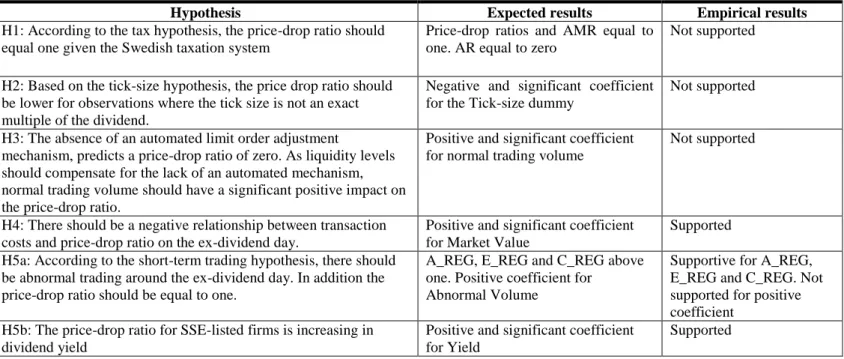
(31) Overall our results show that short-term traders are present around the ex-dividend day. Support for the short-term trading hypothesis is important for three reasons. First, because it implies that short-term traders affect the price-drop ratio. Second, the presence of short-term trading explains why the trading volume increases around the ex-dividend day. Third, it explains why abnormal trading volumes are especially present among high yield stocks, where there are larger net benefits of dividend-capture trading (Karpoff and Walkling, 1990).. 6.3 Summary of results In table 13, we provide a summary of our hypotheses and the empirical results related to each hypotheses.. Table 13 Summary of results The table contains a summary of hypotheses. The empirical results states whether the results from descriptive statistic and regression results supports each hypothesis. Hypothesis Expected results Empirical results H1: According to the tax hypothesis, the price-drop ratio should Price-drop ratios and AMR equal to Not supported equal one given the Swedish taxation system one. AR equal to zero H2: Based on the tick-size hypothesis, the price drop ratio should be lower for observations where the tick size is not an exact multiple of the dividend. H3: The absence of an automated limit order adjustment mechanism, predicts a price-drop ratio of zero. As liquidity levels should compensate for the lack of an automated mechanism, normal trading volume should have a significant positive impact on the price-drop ratio. H4: There should be a negative relationship between transaction costs and price-drop ratio on the ex-dividend day. H5a: According to the short-term trading hypothesis, there should be abnormal trading around the ex-dividend day. In addition the price-drop ratio should be equal to one.. Negative and significant coefficient for the Tick-size dummy. Not supported. Positive and significant coefficient for normal trading volume. Not supported. Positive and significant coefficient for Market Value A_REG, E_REG and C_REG above one. Positive coefficient for Abnormal Volume. Supported. H5b: The price-drop ratio for SSE-listed firms is increasing in dividend yield. Positive and significant coefficient for Yield. Supportive for A_REG, E_REG and C_REG. Not supported for positive coefficient Supported. 30.

(32) 7. Robustness In the regression analysis, we test multiple versions and specifications of the model. This enable a full analysis of the data and the single variables. By doing this, a certain level of robustness is provided to the obtained results. The regression is first done with ordinary least square (OLS). This gives us a first insight of the variables and their relation. However, OLS can provide problems, such as suffering from heteroscedasticity. The first initial tests (both graphical and statistical) could not rule out the absence of heteroscedasticity. In table 14, results from the heteroscedasticity test of the regression model is presented.. Table 14 Heteroscedasticity test Breusch-Pagan / Cook-Weisberg test for heteroscedasticity H0:. Constant variance. Variables:. Fitted values of Price-drop ratio. Chi2(1). =. 137.86. Prob > chi2. =. 0.0000. As the chi-squared value is large (137.86) we can reject the null hypothesis, constant variance and homoscedasticity, at a 1% significance level. The use of heteroscedasticity consistent standard errors is therefore suitable.. We provide results from models with both Eicker-Huber-White and two-way clustered standard errors in this study. Two-way clustered standard errors are clustered within firms and year. This means that these standard errors allow for heteroscedasticity and autocorrelation within a group, in this case for a specific firm or year. It is logical to assume that heteroscedasticity is present within firms or years. Thus, the unobservables of dividend pay-outs belonging to the same company will be correlated (e.g. dividend strategy, ownership structure) while it will not be correlated with firms in a whole different industry. Clustered standard errors do however treat the errors as uncorrelated across entities. As we cannot be sure of the absence of heteroscedasticity between firms and years, Eicker-Huber-White standard errors (written as “robust se” in this study) are also presented for robustness.. 31.

(33) A couple of values are quite large in absolute numbers. For example, Normal trading volume and Market value. To make the coefficient easier to interpret, market value has been scaled down by 1,000,000 SEK. The smallest market value of our data sample is approximately 60 million, making a scaling of 100,000,000 SEK to large with respect to interpretation. However, as normal trading volume is used to calculate other variables such as A_REG and is therefore not scaled down.. We calculate and compare different specifications of the price-drop ratio to ensure a robust measurement of our dependent variable. We prefer close-to-close price-drop ratio over closeto-open as it include the trading movements on the ex-dividend day. To minimize the effect of extreme outliers, we globally winsorize the price-drop ratio at the 0.5th and 99.5th percentiles.. 8. Conclusion The purpose of this thesis was to find the factors impacting the stock price behaviour on the exdividend day. We find an average price-drop ratio of 72% and 56% in our close-to-close and close-to-open sample, respectively. These results are in line with most previous studies and imply that the stock prices on average drop by less than the value of the dividend on the exdividend day. Even when adjusting for market returns, the stock prices drop by less than the value of the dividend on the ex-dividend day. This finding is inconsistent with the theoretically implied price-drop ratio of one.. We find that there is abnormal trading volume around the ex-dividend day, especially among stocks with high dividend yield. In line with previous studies, we also find a positive relationship between the price-drop ratio and dividend yield. Both these results are consistent with the presence of short-term traders and dividend capturing on the SSE. It seems as if the short-term traders are present and mainly focus on high-yield stocks, since the net benefits from trading in these stocks are larger. The trading activity from these traders forces the price-drop ratio to approach one, resulting in ratios closer to one in high-yield stocks. In addition, the intraday increase in the price-drop ratios indicate that intra-day trading activity to some extent eliminates the price-drop anomaly.. 32.

No results found