The Robustness of Resource Allocation in Parallel and Distributed Computing Systems

The Robustness of Resource Allocation in Parallel

and Distributed Computing Systems

Shoukat Ali

Computer Engineering Rolla, MO 65409–0040 Email: [email protected]

Howard Jay Siegel

and Anthony A. Maciejewski

Colorado State University

‡_{Department of Electrical and Computer Engineering} §_{Department of Computer Science}

Fort Collins, CO 80523–1373 Email:{hj, aam}@colostate.edu

Abstract— This paper gives an overview of the material to be

discussed in the invited keynote presentation by H. J. Siegel; it summarizes our research in [1].

Performing computing and communication tasks on parallel and distributed systems involves the coordinated use of different types of machines, networks, interfaces, and other resources. Decisions about how best to allocate resources are often based on estimated values of task and system parameters, due to uncertainties in the system environment. An important research problem is the development of resource management strategies that can guarantee a particular system performance given such uncertainties. We have designed a methodology for deriving the degree of robustness of a resource allocation - the maximum amount of collective uncertainty in system parameters within which a user-specified level of system performance (QoS) can be guaranteed. Our four-step procedure for deriving a robustness metric for an arbitrary system will be presented. We will illustrate this procedure and its usefulness by deriving robustness metrics for some example distributed systems.

I. INTRODUCTION

This paper gives an overview of the material to be discussed in the invited keynote presentation by H. J. Siegel; it summa-rizes our research in [1].

This research focusses on the robustness of a resource allocation in parallel and distributed computing systems. What does robustness mean? Some dictionary definitions of robust-ness are: (a) strong and healthy, as in “a robust person” or “a robust mind,” (b) sturdy or strongly formed, as in “a robust plastic,” (c) suited to or requiring strength as in “a robust exercise” or “robust work,” (d) firm in purpose or outlook as in “robust faith,” (e) full-bodied as in “robust coffee,” and (f) rough or rude as in “stories laden with robust humor.”

In the context of resource allocation in parallel and dis-tributed computing systems, how is the concept of robustness defined? Parallel and distributed systems may operate in an en-vironment where certain system performance features degrade due to unpredictable circumstances, such as sudden machine failures, higher than expected system load, or inaccuracies in the estimation of system parameters (e.g., [2]–[8]). An

This research was supported by the DARPA/ITO Quorum Program through the Office of Naval Research under Grant No. N00014-00-1-0599, and by the Colorado State University George T. Abell Endowment. Some of the equipment used was donated by Intel and Microsoft.

important question then arises: given a system design, what extent of departure from the assumed circumstances will cause a performance feature to be unacceptably degraded? That is, how robust is the system? Before answering this question one needs to clearly define robustness.

In the realm of distributed systems, robustness has been defined in different ways by different researchers. According to [6], robustness is the degree to which a system can function correctly in the presence of inputs different from those assumed. In a more general sense, [4] states that a robust system continues to operate correctly across a wide range of operational conditions. Robustness, according to [5], guarantees the maintenance of certain desired system charac-teristics despite fluctuations in the behavior of its component parts or its environment. The concept of robustness, as used in this research, is similar to that in [5]. Like [5], this work emphasizes that robustness should be defined for a given set of system features, with a given set of perturbations applied to the system. This research investigates the robustness of resource allocation in parallel and distributed systems, and accordingly customizes the definition of robustness.

This paper argues that any claim of robustness for a given system should be followed by three items of information: (a) what behavior of the system makes it robust? (b) what uncertainties is the system robust against? (c) quantitatively, exactly how robust is the system? In this paper, we want to know what robustness means in the context of resource allocation. How is it quantified? How is it measured? Why does it matter?

A resource allocation is defined to be robust with respect to specified system performance features against perturbations in specified system parameters if degradation in these features is limited when the perturbations occur. For example, if a resource allocation has been declared to be robust with respect to satisfying a throughput requirement against perturbations in the system load, then the system, configured under that allocation, should continue to operate without a throughput violation when the system load increases. The immediate question is: what is the degree of robustness? That is, for the example given above, how much can the system load increase before a throughput violation occurs? This research 0-7695-2210-6/04 $20.00 © 2004

addresses this question, and others related to it, by formulating the mathematical description of a metric that evaluates the robustness of a resource allocation with respect to certain system performance features against multiple perturbations in multiple system components and environmental conditions. In addition, this work outlines a procedure called FePIA (named after the four steps that constitute the procedure) for deriving a robustness metric for an arbitrary system. For illustration, the procedure is employed to derive robustness metrics for two example distributed systems. The robustness metric and the FePIA procedure for its derivation are the main contributions of this paper.

The rest of the paper is organized as follows. Section II describes the FePIA procedure mentioned above. It also defines a generalized robustness metric. Derivations of this metric for two example parallel and distributed systems are given in Section III. Section IV presents some experiments that highlight the usefulness of the robustness metric. Section VI outlines some future work, and Section VII concludes the paper.

II. GENERALIZEDROBUSTNESSMETRIC

This section presents a general procedure, called FePIA, for deriving a general robustness metric for any desired computing environment. The name for the above procedure stands for identifying the performance features, the perturbation param-eters, the impact of perturbation parameters on performance features, and the analysis to determine the robustness. Specific examples illustrating the application of the FePIA procedure to sample systems are given in the next section. Each step of the FePIA procedure is now described.

1) Describe quantitatively the requirement that makes the system robust. Based on this robustness requirement, deter-mine the QoS performance features that should be limited in variation to ensure that the robustness requirement is met. Identify the acceptable variation for these feature values as a result of uncertainties in system parameters. Consider an example where (a) the QoS performance feature is makespan (the total time it takes to complete the execution of a set of applications) for a given resource allocation, (b) the acceptable variation is up to a 30% increase of the makespan that was calculated for the given resource allocation using estimated execution times of applications on the machines they are assigned, and (c) the uncertainties in system parameters are inaccuracies in the estimates of these execution times.

Mathematically, let Φ be the set of system performance features that should be limited in variation. For each element

φi ∈ Φ, quantitatively describe the tolerable variation inφi. Let Dβmin

i , βimax

E

be a tuple that gives the bounds of the tolerable variation in the system featureφi. For the makespan example, φi is the time thei-th machine finishes its assigned applications, and its corresponding

βmin i , βmaxi

could be h0, 1.3×(estimated makespan value)i.

2) Identify all of the system and environment parameters whose values may impact the QoS performance features se-lected in step 1. These are called the perturbation parameters

(these are similar to hazards in [3]), and the performance features are required to be robust with respect to these per-turbation parameters. For the makespan example above, the resource allocation (and its associated estimated makespan) was based on the estimated application execution times. It is desired that the makespan be robust (stay within 130% of its estimated value) with respect to uncertainties in these estimated execution times.

Mathematically, letΠbe the set of perturbation parameters. It is assumed that the elements of Π are vectors. Let πj be the j-th element of Π. For the makespan example, πj could be the vector composed of the actual application execution times, i.e., the i-th element of πj is the actual execution time of the i-th application on the machine it was assigned. In general, representation of the perturbation parameters as separate elements of Π would be based on their nature or kind (e.g., message length variables in π1 and computation time variables inπ2).

3) Identify the impact of the perturbation parameters in step 2 on the system performance features in step 1. For the makespan example, the sum of the actual execution times for all of the applications assigned a given machine is the time when that machine completes its applications. Note that 1(b) implies that the actual time each machine finishes its applications must be within the acceptable variation.

Mathematically, for every φi ∈ Φ, determine the relation-ship φi = fij(πj), if any, that relates φi to πj. In this expression, fij is a function that maps πj to φi. For the makespan example,φi is the finishing time for machine mi, andfij would be the sum of execution times for applications assigned to machine mi. The rest of this discussion will be developed assuming only one element in Π. The case where multiple perturbation parameters can affect a given φi simultaneously is examined in [1].

4) The last step is to determine the smallest collective variation in the values of perturbation parameters identified in step 2 that will cause any of the performance features identified in step 1 to violate its acceptable variation. This will be the degree of robustness of the given resource allocation. For the makespan example, this will be some quantification of the total amount of inaccuracy in the execution times estimates allowable before the actual makespan exceeds 130% of its estimated value.

Mathematically, for every φi∈Φ, determine the boundary values ofπj, i.e., the values satisfying the boundary relation-shipsfij(πj) =βiminandfij(πj) =βimax. (Ifπjis a discrete variable then the boundary values correspond to the closest values that bracket each boundary relationship. See [1] for an example.) These relationships separate the region of robust operation from that of non-robust operation. Find the smallest perturbation inπjthat causes anyφi∈Φto exceed the bounds

βmin i , βimax

imposed on it by the robustness requirement. Specifically, letπ_jorigbe the value ofπjat which the system is originally assumed to operate. However, due to inaccuracies in the estimated parameters or changes in the environment, the value of the variableπj might differ from its assumed value.

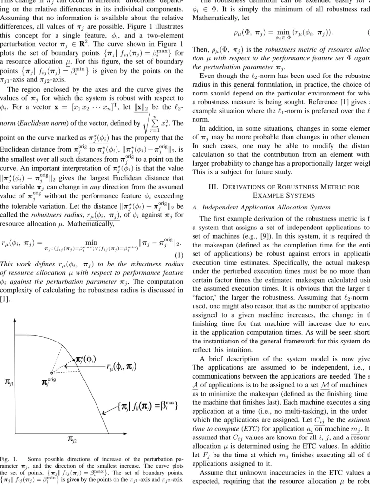
This change inπj can occur in different “directions” depend-ing on the relative differences in its individual components. Assuming that no information is available about the relative differences, all values of πj are possible. Figure 1 illustrates this concept for a single feature, φi, and a two-element perturbation vector πj ∈ R2. The curve shown in Figure 1 plots the set of boundary points {πj||fij(πj) =βimax} for a resource allocation µ. For this figure, the set of boundary points

πj||fij(πj) =βimin is given by the points on the

πj1-axis andπj2-axis.

The region enclosed by the axes and the curve gives the values of πj for which the system is robust with respect to

φi. For a vector x = [x1x2· · · xn]T, let kxk2 be the ` 2-norm (Euclidean 2-norm) of the vector, defined by

s n P r=1 x2 r. The point on the curve marked asπ?

j(φi)has the property that the Euclidean distance fromπ_jorigtoπ?

j(φi),kπ?j(φi)−π orig j k2, is the smallest over all such distances fromπ_jorigto a point on the curve. An important interpretation ofπ?_j(φi)is that the value kπ?

j(φi)−π orig

j k2 gives the largest Euclidean distance that the variableπj can change in any direction from the assumed value of π_jorig without the performance feature φi exceeding the tolerable variation. Let the distancekπ?_j(φi)−π_jorigk2 be called the robustness radius, rµ(φi, πj), ofφi againstπj for resource allocationµ. Mathematically,

rµ(φi, πj) = min

πj: (fij(πj)=βmaxi )∨(fij(πj)=βmini )

kπj−πorigj k2. (1) This work defines rµ(φi, πj) to be the robustness radius of resource allocation µ with respect to performance feature

φi against the perturbation parameter πj. The computation complexity of calculating the robustness radius is discussed in [1].

λ

ππ

ππ

(φi)

r

(φi, j)

ππ

|

f

(

ππ

) =

{ππ

β

}

πj

πj

Fig. 1. Some possible directions of increase of the perturbation pa-rameter πj, and the direction of the smallest increase. The curve plots the set of points,

πj||fij(πj) =βimax . The set of boundary points,

πj||fij(πj) =βimin is given by the points on theπj1-axis andπj2-axis.

The robustness definition can be extended easily for all

φi ∈ Φ. It is simply the minimum of all robustness radii. Mathematically, let

ρµ(Φ, πj) = min φi∈Φ

(rµ(φi, πj)). (2) Then, ρµ(Φ, πj)is the robustness metric of resource alloca-tion µ with respect to the performance feature setΦ against the perturbation parameterπj.

Even though the`2-norm has been used for the robustness radius in this general formulation, in practice, the choice of a norm should depend on the particular environment for which a robustness measure is being sought. Reference [1] gives an example situation where the`1-norm is preferred over the` 2-norm.

In addition, in some situations, changes in some elements of πj may be more probable than changes in other elements. In such cases, one may be able to modify the distance calculation so that the contribution from an element with a larger probability to change has a proportionally larger weight. This is a subject for future study.

III. DERIVATIONS OFROBUSTNESSMETRIC FOR

EXAMPLESYSTEMS

A. Independent Application Allocation System

The first example derivation of the robustness metric is for a system that assigns a set of independent applications to a set of machines (e.g., [9]). In this system, it is required that the makespan (defined as the completion time for the entire set of applications) be robust against errors in application execution time estimates. Specifically, the actual makespan under the perturbed execution times must be no more than a certain factor times the estimated makespan calculated using the assumed execution times. It is obvious that the larger the “factor,” the larger the robustness. Assuming that`2-norm is used, one might also reason that as the number of applications assigned to a given machine increases, the change in the finishing time for that machine will increase due to errors in the application computation times. As will be seen shortly, the instantiation of the general framework for this system does reflect this intuition.

A brief description of the system model is now given. The applications are assumed to be independent, i.e., no communications between the applications are needed. The set Aof applications is to be assigned to a setMof machines so as to minimize the makespan (defined as the finishing time of the machine that finishes last). Each machine executes a single application at a time (i.e., no multi-tasking), in the order in which the applications are assigned. LetCij be the estimated time to compute (ETC) for applicationaion machinemj. It is assumed thatCij values are known for alli,j, and a resource allocationµis determined using the ETC values. In addition, let Fj be the time at which mj finishes executing all of the applications assigned to it.

Assume that unknown inaccuracies in the ETC values are expected, requiring that the resource allocation µ be robust

against them. More specifically, it is required that, for a given resource allocation, its actual makespan value M (calculated considering the effects of ETC errors) may be no more than

τ times its estimated value,Mest_{. The estimated value of the}

makespan is the value calculated assuming the estimated ETC values. Following step 1 of the FePIA procedure in Section II, the system performance features that should be limited in variation to ensure the makespan robustness are the finishing times of the machines. That is,Φ ={Fj|| 1≤j≤ |M|}.

According to step 2 of the FePIA procedure, the pertur-bation parameter needs to be defined. Let Cest

i be the ETC value for applicationai on the machine where it is assigned. Let Ci be equal to the actual computation time value (Ciest plus the estimation error). In addition, let C be the vector of the Ci values, such that C = [C1 C2 · · · C|A|]. Similarly, Cest_{= [C}est

1 C2est · · · C|A|est]. The vectorC is the perturbation parameter for this analysis.

In accordance with step 3 of the FePIA procedure, Fj has to be expressed as a function of C. To that end,

Fj(C) =

X

i:aiis assigned tomj

Ci. (3)

Note that the finishing time of a given machine depends only on the actual execution times of the applications as-signed to that machine, and is independent of the finish-ing times of the other machines. Followfinish-ing step 4 of the FePIA procedure, the set of boundary relationships corre-sponding to the set of performance features is given by {Fj(C) =τ Mest_{|| 1≤j≤ |M|}.}

For a two-application system,Ccorresponds toπjin Figure 1. Similarly, C1 and C2 correspond to πj1 and πj2, respec-tively. The termsCest_{,Fj(C), andτ M}est_{correspond toπ}orig

j ,

fij(πj), and βimax, respectively. The boundary relationship “Fj(C) = τ Mest_{” corresponds to the boundary relationship}

“fij(πj) =βimax.”

From Equation 1, the robustness radius of Fj against C is given by

rµ(Fj, C) = min C:Fj(C)=τ Mest

kC−Cestk2 (4) That is, if the Euclidean distance between any vector of the actual execution times and the vector of the estimated execution times is no larger thanrµ(Fj, C), then the finishing time of machine mj will be at most τ times the estimated makespan value.

Note that the right hand side in Equation 4 can be interpreted as the perpendicular distance from the point Cest to the hyperplane described by the equation τ Mest−Fj(C) = 0. Using the point-to-plane distance formula [10], Equation 4 reduces to

rµ(Fj, C) =

τ Mest_−F j(Cest)

p

number of applications assigned to mj (5) The robustness metric, from Equation 2, is ρµ(Φ, C) = minF_j∈Φrµ(Fj, C). That is, if the Euclidean distance be-tween any vector of the actual execution times and the vector

of the estimated execution times is no larger than ρµ(Φ, C), then the actual makespan will be at mostτ times the estimated makespan value. The value ofρµ(Φ, C)has the units of C, namely time.

B. The HiPer-D System

The second example derivation of the robustness metric is for a HiPer-D [11] like system that assigns a set of continuously executing, communicating applications to a set of machines. It is required that the system be robust with respect to certain QoS attributes against unforeseen increases in the “system load.”

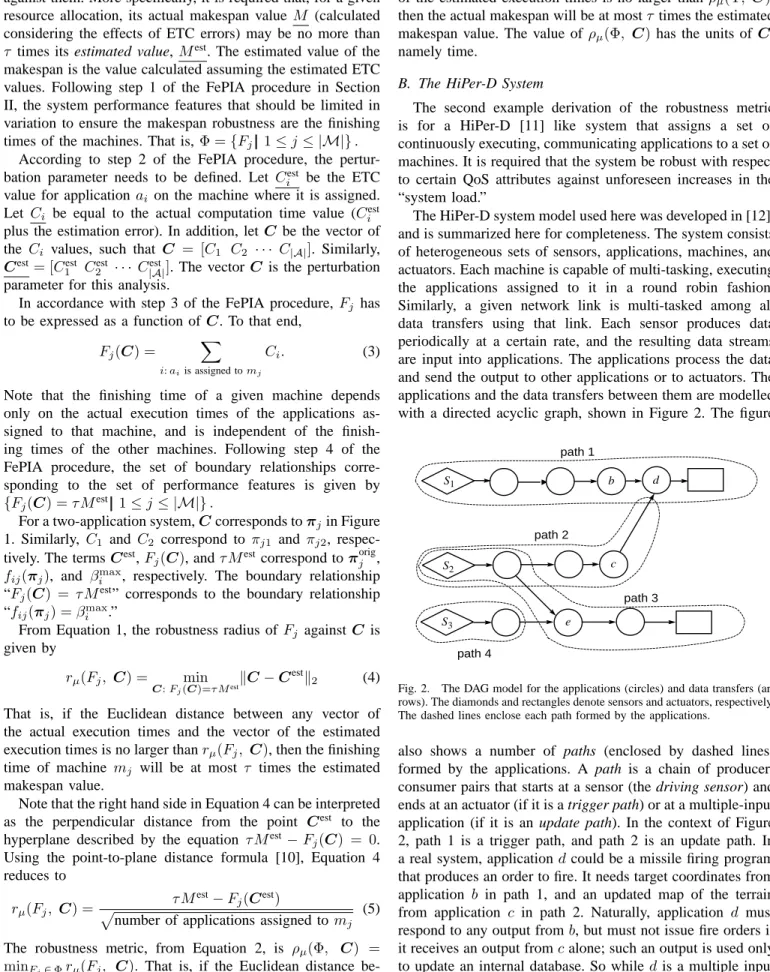
The HiPer-D system model used here was developed in [12], and is summarized here for completeness. The system consists of heterogeneous sets of sensors, applications, machines, and actuators. Each machine is capable of multi-tasking, executing the applications assigned to it in a round robin fashion. Similarly, a given network link is multi-tasked among all data transfers using that link. Each sensor produces data periodically at a certain rate, and the resulting data streams are input into applications. The applications process the data and send the output to other applications or to actuators. The applications and the data transfers between them are modelled with a directed acyclic graph, shown in Figure 2. The figure

path 1 path 2 path 3 path 4 S1 S2 S3 d e b c

Fig. 2. The DAG model for the applications (circles) and data transfers (ar-rows). The diamonds and rectangles denote sensors and actuators, respectively. The dashed lines enclose each path formed by the applications.

also shows a number of paths (enclosed by dashed lines) formed by the applications. A path is a chain of producer-consumer pairs that starts at a sensor (the driving sensor) and ends at an actuator (if it is a trigger path) or at a multiple-input application (if it is an update path). In the context of Figure 2, path 1 is a trigger path, and path 2 is an update path. In a real system, applicationdcould be a missile firing program that produces an order to fire. It needs target coordinates from application b in path 1, and an updated map of the terrain from application c in path 2. Naturally, application d must respond to any output fromb, but must not issue fire orders if it receives an output fromcalone; such an output is used only to update an internal database. So whiledis a multiple input application, the rate at which it produces data is equal to the

rate at which the trigger application b produces data (in the HiPer-D model). That rate, in turn, equals the rate at which the driving sensor, S1, produces data. The problem specification indicates the path to which each application belongs, and the corresponding driving sensor.

Let P be the set of all paths, andPk be the list of appli-cations that belong to the k-th path. Note that an application may be present in multiple paths. As in Subsection III-A, A is the set of applications.

The sensors constitute the input interface of the system to the external world. Let the maximum periodic data output rate from a given sensor be called its output data rate. The minimum throughput constraint states that the computation or communication time of any application in Pk is required to be no larger than the reciprocal of the output data rate of the driving sensor for Pk. For application ai ∈ Pk, let R(ai) be set to the output data rate of the driving sensor for Pk. In addition, let T_ijc be the computation time for applicationai assigned to machinemj. Also, letTipn be the time to send data from application ai to application ap. Because this analysis is being carried out for a specific resource allocation, the machine where a given application is assigned is known. It is assumed thatai is assigned tomj, and the machine subscript forT_ijc is omitted in the ensuing analysis for clarity unless the intent is to show the relationship between execution times of

ai at various possible machines.

The maximum end-to-end latency constraint states that, for a given pathPk, the time taken between the instant the driving sensor outputs a data set until the instant the actuator or the multiple-input application fed by the path receives the result of the computation on that data set must be no greater than a given value, Lmax

k . Let Lk be the actual (as opposed to the maximum allowed) value of the end-to-end latency for Pk. The quantityLk can be found by adding the computation and communication times for all applications inPk (including any sensor or actuator communications). Let D(ai) be the set of successor applications of ai. Then,

Lk= X i:ai∈Pk p: (ap∈Pk)∧(ap∈D(ai)) T_ic + T_ipn . (6)

It is desired that a given resource allocationµof the system be robust with respect to the satisfaction of two QoS attributes: the latency and throughput constraints. Following step 1 of the FePIA procedure in Section II, the system performance features that should be limited in variation are the latency values for the paths and the computation and communication time values for the applications. The set Φis given by

Φ ={T_ic|| 1≤i≤ |A|}

[

T_ipn||(1≤i≤ |A|)∧(for pwhereap∈ D(ai))

[

Lk||1≤k≤ |P| (7)

This system is expected to operate under uncertain outputs from the sensors, requiring that the resource allocation µ be robust against unpredictable workload increases in the sensor

outputs. Let λz be the workload output from thez-th sensor in the set of sensors, and be defined as the number of objects present in the most recent data set from that sensor. The system workload,λ, is the vector composed of the load values from all sensors. Letλinit _{be the initial value ofλ, and λ}init

i be the initial value of thei-th member ofλinit_{. Following step 2, the}

perturbation parameterπj is identified to beλ.

Step 3 of the FePIA procedure requires that the impact of λ on each of the system performance features be identified. The computation times of different applications (and the communication times of different data transfers) are likely to be of different complexities with respect toλ. Assume that the dependence ofTc

i andTipn onλis known (or can be estimated) for all i, p. Given that, Tc

i and Tipn can be re-expressed as functions ofλ asTc

i(λ)andTipn(λ), respectively. In general,

Tc

i(λ)andTipn(λ)will be functions of the loads from all those sensors that can be traced back from ai. For example, the computation time for application din Figure 2 is a function of the loads from sensorsS1 andS2, but that for application

e is a function ofS2 andS3 loads (but each application has just one driving sensor:S1fordandS2fore). Then Equation 6 can be used to expressLk as a function ofλ.

Following step 4 of the FePIA procedure, the set of bound-ary relationships corresponding to Equation 7 is given by

{Tic(λ) = 1/R(ai)||1≤i≤ |A|}

[

Tipn(λ) = 1/R(ai)||(1≤i≤ |A|)∧(forpwhereap∈ D(ai))

[

Lk(λ) =Lmaxk ||1≤k≤ |P|}.

Then, using Equation 1, one can find, for each φi ∈ Φ, the robustness radius,rµ(φi, λ). Specifically,

rµ(φi, λ) =              min λ:Tc x(λ)=1/R(ax) kλ−λinitk2 ifφi=Txc (8a) min λ:Tn xy(λ)=1/R(ax) kλ−λinitk2 ifφi=Txyn (8b) min λ:Lk(λ)=Lmaxk kλ−λinitk2 ifφi=Lk (8c)

The robustness radius in Equation 8a is the largest increase (Euclidean distance) in load in any direction (i.e., for any combination of sensor load values) from the assumed value that does not cause a throughput violation for the computation of applicationax. This is because it corresponds to the value of λ for which the computation time of ax will be at the allowed limit of 1/R(ax). The robustness radii in Equations 8b and 8c are the similar values for the communications of application ax and the latency of path Pk, respectively. The robustness metric, from Equation 2, is given by ρµ(Φ, λ) = minφi∈Φ(rµ(φi, λ)). For this system, ρµ(Φ, λ) is the largest increase in load in any direction from the assumed value that does not cause a latency or throughput violation for any application or path. Note thatρµ(Φ, λ)has the units ofλ, namely objects per data set. In addition, note that althoughλis a discrete variable, it has been treated as a continuous variable in Equation 8 for the purpose of simplifying the illustration. A method for handling a discrete perturbation parameter is discussed in [1].

IV. EXPERIMENTS

The experiments in this section seek to establish the utility of the robustness metric in distinguishing between resource allocations that perform similarly in terms of a commonly used metric, such as makespan. Two different systems were considered: the independent task allocation system discussed in Subsection III-A and the HiPer-D system outlined in Sub-section III-B. Experiments were performed for a system with five machines and 20 applications. A total of 1000 resource allocations were generated by assigning a randomly chosen machine to each application, and then each resource allocation was evaluated with the robustness metric and the commonly used metric.

Independent Application Allocation System: For the system

in Subsection III-A, the ETC values were generated by sam-pling a Gamma distribution. The mean was arbitrarily set to 10, the task heterogeneity was set to 0.7, and the machine heterogeneity was also set to 0.7 (the heterogeneity of a set of numbers is the standard deviation divided by the mean). See [13] for a description of a method for generating random numbers with given mean and heterogeneity values.

The resource allocations were evaluated for robustness, makespan, and load balance index (defined as the ratio of the finishing time of the machine that finishes first to the makespan). The larger the value of the load balance index, the more balanced the load (the largest value being 1). The tolerance,τ, was set to 120% (i.e., the actual makespan could be no more than 1.2 times the estimated value). In this context, a robustness value ofxfor a given resource allocation means that the resource allocation can endure any combination of ETC errors without the makespan increasing beyond 1.2 times its estimated value as long as the Euclidean norm of the errors is no larger than xseconds.

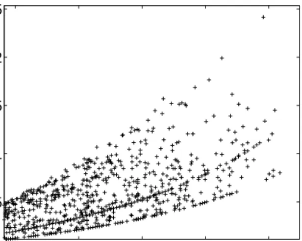
Figure 3(a) shows the “normalized robustness” of a re-source allocation against its makespan. The normalized robust-ness equals the absolute robustrobust-ness divided by the estimated makespan. A similar graph for the normalized robustness against the load balance index is shown in Figure 3(b). It can be seen in Figure 3 that some resource allocations are clustered into groups, such that for all resource allocations within a group, the normalized robustness remains constant as the estimated makespan (or load balance index) increases.

The cluster of the resource allocations with the highest robustness has the feature that the most loaded machine has the smallest number of applications assigned to it (which is two for the experiments in Figure 3). The cluster with the smallest robustness has the largest number, 11, of applications assigned to it. The intuitive explanation for this behavior is that the larger the number of applications assigned to a machine, the more degrees of freedom for the finishing time of that machine. A larger degree of freedom then results in a shorter path to constraint violation in the parameter space. That is, the robustness is then smaller (using the`2-norm). The formal explanation is given in [1].

If one agrees with the utility of the observations made

above, one can still question if the same information could be gleaned from some traditional metrics (even if they are not traditionally used to measure robustness). In an attempt to answer that question, note that sharp differences exist in the robustness of some resource allocations that have very similar values of makespan. A similar observation could be made from the robustness against load balance index plot (Figure 3(b)). In fact, it is possible to find a set of resource allocations that have very similar values of makespan, and very similar values of load balance index, but with very different values of the robustness. These observations highlight the fact that the information given by the robustness metric could not be obtained from two popular performance metrics.

40 60 80 100 120 0.07 0.08 0.09 0.1 0.11 0.12 0.13 0.14 makespan (seconds) normalized robustness (a) 0 0.2 0.4 0.6 0.8 0.07 0.08 0.09 0.1 0.11 0.12 0.13 0.14

load balance index

normalized robustness

(b)

Fig. 3. The plots of normalized robustness against (a) makespan, and (b) load balance index for 1000 randomly generated resource allocations

The HiPer-D System: For the model in Subsection III-B,

the experiments were performed for a system that consisted of 19 paths, where the end-to-end latency constraints of the

paths were uniformly sampled from the range [750, 1250]. The system had three sensors (with rates 4 × 10−5_{,3 ×} 10−5_{, and 8×10}−6_{), and three actuators. The experiments} made the following simplifying assumptions. The computa-tion time funccomputa-tion, Tc

ij(λ), was assumed to be of the form

P

1≤z≤3bijzλz, wherebijz = 0if there is no route from the

z-th sensor to application ai. Otherwise, bijz was sampled from a Gamma distribution with a mean of 10 and task and machine heterogeneity values of 0.7 each. For simplicity in the presentation of the results, the communication times were all set to zero. These assumptions were made only to simplify the experiments, and are not a part of the formulation of the robustness metric. The salient point in this example is that the utility of the robustness metric can be seen even when simple complexity functions are used.

The resource allocations were evaluated for robustness and “slack.” In this context, a robustness value of x for a given resource allocation means that the resource allocation can endure any combination of sensor loads without a latency or throughput violation as long as the Euclidean norm of the increases in sensor loads (from the initial values) is no larger thanx. Slack has been used in many studies as a performance measure (e.g., [6], [14]) for resource allocation in parallel and distributed systems, where a resource allocation with a larger slack is considered better. In this study, slack is defined mathematically as follows. Let the fractional value of a given QoS attribute be the value of the attribute as a percentage of the maximum allowed value. Then the percentage slack for a given QoS attribute is the fractional value subtracted from 1. The system-wide percentage slack is the minimum value of percentage slack taken over all QoS constraints, and can be expressed mathematically as min min k:P_k∈P 1−Lk(λ) Lmax k , min i:ai∈A     1− max Tic(λ), max ap∈D(ai) Tipn(λ) 1/R(ai)         . (9)

Figure 4 shows the normalized robustness of a resource allocation against its slack. For this system, the normalized robustness equals the absolute robustness divided by kλinit_k2.

It can be seen that the normalized robustness and slack are not correlated. If, in some research study, the purpose of using slack is to measure a system’s ability to tolerate additional load, then our measure of robustness is a better indicator of that ability than slack. This is because the expression for slack, Equation 9, does not directly take into account how the sensor loads affect the computation and communication times. It could be conjectured that for a system where all sensors affected the computation and communication times of all ap-plications in exactly the same way, the slack and this research’s measure of robustness would be tightly correlated. This, in fact, is true. Other experiments performed in this study show that for a system with small heterogeneity, the robustness and slack are tightly correlated, thereby suggesting that robustness

0.2 0.3 0.4 0.5 0.6 0.5 1 1.5 2 2.5 slack normalized robustness

Fig. 4. The plot of normalized robustness against slack for 1000 randomly generated resource allocations

measurements are not needed if slack is known. As the system heterogeneity increases, the robustness and slack become less correlated, indicating that the robustness measurements can be used to distinguish between resource allocations that are similar in terms of the slack. As the system size increases, the correlation between the slack and the robustness decreases even further. In summary, for heterogeneous systems, using slack as a measure of how much increase in sensor load a system can tolerate may cause system designers to grossly misjudge the system’s capability.

V. RELATEDWORK

Although a number of robustness measures have been studied in the literature (e.g., [3], [6]–[8], [14]–[18]), those measures were developed for specific systems. The focus of the research in this paper is a general mathematical formula-tion of a robustness metric that could be applied to a variety of parallel and distributed systems by following the FePIA procedure presented in this paper.

Given an allocation of a set of communicating applications to a set of machines, the work in [3] develops a metric for the robustness of the makespan against uncertainties in the estimated execution times of the applications. The paper discusses in detail the effect of these uncertainties on the value of makespan, and how the robustness metric could be used to find more robust resource allocations. Based on the model and assumptions in [3], several theorems about the properties of robustness are proven. The robustness metric in [3] was formulated for errors in the estimation of application execution times, and was not intended for general use (in contrast to our work). Additionally, the formulation in [3] assumes that the execution time for any application is at most ktimes the estimated value, wherek≥1 is the same for all applications. In our work, no such bound is assumed.

In [15], the authors address the issue of probabilistic guar-antees for fault-tolerant real-time systems. As a first step

towards determining such a probabilistic guarantee, the authors determine the maximum frequency of software or hardware faults that the system can tolerate without violating any hard real-time constraint. In the second step, the authors derive a value for the probability that the system will not experience faults at a frequency larger than that determined in the first step. The output of the first step is what our work would identify as the robustness of the system, with the satisfaction of the real-time constraints being the robustness requirement, and the occurrence of faults being the perturbation parameter. The research in [16] considers a single-machine scheduling environment where the processing times of individual jobs are uncertain. The system performance is measured by the total flow time (i.e., the sum of completion times of all jobs). Given the probabilistic information about the processing time for each job, the authors determine the normal distribution that approximates the flow time associated with a given schedule. A given schedule’s robustness is then given by 1 minus the risk of achieving substandard flow time performance. The risk value is calculated by using the approximate distribution of flow time.

The studies in [14] and [17] explore slack-based techniques for producing robust resource allocations. While [14] focusses on a job-shop environment, [17] focusses on real-time systems. The central idea is to provide each task with extra time (defined as slack) to execute so that some level of uncertainty can be absorbed without having to reallocate.

In [6], a “neighborhood-based” measure of robustness is defined for a job-shop environment. Given a schedule s and a performance metric P(s), the robustness of the schedule

s is defined to be a weighted sum of all P(s0) values such that s0 is in the set of schedules that can be obtained from

s by interchanging two consecutive operations on the same machine.

The work in [7] develops a mathematical definition for the robustness of makespan against machine breakdowns in a job-shop environment. The authors assume a certain random distri-bution of the machine breakdowns and a certain rescheduling policy in the event of a breakdown. Given these assumptions, the robustness of a schedule s is defined to be a weighted sum of the expected value of the makespan of the rescheduled system, M, and the expected value of the schedule delay (the difference betweenM and the original value of the makespan). Because the analytical determination of the schedule delay be-comes very hard when more than one disruption is considered, the authors propose surrogate measures of robustness that are claimed to be strongly correlated with the expected value of

M and the expected schedule delay.

The research in [8] uses a genetic algorithm to produce robust schedules in a job-shop environment. Given a schedule

sand a performance metricP(s), the “robust fitness value” of the schedulesis a weighted average of allP(s0)values such that s0 is in a set of schedules obtained from s by adding a small “noise” to it. The size of this set of schedules is determined arbitrarily. The “noise” modifies s by randomly changing the ready times of a fraction of the tasks.

Our work is perhaps closest in philosophy to [18], which attempts to calculate the stability radius of an optimal schedule in a job-shop environment. The stability radius of an optimal schedule, s, is defined to be the radius of a closed ball in the space of the numerical input data such that within that ball the schedule s remains optimal. Outside this ball, which is centered at the assumed input, some other schedule would outperform the schedule that is optimal at the assumed input. From our viewpoint, for a given optimal schedule, the robustness requirement could be the persistence of optimality in the face of perturbations in the input data. Our work differs and is more general because we consider the given system requirements to generate a robustness requirement, and then determine the robustness. In addition, our work considers the possibility of multiple perturbations in different dimensions.

VI. FUTUREWORK

We are considering extending our current work in many different directions. Some of these directions include:

1) Incorporating robustness into static (off-line) and dy-namic (on-line) resource allocation heuristics [19]. 2) Deriving the boundary curves for different problem

domains.

3) Incorporating multiple types of perturbation parameters, e.g., sensor loads and estimated execution times. Chal-lenges here are how to define the collective impact to find robust radius and how to state the combined bound on multiple perturbation parameters to maintain the promised performance.

4) Incorporating probabilistic information about uncertain-ties. Such information might be available about individ-ual perturbation parameter elements or one might only have only relative information about perturbation param-eter elements. In another case, one might have relative information about different perturbation parameters. 5) Determining when to use Euclidean distance versus a

simple sum when calculating the collective impact of changes in the perturbation parameter elements.

VII. CONCLUSIONS

This paper argues that any claim of robustness for a given system should be followed by three items of information: (a) what behavior of the system makes it robust? (b) what uncertainties is the system robust against? (c) quantitatively, exactly how robust is the system? The paper presents a mathematical description of a metric for the robustness of a resource allocation with respect to desired system performance features against multiple perturbations in various system and environmental conditions. In addition, the research describes a procedure, called FePIA, to methodically derive the robust-ness metric for a variety of parallel and distributed resource allocation systems. For illustration, the FePIA procedure is employed to derive robustness metrics for two example dis-tributed systems. The experiments conducted illustrate the utility of the robustness metric in distinguishing between resource allocations that perform similarly otherwise.

REFERENCES

[1] S. Ali, A. A. Maciejewski, H. J. Siegel, and J.-K. Kim, “Measuring the robustness of a resource allocation,” IEEE Transactions on Parallel and

Distributed Systems, vol. 15, no. 7, pp. 630–641, July 2004.

[2] P. M. Berry, “Uncertainty in scheduling: probability, problem reduction, abstractions and the user,” IEE Computing and Control Division Collo-quium on Advanced Software Technologies for Scheduling, Digest No. 1993/163, Apr. 26, 1993.

[3] L. B¨ol¨oni and D. C. Marinescu, “Robust scheduling of metaprograms,”

Journal of Scheduling, vol. 5, no. 5, pp. 395–412, Sept. 2002.

[4] S. D. Gribble, “Robustness in complex systems,” in 8th Workshop on

Hot Topics in Operating Systems (HotOS-VIII), May 2001, pp. 21–26.

[5] E. Jen, “Stable or robust? What is the difference?” Complexity, to appear. [6] M. Jensen, “Improving robustness and flexibility of tardiness and total flowtime job shops using robustness measures,” Journal of Applied Soft

Computing, vol. 1, no. 1, pp. 35–52, June 2001.

[7] V. J. Leon, S. D. Wu, and R. H. Storer, “Robustness measures and robust scheduling for job shops,” IEE Transactions, vol. 26, no. 5, pp. 32–43, Sept. 1994.

[8] M. Sevaux and K. S¨orensen, “Genetic algorithm for robust schedules,” in 8th International Workshop on Project Management and Scheduling

(PMS 2002), Apr. 2002, pp. 330–333.

[9] T. D. Braun, H. J. Siegel, N. Beck, L. L. B¨ol¨oni, M. Maheswaran, A. I. Reuther, J. P. Robertson, M. D. Theys, B. Yao, D. Hensgen, and R. F. Freund, “A comparison of eleven static heuristics for mapping a class of independent tasks onto heterogeneous distributed computing systems,”

Journal of Parallel and Distributed Computing, vol. 61, no. 6, pp. 810–

837, June 2001.

[10] G. F. Simmons, Calculus With Analytic Geometry, Second Edition. New York, NY: McGraw-Hill, 1995.

[11] R. Harrison, L. Zitzman, and G. Yoritomo, “High performance dis-tributed computing program (HiPer-D)—engineering testbed one (T1) report,” Naval Surface Warfare Center, Dahlgren, VA, Tech. Rep., Nov. 1995.

[12] S. Ali, J.-K. Kim, Y. Yu, S. B. Gundala, S. Gertphol, H. J. Siegel, A. A. Maciejewski, and V. Prasanna, “Greedy heuristics for resource allocation in dynamic distributed real-time heterogeneous computing systems,” in The 2002 International Conference on Parallel and Distributed

Processing Techniques and Applications (PDPTA 2002), Vol. II, June

2002, pp. 519–530.

[13] S. Ali, H. J. Siegel, M. Maheswaran, D. Hensgen, and S. Sedigh-Ali, “Representing task and machine heterogeneities for heterogeneous computing systems,” Tamkang Journal of Science and Engineering, vol. 3, no. 3, pp. 195–207, invited, Nov. 2000.

[14] A. J. Davenport, C. Gefflot, and J. C. Beck, “Slack-based techniques for robust schedules,” in 6th European Conference on Planning

(ECP-2001), Sept. 2001, pp. 7–18.

[15] A. Burns, S. Punnekkat, B. Littlewood, and D. Wright, “Probabilistic guarantees for fault-tolerant real-time systems,” Design for Validation (DeVa) TR No. 44, Esprit Long Term Research Project No. 20072, Dept. of Computer Science, Univ. of Newcastle upon Tyne, UK, Tech. Rep., 1997.

[16] R. L. Daniels and J. E. Carrillo, “β-Robust scheduling for single-machine systems with uncertain processing times,” IIE Transactions, vol. 29, no. 11, pp. 977–985, 1997.

[17] S. Ghosh, “Guaranteeing Fault Tolerance Through Scheduling in Real-Time Systems,” Ph.D. dissertation, Faculty of Arts and Sciences, Univ. of Pittsburgh, 1996.

[18] Y. N. Sotskov, V. S. Tanaev, and F. Werner, “Stability radius of an optimal schedule: A survey and recent developments,” in Industrial

Applications of Combinatorial Optimization, G. Yu, Ed. Norwell, MA:

Kluwer Academic Publishers, 1998, pp. 72–108.

[19] S. Ali, A. A. Maciejewski, H. J. Siegel, and J.-K. Kim, “Robust resource allocation for distributed computing systems,” in The 2004 International

Conference On Parallel Processing (ICPP 2004), accepted, to appear in