An Analysis of State-Level Economic Impacts from the
Development of Wind Power Plants in Cache County, Utah
Austin Coover Edwin R. Stafford, Ph.D. Cathy L. Hartman, Ph.D.
Center for the Market Diffusion of Renewable Energy and Clean Technology Logan, Utah 84322-3555
This report provides an overview of the state of Utah’s development of its wind resources for the generation of electricity and an economic analysis of potential wind development in Cache County, Utah. This analysis draws on information from local wind developers and utilizes the Jobs and Economic Development Impact (JEDI) model (version W1.10.03) developed by the U.S. Department of Energy’s National Renewable Energy Laboratory (NREL) to estimate the total economic impacts (labor, supply chain, and induced) that could result from the development of a wind power plant in Cache County. Findings detail how a Cache County wind power plant could benefit the state in terms of job
opportunities (during both construction and operations), lease payments to landowners, property tax revenues for local schools and communities, and overall economic output for the state.
The authors thank David Keyser of the Strategic Energy Analysis Center at the National Renewable Energy Laboratory, Golden, CO, for his peer-review and helpful comments on an earlier draft of this report.
1 Introduction
According to the American Wind Energy Association (AWEA), 2012 was another record-breaking year for wind energy development across the United States with the construction of 13,124 megawatts (MW) of new capacity, accounting for 42 percent of all electricity generation built (Reuters 2013). While Texas leads the nation in total wind power capacity of over 12,000 MW, Iowa ranked first in terms of percent of its electricity generated from wind – 24.5 percent. South Dakota ranked second with 23.9 percent of its power coming from wind. To date, seven other states produce more than 10 percent of their
electricity from wind, including North Dakota, Minnesota, Kansas, Colorado, Oklahoma, and Oregon. In total, the United States has over 60,000 MW of wind power capacity, the equivalent of powering 15 million homes (Reuters 2013).
Developers in the United States raced to construct wind projects in 2012 to qualify for the federal Production Tax Credit that was scheduled to expire at the end of year. The Production Tax Credit is an income tax credit of $0.023 per kilowatt hour for the production of electricity from utility-scale wind turbines for a wind project’s first ten years of operation (Del Franco 2013). Despite bipartisan support, Congress allowed the PTC to expire, only to extend it for one year just hours later as part of the
American Taxpayer Relief Act of 2012 on New Year’s Day 2013. Uncertainty over the PTC’s extension, nonetheless, forced many wind development companies, turbine manufacturers, and their supply chains to scale back operations and lay-off workers throughout 2012 over fears of reduced development in 2013 in the absence of tax incentives. Historically, the on-again, off-again nature of the PTC since 2000 has resulted in “boom and bust” cycles for wind energy development, and AWEA and other wind energy advocates are seeking to establish a more stable and predictable energy policy to encourage future market certainty and investment (Gramlich 2013).
Aside from the PTC, other factors have been contributing to wind energy’s rapid development in recent years, including state-level “renewable portfolio standards” (RPS) that mandate utilities to incorporate increasing levels of renewable energy onto their systems (established in 29 states and the District of Columbia) (Del Franco 2012a); technological and supply-chain/production advances that have increased wind turbine power efficiency and decreased costs (Zuhlke 2012); and the desire to exploit wind
energy’s economic benefits, including domestic construction job creation, lease payments to landowners in rural agricultural communities, and wind energy’s inherent price stability and predictability that can be a hedge against volatile fossil fuel costs (Hartman, Stafford, and Reategui 2011).
In addition to PTC uncertainty after 2013, wind energy development faces other obstacles. Current low natural gas prices have made investments in wind (and other energy resources, including fossil fuels and nuclear power) less attractive (Martin 2013a). There is also a political movement underway to repeal state-level RPS legislation, which could threaten future demand for wind energy and other renewable energy sources (Martin 2013b). Additionally, growing citizen resistance to local wind energy
development has also impeded the approval process for many proposed projects (Stafford and Hartman 2012). Indeed, organized opposition has delayed construction of the proposed Cape Wind project off of Cape Cod, Massachusetts, for over 12 years (Mohl 2013). Though organized opposition may be a
2
challenge, proactive developer engagement with the community throughout the development process to accommodate citizen concerns and demonstrate the value of local wind development (e.g., increased property tax revenues for local schools and services, creation of jobs, environmental benefits, etc.) can often lead to resolution of differences (see Stafford and Hartman 2012).
In the face of volatile energy prices, supply uncertainties, and the desire to generate more energy from domestic resources, wind energy is increasingly recognized as a cost-effective energy resource that can diversify America’s current energy resources and not contribute to climate change or result in major adverse environmental impacts (e.g., carbon and sulfur emissions, nuclear waste, water consumption). In May 2008, the U.S. Department of Energy issued a report declaring that wind power was capable of becoming a major contributor to America’s electricity supply over the next three decades, setting a vision that wind energy could contribute to 20 percent of America’s electricity generation (U.S.
Department of Energy 2008). The report outlines various key barriers that must be overcome to reach 20 percent, including uniform policies across regions, investments in transmission, accommodation of wind energy’s variability onto the grid, siting projects that are compatible with local communities and wildlife, building up of the supply chain for wind turbine manufactures, and advancing turbine
performance and efficiency. The American Wind Energy Association has been working to address these issues to facilitate the industry’s growth and public acceptance.
Utah’s Wind Development
In 2009, the Utah Renewable Energy Zone (UREZ) Task Force (appointed by Governor Jon Huntsman, Jr.) published a report identifying suitable locations for the development of wind, solar, and geothermal technologies in large quantities and at competitive energy market prices (Barry et al. 2009). The UREZ Task Force estimated that the state of Utah could generate over 9,000 MW from 51 potential wind locations.
As of June 2013, the state of Utah had approximately 325 MW of wind power capacity derived from two commercial wind projects. Utah’s first commercial wind power plant, situated at the mouth of Spanish Fork Canyon in Utah County, commenced operations in June 2008. Developed by Wasatch Wind and Edison Mission Energy, a Utah State University/U.S. Department of Energy study estimated that during construction, the relatively small 18.9-MW wind power plant generated more than $4 million in economic activities to Utah and supported 38 jobs1 with a total payroll of $1.4 million (Reategui, Stafford, and Hartman 2009).
The first phase of Utah’s second commercial wind project, situated near the town of Milford and spanning the Beaver and Millard County communities, was completed in November 2009, adding 203.5 MW of wind energy capacity. First Wind, the developer, said the project provided 250 jobs during development and construction (Cartledge 2010). At the opening ceremony in November, 2009, Utah Lt. Governor Bell declared,
1
3
“This project has generated nearly $86 million in direct and indirect spending in Utah and will continue to benefit the region. Utah has tremendous potential for generating renewable power. This development primes Utah’s economic engine, while also protecting our
environment. We’re pleased this project is online and look forward to the next phases of the project getting underway” (First Wind Press Release 2009).
The second phase of the Milford Wind Corridor Project (called Milford II) added another 102 MW of wind power capacity in June 2011, expanding the existing Milford Wind Corridor Project to a total capacity of 306 MW, sufficient to power up to 64,000 homes (First Wind Press Release 2011).
Ultimately, First Wind plans to expand the Milford project to incorporate 1,000 MW of capacity over the next few years. Power from the Milford Wind Corridor Project is being sold to the Southern California Public Power Authority.
While the Spanish Fork and Milford projects remain the only two commercial wind installations in the state, the 2009 UREZ study identified 51 promising wind power locations, and several proposed wind projects in Utah have been announced, most recently in San Juan County near the city of Monticello (Hollenhorst 2012). As evidenced from Utah’s existing commercial wind projects, expansion of commercial wind development could bolster Utah’s rural counties, creating jobs and generating lease payments for rural landowners and tax revenues for government services and schools, while
simultaneously preserving Utah’s agricultural communities. Consequently, state, county, and city policymakers are interested in understanding the economic potential of wind power development for Utah and in local communities in terms of job opportunities and tax revenues to local schools and countries. This report addresses this issue for Cache County, where two potential sites along the Box Elder County border, called (1) Clarkston Mountain and (2) Junction Hills, have been identified in the UREZ study (Barry et al, 2009, p. 18).
The economic analysis in this report focuses on potential wind development in Cache County at the request of two wind developers (who shall remain anonymous). This analysis draws on information from local wind developers and utilizes the Jobs and Economic Development Impact (JEDI) model (version W1.10.03) developed by the U.S. Department of Energy’s National Renewable Energy
Laboratory (NREL) to estimate the total economic impacts (labor, supply chain, and induced) that could result from the development of a wind power plant in Cache County. Findings detail how a Cache County wind power plant could benefit the state in terms of job opportunities (during both construction and operations), lease payments to landowners, property tax revenues for local schools and
communities, and overall economic output for the state. Report Overview
This report is comprised of two sections. Part I overviews the JEDI Model as an analytical tool and provides the economic results of the JEDI analysis for two potential wind project scenarios in Cache County. Part II discusses some important implications and conclusions. An appendix provides details for the IMPLAN multipliers utilized by the JEDI model.
4 Part I: JEDI Economic Evaluation of Cache County
This section highlights the estimated state-level economic impact attributed to the development of potential wind development sites in Cache County, Utah. Estimates were generated using the Job and Economic Development Impact (JEDI) model, an economic project tool developed by the U.S.
Department of Energy’s National Renewable Energy Laboratory (NREL). The results of this analysis are presented in two sections. The first section provides an overview of the JEDI model. The second section provides details of the expected economic impacts during construction and operations. For this
evaluation, economic data were obtained from three sources: (1) the Cache County Government, (2) IMPLAN (IMpact Analysis for PLANing) multipliers for Utah, and (3) wind developers working in Utah (who will remain anonymous for proprietary reasons).
JEDI Model Overview
The JEDI model has been used extensively by the U.S. Department of Energy, state economic development departments, and wind researchers and analysts throughout the United States. Users must enter basic project information (state, construction year, and facility size) and are encouraged to enter more detailed information about a wind project such as costs, earnings (including wages and salaries), land leases, and percentage of jobs related to the project that will accrue to the state or local region. The more project-specific the data, the more localized the results.
JEDI enables users with limited experience in economic modeling or spreadsheet analysis to identify county-level, regional, and/or statewide economic impacts associated with constructing and operating wind power generation facilities (i.e., “wind farms” or “wind parks”). The default model contains state-specific industry multipliers derived from IMPLAN. These multipliers serve as the default multiplier values for all 50 states. IMPLAN was developed by the U.S. Forest Service to perform regional economic analyses. Presently, IMPLAN software and data are managed and updated by the Minnesota IMPLAN Group, Inc., using data collected at federal, state, and local levels (IMPLAN 2006). The JEDI model also includes a “user add-in” feature that allows researchers to conduct county-specific analyses using county-level multipliers (not included in the default model).
JEDI, an “input-output” model, is an analytical tool developed to trace supply linkages in the economy (Goldberg, Sinclair, and Milligan 2004). JEDI measures spending patterns and location-specific economic structures that reflect expenditures supporting varying levels of employment, income, and output. For example, JEDI reveals how purchases of wind project materials and wind turbines not only potentially benefit local turbine manufacturers, but also other industries that may exist in the county or state, such as the local fabrication metals industry, concrete, rebar, drop cable, wire, etc. (given that money is spent locally).
Input-output analysis is a method of evaluating and summing three economic impacts: (1) product development and on-site labor, (2) turbine and supply chain impacts, and (3) induced effects. These are defined below with respect to wind park construction and operation:
5
Project development and on-site labor effects: During the construction of wind parks, this refers to the on-site jobs of contractors and crews and project development. During operations, this refers to on-site labor only.
Turbine, supply chain, and local revenue effects: During the construction of wind projects, this category refers to the jobs and impacts of expenditures made for turbines and the supply chain (e.g., steel manufacturers that supply towers, hardware stores that provide building supplies for construction crews, or electric-utility suppliers that procure goods, such as high-voltage
transmission lines [Costanti 2004]) as well as business-to-business services, such as local accounting and legal services. During operations, this category refers to local revenues
generated by the project (e.g., land lease payments) and expenditures in the supply chain (e.g., spare parts, fuel for on-site vehicles, materials and services, etc.).
Induced effects: During construction, induced effects are the change in earnings that are induced by the spending of businesses and persons related to the product development, on-site labor, turbine, supply chain, and local revenues generated by the wind project. During
operations, induced effects refer to changes in earnings related to on-site labor and local revenues. During both construction and operation, induced effects would include spending on food, clothing, retail services, public transportation, gasoline, vehicles, property and income taxes, medical service and the like.
The sum of these three effects yields the total economic effect resulting from expenditures on the construction and operation of a wind park. In determining economic effects, the model considers 14 aggregated industries impacted by the construction and operation of a wind park (agriculture, construction, electrical equipment, fabricated metals, finance/insurance/real estate, government, machinery, mining, other manufacturing, other miscellaneous services, professional services, retail trade, transportation/communication/public utilities, and wholesale trade). Estimates are made using state- and county-level multipliers and personal expenditure patterns. Multipliers for employment, earnings, output (economic activity), and personal expenditures are derived from the latest available IMPLAN data.
The JEDI model contains default data for nearly every input field and for each of the 50 states. Default values represent average costs and spending patterns derived from a number of sources (including project-specific data published in reports and studies) and research and analysis of renewable resources undertaken by the model developers. However, since not every project follows the exact “default” pattern for expenditures, project-specific information will yield more localized impact results. Project size, location, financing arrangement, and numerous site-specific factors influence construction and operating costs. Similarly, the access to local resources, including labor and materials, and the availability of locally manufactured project components can have a significant effect on the costs and the economic benefits that accrue to that state.
6
Project-specific data include costs associated with actual construction of the facilities and supporting roads, as well as costs for equipment, annual operating and maintenance, and expenditures spent locally, financing terms, and tax rates. Specifically, the model requires the follow project inputs: Construction Cost Data:
Material and labor for construction, turbine installation, and electrical work Equipment costs (turbines, rotors, towers, etc.)
Other costs (utility interconnection, engineering, land easements, permitting, etc.) Payroll parameters (wage per hour).
Operating Cost Data: Labor costs
Materials and services
Other parameters (financial, debt and equity, taxes, and land lease) Payroll parameters (wage per hour).
Input parameters for wind power development in Cache County include: Year of Construction: 2012
Project Location: Cache County, Utah
Project Size: Actual project size may vary with respect to site considerations such as complex terrain or other project variables. The analysis evaluates two installation size scenarios: 20 MW and 40 MW.
Turbine Size: 2.5 MW is used for both installation scenarios
Project Construction Costs ($/kW): Varies with installation size; for this analysis, the costs range from $1,938 to $1,966
Annual Operations and Maintenance Costs ($/kW): Ranging from $23.15 to $24.43 Current Dollar Year: 2012
Other Parameters: Local Taxation Parameters, Local Ownership Percentages, Land Lease Easement Payments, and County Multipliers
The JEDI model generates the following outputs for a given set of inputs: Jobs: Refers to the full-time equivalent employment for a year
Output: The economic activity or “production value” in the state, region, or county economy
7
Earnings: Refers to annual wage and/or salary compensation (including other employer- provided supplements, such as retirement) paid to workers involved with on-site labor, supply chain, or induced effects
Local spending: Refers to the actual annual dollars spent on goods and services in the area analyzed (state, regional, or county economy where the wind park is built)
Annual Lease Payments: Provides an annual total of lease payments to landowners
Property Taxes: Represents the annual property taxes the project will generate, exclusive of any available property tax exemptions
JEDI Model Results for Cache County
The results of the JEDI analysis are presented in a series of tables that follow. Simplifying assumptions and inputs from local wind developers incorporated into the analysis include:
Construction costs per kilowatt (kW) experience increasing economies of scale (that is, average cost per kW decreases as project size increases).
No additional transmission lines are included in the construction-cost projections.
The impacts on jobs, earnings, and output apply to the overall Utah economy. The results do not, however, account for potential job and economic losses that could occur in other industries or sectors due to the development of wind power (e.g., reduced use of natural-gas-fired electricity). In other words, the JEDI model estimates gross jobs, not net jobs. Earnings output assumes no local ownership or local individual equity investment. Local
ownership of the installed wind assets increases earnings in Utah as individuals receive returns on their equity invested.
Tax income (paid by the developer) is for Cache County only.
Labor management/supervisory positions will most likely be filled by out-of-state personnel. As Utah develops an adequate supply of trained in-state labor and enough development to attract more experienced personnel, local labor opportunities would increase.
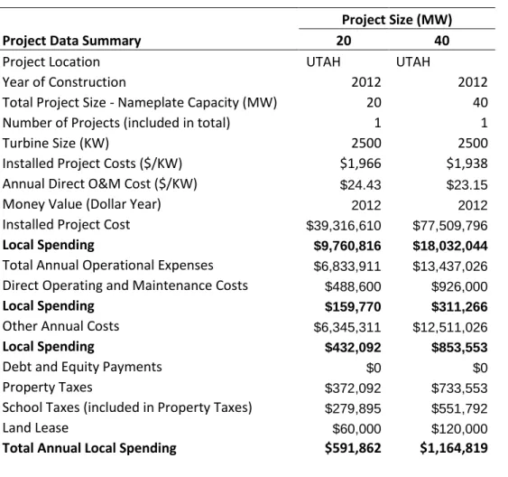
Table 1 (Project Data Summary) provides an overview of the economic impact results including local spending, property taxes (including tax revenues for Cache County School District), and lease payments for landowners. The average construction cost-per-kilowatt (kW) is expected to decrease as project size increases. The lines in bold type indicate the projected impacts that are related specifically to the state. For example, a modest 20-MW wind power installation could generate approximately $9.76 million in local spending during construction. During the first year of operations, about $592,000 in local spending would be incurred, which is the summation of about $160,000 in maintenance costs spent locally, $372,000 in county property taxes (of which $280,000 of those revenues is directed to the local school district), and $60,000 in lease payments made to local landowners. Details for other installation size scenarios are found in the three subsequent tables. Due to rounding, numbers in the tables may not sum exactly.
8 Table 1: Project Data Summary
Project Size (MW)
Project Data Summary 20 40
Project Location UTAH UTAH
Year of Construction 2012 2012
Total Project Size - Nameplate Capacity (MW) 20 40
Number of Projects (included in total) 1 1
Turbine Size (KW) 2500 2500
Installed Project Costs ($/KW) $1,966 $1,938
Annual Direct O&M Cost ($/KW) $24.43 $23.15
Money Value (Dollar Year) 2012 2012
Installed Project Cost $39,316,610 $77,509,796
Local Spending $9,760,816 $18,032,044
Total Annual Operational Expenses $6,833,911 $13,437,026
Direct Operating and Maintenance Costs $488,600 $926,000
Local Spending $159,770 $311,266
Other Annual Costs $6,345,311 $12,511,026
Local Spending $432,092 $853,553
Debt and Equity Payments $0 $0
Property Taxes $372,092 $733,553
School Taxes (included in Property Taxes) $279,895 $551,792
Land Lease $60,000 $120,000
Total Annual Local Spending $591,862 $1,164,819
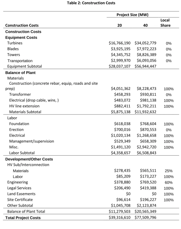
Table 2 provides a more detailed breakout of projected construction costs. The local share percentages in the right hand column were provided by Utah developers to derive the projected “local spending” to procure materials, services, and labor from Utah sources on the previous table (e.g., none of the wind turbines for a project in Cache County would be purchased in Utah given that no turbine manufacturers are operating in the state; however, 100 percent of the construction concrete rebar, etc. would be sourced locally given their availability). Using the 20-MW scenario as an example, the materials, labor, equipment, and other subtotals add up to about $39 million listed above as Total Project Costs (bottom of Table 2). Due to rounding, numbers in the tables may not sum exactly.
9
Table 2: Construction Costs
Project Size (MW) Construction Costs 20 40 Local Share Construction Costs Equipment Costs Turbines $16,766,190 $34,052,779 0% Blades $3,925,195 $7,972,223 0% Towers $4,345,752 $8,826,389 0% Transportation $2,999,970 $6,093,056 0% Equipment Subtotal $28,037,107 $56,944,447 Balance of Plant Materials
Construction (concrete rebar, equip, roads and site
prep) $4,051,362 $8,228,473 100%
Transformer $458,293 $930,811 0%
Electrical (drop cable, wire, ) $483,072 $981,138 100%
HV line extension $882,411 $1,792,211 100% Materials Subtotal $5,875,138 $11,932,632 Labor Foundation $618,038 $768,604 100% Erection $700,016 $870,553 0% Electrical $1,020,134 $1,268,658 100% Management/supervision $529,349 $658,309 100% Misc. $1,491,120 $2,942,720 100% Labor Subtotal $4,358,657 $6,508,843 Development/Other Costs HV Sub/Interconnection Materials $278,435 $565,511 25% Labor $85,209 $173,227 100% Engineering $378,880 $769,520 60% Legal Services $206,490 $419,388 100% Land Easements $0 $0 100% Site Certificate $96,614 $196,227 100% Other Subtotal $1,045,708 $2,123,874
Balance of Plant Total $11,279,503 $20,565,349
Total Project Costs $39,316,610 $77,509,796
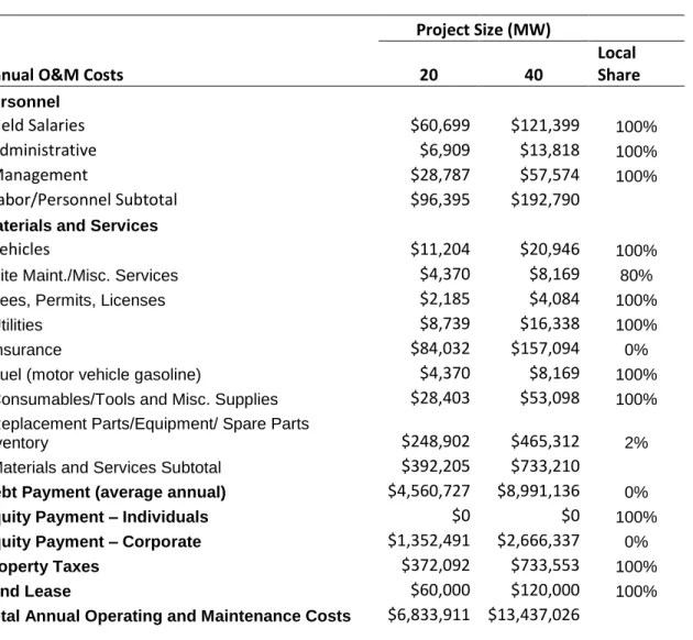
Table 3 (Operating and Maintenance Costs) provides details of project ongoing project expenditures, which form the basis of the estimates displayed in Table 1 in the row titled Total Annual Operational Expenses.
10
Table 3: Operating and Maintenance Costs
Project Size (MW)
Annual O&M Costs 20 40
Local Share Personnel Field Salaries $60,699 $121,399 100% Administrative $6,909 $13,818 100% Management $28,787 $57,574 100% Labor/Personnel Subtotal $96,395 $192,790
Materials and Services
Vehicles $11,204 $20,946 100%
Site Maint./Misc. Services $4,370 $8,169 80% Fees, Permits, Licenses $2,185 $4,084 100%
Utilities $8,739 $16,338 100%
Insurance $84,032 $157,094 0%
Fuel (motor vehicle gasoline) $4,370 $8,169 100% Consumables/Tools and Misc. Supplies $28,403 $53,098 100% Replacement Parts/Equipment/ Spare Parts
Inventory $248,902 $465,312 2%
Materials and Services Subtotal $392,205 $733,210
Debt Payment (average annual) $4,560,727 $8,991,136 0%
Equity Payment – Individuals $0 $0 100%
Equity Payment – Corporate $1,352,491 $2,666,337 0%
Property Taxes $372,092 $733,553 100%
Land Lease $60,000 $120,000 100%
Total Annual Operating and Maintenance Costs $6,833,911 $13,437,026
Table 4 utilizes the default values provided by the JEDI model in all fields except the local property tax rate, which for 2012 was 0.9464% (this figure includes the most significant tax assessments for Cache County and Cache County School District; individual city, mosquito abatement, library, and other
miscellaneous taxes are not included). These results use the local tax rate provided by the Cache County Assessor to more accurately predict total revenues. Specifically, the county tax levy rate multiplied by the assessed value of the wind project, which is predicted to be equal to total construction costs. Total construction cost for a 20-MW installation is about $39 million. Assessed at 100% taxable value, total projected annual county revenue for the first year is about $372,000, of which $280,000 would be directed to the local school district.
11
Table 4: Other Parameters
Project Size (MW)
Other Parameters 20 40 Local Share
Financial Parameters
Debt Financing
Percentage financed 80% 80% 0%
Years financed (term) 10 10
Interest rate 10% 10%
Equity Financing
Percentage equity 20% 20%
Individual Investors (percent of total equity) 0% 0% 100% Corporate Investors (percent of total equity) 100% 100% 0% Return on equity (annual interest rate) 16% 16%
Repayment term (years) 10 10
Tax Parameters
Local Property/Other Tax Rate (percent of taxable
value) 0.9464% 0.9464%
Assessed value (percent of construction cost) 100.0% 100.0% Taxable Value (percent of assessed value) 100.0% 100.0%
Taxable Value 39,316,610 77,509,796
Taxes per MW $11,120 $11,120
Local Taxes $372,092 $733,553 100%
School Taxes $279,895 $551,792
Land Lease Parameters
Land Lease Cost (per turbine) $7,500 $7,500
Land Lease (total cost) $60,000 $120,000
Lease Payment recipient (F = farmer/household, O
= Other) F F 100%
Payroll Parameters
Construction Labor (Average Wage Per Hour)
Employer Payroll Costs Foundation $13.82 $13.82 37.6% Erection $15.65 $15.65 37.6% Electrical $20.74 $20.74 37.6% Management/Supervision $28.19 $28.19 37.6%
O&M Labor (Average Wage Per Hour)
Employer Payroll Costs
Field Salaries (technicians, other) $18.86 $18.86 37.6%
Administrative $12.07 $12.07 37.6%
12
Table 5 (Estimated Number of Full-Time Equivalent Job Opportunities) includes results for the entire state of Utah, not limited to Cache County. This captures some of the broader state-level effects such as manufacturing and construction assets not necessarily available in Cache County. It does not include job opportunities that could result from state education and training programs to promote wind energy professional development and increase the state’s economic resource base. According to the table below, construction of a 20-MW installation would support 43 job opportunities from project development and on-site at a wind project, 40 of which are for construction. The total job
opportunities, including supply chain and induced effects, would total 153. During operating years, the wind park would produce two job opportunities on-site, with a total on-site, supply chain, and industry impact of six job opportunities. Due to rounding, numbers in the tables may not sum exactly.
Table 5: Estimated Number of Full-Time Job Opportunities
Project Size (MW)
Estimated FTE Jobs 20 40
During construction period
Project Development and Onsite Labor Impacts 43 56
Construction and Interconnection Labor 40 50
Construction Related Services 3 6
Local Revenue and Supply Chain Impacts 81 160
Induced Impacts 28 53
Total Impacts 153 269
During operating years (annual)
Onsite Labor Impacts 2 3
Local Revenue and Supply Chain Impacts 2 4
Induced Impacts 3 5
Total Impacts 6 12
Table 6 (Estimated Annual Wage and Salary Earnings) displays the potential earnings during the
construction period and the annual projected wages and salary earning during operation. For example, a 20-MW installation would produce total wage and salary earnings of approximately $7.3 million during construction (including $2.45 million from project development and on-site labor, $3.75 million from supply chain impacts, and $1.11 million from induced impacts), and annual wage and salary earnings of approximately $269,000 during operation. Due to rounding, numbers in the tables may not sum exactly.
13
Table 6: Estimated Annual Wage and Salary Earnings
Project Size (MW)
Economic Impacts – Earnings 20 40
During construction period
Project Development and Onsite Labor Impacts $2,454,235 $3,277,897
Construction and Interconnection Labor $2,243,812 $2,850,520 Construction Related Services $210,423 $427,378
Local Revenue and Supply Chain Impacts $3,747,507 $7,332,470
Induced Impacts $1,110,332 $2,052,488
Total Impacts $7,312,074 $12,662,855
During operating years (annual)
Onsite Labor Impacts $89,533 $179,066
Local Revenue and Supply Chain Impacts $80,311 $156,611
Induced Impacts $99,132 $195,193
Total Impacts $268,976 $530,921
Table 7 (Total Estimated Economic Output from Wind Park Development) displays the total projected increase in economic activity due to wind project installation and operation. Total impacts are broken down into total project development and on-site labor, supply chain impacts, and induced impacts during operation. To illustrate, a 20-MW installation is project to generate approximately $17.2 million in economic activity for the state of Utah during construction. During the first year in operations, total economic activity generated is projected to be about $1 million. Due to rounding, numbers in the tables may not sum exactly.
14
Table 7: Total Estimated Economic Output from Wind Park Development
Project Size (MW)
Economic Impacts – Output 20 40
During construction period
Project Development and Onsite Labor Impacts $2,686,628 $3,749,897
Construction and Interconnection Labor
Construction Related Services
Local Revenue and Supply Chain Impacts $10,998,897 $21,510,408
Induced Impacts $3,559,820 $6,580,451
Total Impacts $17,245,346 $31,840,756
During operating years (annual)
Onsite Labor Impacts $89,533 $179,066
Local Revenue and Supply Chain Impacts $650,795 $1,279,408
Induced Impacts $317,894 $625,943
Total Impacts $1,058,222 $2,084,417
Part III: Discussion and Conclusions Economic Benefits Summary
In summary, our economic projections indicate that development of wind power in Cache County poses significant economic opportunities for the state, benefiting the construction sector, schools, and landowners. For example, construction of a modest 20-MW wind project would generate about $17.2 million in economic impacts for the state (see Table 7); and once operational, in its first year, it would generate $372,000 in county tax revenues, of which $280,000 would go to Cache County schools, and $60,000 in lease payments to landowners (see Tables 1 and 3). Developing Utah’s wind resources, nonetheless, requires addressing some barriers and provision, including contradictory and/or changing municipal, state, and federal policies; project siting (e.g., zoning, accessing land leases, wildlife impact assessments, community acceptance); procuring power purchase agreements, turbines, and financing; and cultivating local community support (see Hartman, Stafford, and Reategui 2011; Stafford and Hartman 2012). While federal and state policies increasingly encourage wind power and other renewable energy development in Utah, approval of specific projects hinges on the support of county commissioners, city council members, mayors, local community leaders, and citizens. Understanding of the localized economic impacts created by the construction and operations of wind power plants can help decision makers evaluate the potential opportunities for their communities.
Additionally, to secure ongoing community support for wind power development, the potential economic impacts need to be “visible” in the community (Stafford and Hartman 2012). Property tax revenues from wind power, for example, can be substantive. They are often mixed, however, into county coffers where they become “invisible,” and local citizens may not recognize how the wind
15
turbines benefit their communities directly. Consequently, developers may negotiate with local officials to designate tax revenues to support high-profile community services and projects, such as sponsoring the local library or bookmobile, student scholarships, funding for parks and recreation programs, community youth athletics or other programs that often go unfunded in rural schools (Ratliff, Hartman and Stafford 2010; Stafford and Hartman 2012). When town and county residents connect visible improvement in their lives to local wind projects, enthusiasm for wind power can grow.
In Utah, because a substantial portion of property tax revenues generated from wind projects go directly to local school districts, wind developers and supporters may publicize a wind project’s potential direct tax revenue streams that will benefit rural schools and children. In 2003-4, the Utah Energy Offices sponsored an education outreach campaign with the message, “Wind Power Can Fund Schools”
(Hartman and Stafford 2010). It is important for wind developers and supporters to identify core values of a community such as school funding and frame wind power’s benefits to align with those values.
16 Appendix A. How the JEDI Model Works
The JEDI Model was developed by Marshall Goldberg (Goldberg, Sinclair, and Milligan 2004) to enable spreadsheet users with limited economic modeling experience to identify county-level, regional, and/or statewide economic impacts associated with constructing and operating wind power generation
facilities (i.e., “wind farms” or “wind parks”). JEDI’s “user add-in” feature allows researchers to conduct county-specific analyses using county IMPLAN (IMpact Analysis for PLANning) multipliers, while state-level multipliers are contained within the model as default values for all 50 states. IMPLAN was developed by the U.S. Forest Service to perform regional economic analyses. Presently, IMPLAN
software and data are managed and updated by the Minnesota IMPLAN Group, Inc., using data collected at federal, state, and local levels. The analysis in this report used JEDI model version W1.10.03, which uses 2010 multiplier data from the Minnesota IMPLAN Group.
JEDI is an “input-output” model, an analytical tool developed to trace supply linkages in the economy (Goldberg, Sinclair, and Milligan 2004). JEDI attempts to measure spending patterns and location-specific economic structures that reflect expenditures supporting varying levels of employment, income, and output. For example, JEDI reveals how purchases of wind project materials, such as wind turbines or other materials, not only potentially benefit local turbine manufacturers, but also the local fabrication metals industry, concrete rebar, drop cable, wire, etc., given that such industries may exist in the county or state, and expenditures will be made locally.
Input-output analysis is a method of evaluating and summing three economic impacts: (1) project development and on-site labor, (2) turbine and supply chain impacts, and (3) induced effects. These are defined below with respect to wind park construction and operation:
Project Development and On-site Labor effects: During the construction of wind parks, this refers to the on-site jobs of contractors and crews hired and project development. During operations, this refers to on-site labor only.
Turbine, Supply Chain, and Local Revenue effects: During the construction of wind projects, this category refers to the impact of expenditures made for turbines and the supply chain (e.g., steel manufacturers that supply towers, hardware stores that provide building supplies for construction crews, or electric-utility suppliers that procure goods, such as high-voltage transmission lines [Costanti 2004]). During operations, this category refers to local revenues generated by the project (e.g., land lease payments) and expenditures in the supply chain (e.g., spare parts, fuel for on-site vehicles, materials and services, etc.).
Induced effects: Induced effects are changes in earnings that are induced by the spending of businesses and persons related to the project development, on-site labor, turbine, supply chain, and local revenues by the wind project. Induced effects would include spending on food, clothing, retail services, public transportation, gasoline, vehicles, property and income taxes, medical services, and the like.
17
The sum of these three effects yields the total economic effects that result from expenditures on the construction and operation of a wind park (Goldberg, Sinclair, and Milligan 2004). In determining economic effects, the model considers 14 aggregated industries that are impacted by the construction and operation or a wind park (agriculture, construction, electrical equipment, fabricated metals, finance/insurance/real estate, government, machinery, mining, other manufacturing, other services, professional service, retail trade, transportation/communication/public utilities, and wholesale trade). Estimates are made using state- and county-level multipliers and personal expenditure patterns; these multipliers for employment, wage and salary income and output (economic activity), and personal expenditure come from IMPLAN (IMPLAN 2006).
18 Appendix B. Applying the JEDI Model
The model is programmed in Microsoft Excel, and it requires four sets of inputs: (1) Project Descriptive Data; (2) Project Cost Data; (3) Annual Wind Plant Operating and Maintenance Costs; and (4) Other Parameters.
The Project Descriptive Data consists of eight parameters: Project location (county/state location)
Year of construction
Project size (nameplate capacity) Turbine size (kilowatt or kW size) Number of turbines
Project construction cost (dollars per kilowatt capacity or $/kW) Annual operation and maintenance cost ($/kW)
Money value – current dollar year.
The Project Cost Data consists of 16 parameters organized into three categories: Construction costs
Equipment costs
Other miscellaneous costs.
Annual Wind Plant Operating and Maintenance Costs consist of 11 parameters organized into two categories:
Personnel
Materials and services.
The Other Parameters section is the last section of inputs, consisting of 17 inputs organized into five categories:
19 Equity financing/repayment
Tax parameters Land lease parameters Payroll parameters.
Regarding the expenditure pattern and the local share of expenditures for a particular county, region, or state, assumptions play a significant role in determining the economic impact of a wind project. The JEDI Model provides two options: (1) default values or (2) new local and product-specific values entered by the analyst.
The default values represent a “reasonable expenditure pattern for constructing and operating a wind power plant in the United States and the share of expenditures spent locally… based on a review of numerous wind resource studies” (Goldberg, Sinclair, and Milligan 2004, p. 3). Not every wind project, however, will follow this exact “default” pattern for expenditure. Consequently, analysts are
encouraged to incorporate project-specific data and the likely share of spending in a given county, region, or state to reflect localized economic impacts. In our analysis, we’ve consulted with a local wind developer to determine reasonable local spending levels for specific costs associated with this wind project.
20 Appendix C. JEDI Model Outputs
The JEDI Model generates the following outputs for a given set of inputs: Jobs: Refers to the annual full-time equivalent employment.
Output: The economic activity or “project value” in the state, region, or county economy. Earnings: Refers to annual wage and/or salary compensations (including other
employer-provided supplements, including retirement) paid to workers involved with on-site labor, supply chain, or induced effects.
Local Spending: Refers to the actual annual dollars spent on goods and services in the area being analyzed (state, regional, or county economy where the wind park is being built).
Annual Lease Payments: Provides an annual total of lease/easement payments to landowners. Property Taxes: Represents the annual property taxes that the project will generate, exclusive
21 Appendix D. JEDI Model Limitations
As with other economic projection tools, JEDI has several assumptions and limitations (Costanti 2004). For example, JEDI is not intended to be a precise forecasting tool. Rather, it provides a reasonable profile of how investment in a wind plant may affect a given economy. Additionally, JEDI offers a gross analysis rather than a net analysis; that is, the model does not account for the net impacts associated with alternate spending of project funds or replacement of existing electricity generation facilities that may exist within a given local economy (e.g., electricity generation by wind replacing electricity
generated by an existing gas-fired generation plant). JEDI also assumes that adequate revenue exists to cover all debt and/or equity payments and annual operations and maintenance costs associated with a given project. Consequently, while JEDI can provide analysts with the reasonable benefits associated with a given project, wind developers, utility managers, and government officials need to ensure that a given project is an acceptable investment.
22 Appendix E. Some Insight into IMPLAN
The JEDI model was developed for the National Renewable Energy Lab by Marshall Goldberg (Goldberg, 2003) to allow individuals with minimal modeling experience to easily simulate and predict regional economic impacts associated with installation of wind projects. To achieve its results, the JEDI model uses the inputs described in the preceding text, determines the portion of the spending which will impact the region of interest, and then uses the IMPLAN multipliers from that region to determine how much impact that portion of the spending will have via the labor, supply chain, and induced impacts discussed previously in the introduction to the JEDI model.
IMPLAN (Impact Analysis for Planning) was developed by Scott Lindall and Doug Olson at the University of Minnesota in close conjunction with the U.S. Forest Service’s Land Management Planning Unit. In 1993, a technology transfer agreement with the University of Minnesota allowed the formation of the Minnesota IMPLAN Group, Inc. (MIG, Inc.) which currently manages all IMPLAN products.
The following excerpt from the introduction of “The IMPLAN Input-Output System” provides a brief description of how the IMPLAN multipliers are derived:
Input-output accounting describes commodity flows from producers to intermediate and final consumers. The total industry purchases of commodities, services, employment compensation, value added, and imports are equal to the value of the commodities produced.
Purchases for final use (final demand) drive the model. Industries produce goods and services for final demand and purchase goods and services from other producers. These other producers, in turn, purchase goods and services. This buying of goods and services (indirect purchases) continues until leakages from the region (imports and value added) stop the cycle.
These indirect and induced effects (the effects of household spending) can be mathematically derived. The derivation is called the Leontief inverse. The resulting sets of multipliers describe the change of output for each and every regional industry caused by a one dollar change in final demand for any given industry (Lindall and Olson, 2008).
In this analysis the IMPLAN multipliers for the state of Utah were used to calculate the labor, supply chain, and induced impacts of the change in final demand in wind energy and associated industries, based on the cost projections provided in the preceding report.
23 References
Barry, J., Hurlbut, D., Simon, R., Moore, Jl. & Blackett, R. (2009). Utah Renewable Energy Zones Task Force Phase I Report: Renewable Energy Zone Resource Identification. Miscellaneous Publication 09-1, Utah Geological Survey, Utah Department of Natural Resources.
http://www.energy.utah.gov/renewable_energy/docs/2009/Jan/mp-09-1low.pdf (last accessed May 2013).
Cartledge, J. (2010). “Construction Gets Underway at 102 MW Wind Project in Utah,”
AggregateResearch.com, April 29. https://aggregateresearch.com/articles/19091/Construction-gets-underway-at-102MW-wind-project-in-Utah.aspx. (Last accessed May 2013).
Costanti, M. (2004). Quantifying the Economic Development Impacts of Wind Power in Six Rural Montana Counties Using NREL’s JEDI Model. Report NREL/SR-500-36414. Golden, CO: National Renewable Energy Laboratory.
Del Franco, M. (2013). “Wind Developers Receive Clarity on PTC Requirements,” North American Windpower, May, pp. 1, 27.
Del Franco, M. (2012a). “Pressure Applied in States To Widen RPS Allowances,” North American Windpower, May, pp. 1, 24.
Del Franco, M. (2012b). “Windbearings,” North American Windpower, May, p. 4.
First Wind Press Release. (2009). “Milford Wind Corridor Project is Completed; Largest Wind Facility in Utah and One of the Largest in the West. November 10.
http://www.firstwind.com/sites/default/files/Milford_Ribbon-cutting_Press%20Release_FINAL_111009.pdf. (Last accessed May 2013).
First Wind Press Release. (2011). “First Wind Begins Commercial Operations of Milford Wind II Wind Project. May 9. http://eon.businesswire.com/news/eon/20110509006800/en/scppa/beaver-county/wind-energy. (Last accessed May 2013).
Goldberg, M. (2003). “Wind Impact Model.” Goldberg and Associates, 2003.
Goldberg, M.; Sinclair, K.; and Milligan, M. (2004). Job and Economic Development Impact (JEDI) Model: A User-Friendly Tool to Calculate Economic Impacts from Wind Projects. Prepared for the 2004 Global WINDPOWER Conference, March 2004. NREL/CP-500-28010. Golden, CO: National Renewable Energy Laboratory.
Gramlich, R. (2013). “U.S. Wind Industry is Back on Track,” enerG, March/April, p. 32.
Hartman, C.L. and Stafford E.R. (2010). “Sell the Wind,” Stanford Social Innovation Review, Winter, 25-6. Hartman, C.L.; Stafford, E.R.; and Reategui, S. (2011). “Harvesting Utah’s Urban Winds,” Solutions
24
Hollenhorst, J. (2012). “Proposed Monticello Wind Farm Stirs the Air with Controversy,” Deseret News, October 24. http://www.deseretnews.com/article/865564463/Proposed-Monticello-wind-farm-stirs-the-air-with-controversy.html?pg=all. (Last accessed May 2013).
IMPLAN (2006). IMPLAN. Minnesota IMPLAN Group, Inc. Stillwater, MN. Available at:
www.implan.com.
Lindall, S.A.; Olson, D.C. (2008). “The IMPLAN Input-Output System.” IMPLAN 2.0 io System Description; Stillwater, Minnesota; 28 February 2008,
ftp://ftp-fc.sc.egov.usda.gov/Economics/NatImpact/implan_io_system_description.pdf.
Martin, C. (2013a). “U.S. States Turn Against Renewable Energy as Gas Plunges,” Bloomberg, April 23.
http://www.bloomberg.com/news/2013-04-23/u-s-states-turn-against-renewable-energy-as-gas-plunges.html (Last accessed May 2013).
Martin, C. (2013b). “North Carolina Rejects Cuts to Renewable Energy Mandates,” Bloomberg, April 24.
http://www.bloomberg.com/news/2013-04-24/north-carolina-rejects-cuts-to-renewable-energy-mandates.html (Last accessed May 2013).
Mohl, B. (2013). “Gordon: Cape Wind Launches This Year,” CommonWealth, February 26.
http://www.commonwealthmagazine.org/News-and-Features/Online-exclusives/2013/Winter/021-Gordon-Cape-Wind-launches-this-year.aspx. (Last accessed May 2013).
Ratliff, D.J.; Hartman, C.L.; and Stafford, E.R. (2010). An Analysis of State-Level Economic Impacts from the Development of Wind Power Plants in San Juan County, Utah. March 2010. DOE/GO-102010-3005. Golden, CO: U.S. Department of Energy, Energy Efficiency and Renewable Energy.
Reategui, S.; Stafford, E.R.; Hartman, C.L.; Huntsman, J.M. (January 2009). Generating Economic Development from a Wind Power Project in Spanish Fork Canyon, Utah: A Case Study and Analysis of State-Level Economic Impacts. DOE/GO-102009-2760. Golden, CO: U.S. Department of Energy, Energy Efficiency and Renewable Energy.
http://www.windpoweringamerica.gov/pdfs/economic_development/2009/ut_spanish_fork.pdf. (Last accessed May 2013).
Reuters. (2013). “U.S. Wind power Grows At Record Levels – AWEA,” May 13.
http://www.reuters.com/article/2013/03/13/utilities-wind-awea-idUSL1N0C549C20130313. (Last accessed May 2013).
Stafford, E.R. and Hartman, C.L. (2012). “Resolving Community Concerns over Local Wind Development in Utah,” Sustainability: The Journal of Record, 5 (February), 38-43.
U.S. Department of Energy. (2008), 20% Wind Energy by 2030, Energy Efficiency and Renewable Energy, DOE/GO-102008-2567. http://www.20percentwind.org/20percent_wind_energy_report_revOct08.pdf. (Last accessed May 2013).
25
Zuhlke, K. (2012). “More Utilities Choosing Wind Power.” Windpower Update, 2012 Pre-Show Issue, p. 16-17.