How To Solve The Pde Problem On A Mesh With A Freefem++ (Freefemplest) On A Computer Or A Computer (For Freefems)

(1)

FreeFem++

Manual

version 1.42(Under construction)

http://www.freefem.org

http://www.ann.jussieu.fr/˜hecht/freefem++.htm

F. Hecht

1

, O. Pironneau

2

,

Universit´

e Pierre et Marie Curie,

Laboratoire Jacques-Louis Lions,

175 rue du Chevaleret ,PARIS XIII

K. Ohtsuka

3

,

Hiroshima Kokusai Gakuin University, Hiroshima, Japan

September 6, 2004

1_{mailto:[email protected]} 2_{mailto:[email protected]} 3_{mailto:[email protected]}

(2)

(3)

6.6.1 Cavity.edp . . . 63 6.6.2 StokesUzawa.edp . . . 66 6.6.3 NSUzawaCahouetChabart.edp . . . 67 6.7 Readmesh.edp . . . 68 6.8 Domain decomposition . . . 69 6.8.1 Schwarz-overlap.edp . . . 69 6.8.2 Schwarz-no-overlap.edp . . . 71 6.8.3 Schwarz-gc.edp . . . 72 6.9 Beam.edp . . . 74 6.10 Fluidstruct.edp . . . 75 6.11 Region.edp . . . 78 6.12 FreeBoundary.edp . . . 80 6.13 nolinear-elas.edp . . . 83

7 Parallel version experimental 89 7.1 Schwarz in parallel . . . 89

8 The Graphic User Interface (FFedit) 91 8.1 Unix version . . . 91

8.1.1 Installation of Tcl and Tk . . . 91

8.1.2 Description . . . 92

8.1.3 Cygwin version . . . 94

8.1.4 Installation of Cygwin . . . 95

8.1.5 Compilation and Installation of FreeFem++ under Cygwin . . . 95

8.1.6 Compilation and Installation of tcl8.4.0 and tk8.4.0 under Cygwin . . 96

8.1.7 Use . . . 99

9 Mesh Files 101 9.1 File mesh data structure . . . 101

9.2 bb File type for Store Solutions . . . 102

9.3 BB File Type for Store Solutions . . . 102

(5)

CONTENTS 5

9.5 List of AM FMT, AMDBA Meshes . . . 103

10 Add new finite element 107 10.1 Some notation . . . 107

10.2 Which class of add . . . 108

10.3 How to add . . . 111

11 Grammar 113 11.1 Keywords . . . 113

11.2 The bison grammar . . . 113

11.3 The Types of the languages, and cast . . . 117

11.4 All the operators . . . 122

(6)

(7)

Chapter 1 Introduction

A partial differential equation is a relation between a function of several variables and its (partial) derivatives. Many problems in physics, engineering, mathematics and even banking are modeled by one or several partial differential equations.

Freefem is a software to solve these equations numerically. As its name says, it is a free software (see copyright for full detail) based on the Finite Element Method. This software runs on all unix OS (with g++ 2.95.2 or better and X11R6) , on Window95, 98, 2000, NT, XP, on MacOS 9 and X.

Many phenomena involve several different fields. Fluid-structure interactions, Lorenz forces in liquid aluminium and ocean-atmosphere problems are three such systems. These require approximations of different degrees, possibly on different meshes. Some algorithms such as Schwarz’ domain decomposition method also require data interpolation on different meshes within one program. freefem++ can handle these difficulties, i.e. arbitrary finite element spaces on arbitrary unstructured and adapted meshes.

The characteristics of freefem++ are:

• A large variety of finites elements : linear and quadratic Lagrangian elements, discon-tinuous P1 and Raviart-Thomas elements, elements of a non-scalar type, mini-element, ...

• Automatic interpolation of data on different meshes to an over mesh.

• Linear problems description thanks to a formal variational form, with access to the vectors and the matrix if needed.

• Includes tools to define discontinuous Galerkin formulations (please refer to the follow-ing keywords: “jump”, “average”, “intalledges”)

• Analytic description of boundaries. When two boundaries intersect, the user must specify the intersection points.

• Automatic mesh generator, based on the Delaunay-Voronoi algorithm. Inner points density is proportional to the density of points on the boundary [5].

(8)

• Metric-based anisotropic mesh adaptation. The metric can be computed automatically from the Hessien of a solution [6].

• Solvers : LU, Cholesky, Crout, CG, GMRES, UMFPACK linear solver, eigenvalue and eigenvector computation.

• Online graphics, C++-like syntax.

• Many examples: Navier-Stokes, elasticity, Fluid structure, Schwarz’s domain decom-position method, Eigen value problem, residual error indicator, ...

• Parallel version using mpi

1.1 History

The project has evolved from MacFem, PCfem, written in Pascal. The first C version was

freefem 3.4; it offered mesh adaptation on a single mesh. A thorough rewriting in C++ led to freefem+ 1.2.10, which also included interpolation over multiple meshes (func-tions defined on one mesh can be used on any other mesh). Implementing the interpolation from one unstructured mesh to another was not easy because it had to be fast and non-diffusive; for each point, one had to find the containing triangle. This is one of the basic problems of computational geometry (see Preparata & Shamos[10] for example). Doing it in a minimum number of operations was a challenge. Our implementation was O(nlogn) and based on a quadtree.

We are now introducingfreefem++ , an entirely new program written in C++ and based onbison for a more adaptable freefem language.

The freefem language allows for a quick specification of any partial differential system of equations. The language syntax of freefem++ is the result of a new design which makes use of the STL [15], templates andbisonfor its implementation. The outcome is a versatile software in which any new finite element can be included in a few hours; but a recompilation is then necessary. The library of finite elements available in freefem++ will therefore grow with the version number. So far we have linear and quadratic Lagrangian elements, discontinuous P1 and Raviart-Thomas elements.

1.2 The language

Basically freefem++ is a compiler. The language it defines is typed, polymorphic and reentrant with macro generation (see 6.13). Every variable must be typed and declared in a statement; each statement separated from the next by a semicolon ‘;’.

Here is a simple example solving the Dirichlet problem inside the unit circle. We have chosen

xy as the right hand side for the Laplace operator, a second degree finite element method on triangles, and a mesh with 50 points on the boundary. The linear system is solved by a Gauss LU factorisation.

(9)

1.3. INSTALLATION 9

border a(t=0,2*pi){x=cos(t); y=sin(t);label=5;};

mesh Th = buildmesh (a(50));

fespace Vh(Th,P2); Vh u,v;

func f= x*y;

problem laplace(u,v,solver=LU) =

int2d(Th)(dx(u)*dx(v) + dy(u)*dy(v)) // bilinear part

- int2d(Th)( f*v) // right hand side

+ on(5,u=0) ; // Dirichlet boundary condition

real cpu=clock();

laplace; // SOLVE THE PDE

plot(u);

cout << " CPU = " << clock()-cpu << endl;

Reserved words are shown in blue. pi, x, y, label, solver are reserved variables. It is allowed (although not advisable) to redefine these variables, so they will not be high-lighted again in the following example programs.

This example shows some of the characteristics of freefem++ :

• Boundaries are described analytically (by opposition to CSG). In the case where two boundaries intersect, the user must specify the intersection points in case two bound-aries intersect. The domain will be on the left side of the oriented boundary.

• Automatic mesh generation, based on the Delaunay-Voronoi algorithm. Inner points are generated with a density proportional to the density of points on the boundary (hence a refined mesh is obtained by increasing the number of boundary points). • Preprogrammed library of arbitrary degree elements.

• Every variable is typed. For instance fis a function, specified by the keyword func. • Online graphics (see the documentation below for zoom, postscript and other

com-mands).

• C++-like syntax.

1.3 Installation

There are binary packages available for Microsoft Windows and Apple Mac OS. For all other platforms,freefem++ must be compiled and installed from the source archive. This

archive is available fromhttp://www.ann.jussieu.fr/˜hecht/ftp/freefem/freefem+ +.tgz. To extract files from the compressed archive freefem++.tgz into a directory

called freefem++-X.XX (where X.XX is the version number) enter the following commands in a shell window :

tar zxvf freefem++.tgz cd freefem++-X.XX

(10)

To compile and install freefem++ , just follow the INSTALL and README files. The following programs are produced, depending on the system you are running (Linux, Windows, MacOS) :

1. FreeFem++, standard version, with a graphical interface based on X11, Win32 or MacOS

2. FreeFem++-nw, postscript output only (batch version, no windows) 3. FreeFem++-mpi, parallel version, postscript output only

4. FreeFem++-glx, graphics using OpenGL and X11

5. /Applications/FreeFem++.app, Drag and Drop CoCoa MacOs Application 6. FreeFem++-CoCoa, MacOS Shell script for MacOS OpenGL version (MacOS 10.2

or better) (note: it uses /Applications/FreeFem++.app)

As an installation test, go into the directoryexamples++-tutorialand runfreefem++

on the example script LaplaceP1.edp with the command :

(11)

Chapter 2 Syntax

2.1 Data Types

Every variable must be declared together with its type. The language allows the manip-ulation of basic types : integers (int), reals (real), strings (string), arrays (example:

real[int]), bidimensional (2D) finite element meshes (mesh), 2D finite element spaces (fespace), finite element functions (fespace variable), functions (func), arrays of finite element functions (fespace variable[basictype]), linear and bilinear operators, sparse matrices, vectors, etc. For instance :

int i,n=20; // i, n∈Z

real pi=4*atan(1.); // pi∈R(redef ine)

real[int] xx(n),yy(n); // two array of size n

for (i=0;i<=20;i++) // which can be used in statements such as this

{ xx[i]= cos(i*pi/10); yy[i]= sin(i*pi/10); }

whereint,real,complexcorrespond to the C typeslong,double,complex<double>.

The scope of a variable is the current block (delimited by “{. . .}”) as in C++ , except the

fespace variable. The variables which are local to a block are destroyed at the end of the block.

Type declarations are compulsory in freefem++ . This is necessary to prevent many potential programming errors related to type mismatch. A variable name is just an al-phanumeric string. The underscore character is not allowed because it will be used as an operator in the future.

2.1.1 Another Example

real r= 0.01;

mesh Th=square(10,10); // unit square mesh

fespace Vh(Th,P1); // P1 lagrange finite element space

Vh u = x+ exp(y);

(12)

func f = z * x + r * log(y);

plot(u,wait=1);

{ // new block

real r= 2; // not the same r

fespace Vh(Th,P1); // error because Vh is a global name

}

// here r==0.01

Note 1 Notice the use of wait to monitor the time a graph stays on screen (i.e. the time freefem stops before going to the next instruction).

2.2 List of major types

bool a C++ true, false value;

int long integer; string aC++ string; real double;

complex complex<double>;

ofstream ofstream to output to a file ifstream ifstream to input from a file real[int] array of reals (integer index);

real[int,int] matrix of reals (2 integers indices); real[string] array of reals (string index);

string[string] array of string (string index); mesh[int] array of meshes (integer index);

func define a function (on one line, without arguments) func f=cos(x)+sin(y);. Please note that the function type is given by the type of the expression.

mesh defines a mesh. e.g. mesh Th=buildmesh(circle(10));

fespace to define a new type of finite element space. e.g. fespace Vh(Th,P1);. At present, the available finite elements are :

P0 constant discontinuous finite element

P1 linear piecewise continuous finite element

P2 P2 piecewise continuous finite element, where P2 is the set of polynoms of R2 of degree two,

RT0 the Raviart-Thomas finite element,

P1nc non-conforming P1 finite element,

P1dc linear piecewise discontinuous finite element

(13)

2.3. GLOBALS 13 P1b linear piecewise continuous finite element + bubble

To definepas a function belonging to fespaceVh: Vh p;. T odefineaas an array of 10 functions from Vh: Vh a[10];

problem defines a pde problem without solving it. solve defines a pde problem and solves it.

varf defines a full variational form. matrix defines a sparse matrix.

Constant values for the above type can be : true is a constant of type bool,

false is a constant of type bool, 123 is an integer,

123. is of type real,

123.e10 is a constant of type real and value 123 1010. Please note that the syntax of a real number is the same as inC++ or fortran.

"abcd" is a constant of type string. There are two escape characters allowed in string constants : \nto insert a newline and\"to insert a".

2.3 Globals

The following names are related to the underlying finite element abstractions :

x the x coordinate of the current point (real value)

y the y coordinate of the current point (real value)

z the z coordinate of the current point (real value), (reserved for future use).

label the boundary label number of the current point if it is on a boundary, otherwise 0 (integer value).

region a function returning the region number of the current point (x,y,z). Integer value.

P current point (_R3 value. P.x, P.y, P.z)

N normal vector at the current point (_R3 _value, _N.x_, _N.y_, _N.z_{) .}

lenEdge length of the current edge

hTriangle size of the current triangle

(14)

nuEdge integer index of the current edge in the triangle

nTonEdge integer: number of triangle contening the current edge (1 or 2).

area area of the current triangle

cout consoleostream

cin console istream

true bool value

false boolvalue

pi realapproximation of π endl the end of line string

Here is how to show all types, operators and functions from inside afreefem++ program :

dumptable(cout);

To run a system command stored in a string (not implemented on Carbon MacOs) :

exec("shell command");

2.4 Arithmetic

The available operators are the usual C operators:

+ - * / \% ˜ ˆ | || & && ! == != < > <= >= = += -= *= /= << >> ++ -- ,

with the same meaning as in C++ except for

• ˆ which is the power operator (with right precedence as in math or in maple),

• | & ! are the three boolean operators ‘or’ , ‘and’ , ‘not’

• ’ .* ./ are array operators (as in matlab or scilab), where

– ’is the unary right transposition of an array or a matrix

– .*is the term by term multiply operator.

– ./is the term by term divide operator. some compound operators:

– ˆ-1 means solving a linear system (example: b = Aˆ-1 x)

– ’ *is a transposition followed by a matrix product, i.e. the dot product (example

(15)

2.4. ARITHMETIC 15 As inC++ , there are automatic casts from a type to another. So in some sense we have

bool⊂int⊂real ⊂complex

and if any of these four types is copied into a string, it will be converted into a human-readable value. Example: basics real x=3.14,y; int i,j; complex c; cout << " x = " << x << "\n"; x = 1;y=2; x=y; i=0;j=1; cout << 1 + 3 << " " << 1/3 << "\n"; cout << 10 ˆ10 << "\n"; cout << 10 ˆ-10 << "\n"; cout << -10ˆ-2+5 << "== 4.99 \n"; cout << 10ˆ-2+5 << "== 5.01 \n"; cout << "--- complex ---- \n" ; cout << 10-10i << " \n"; cout << " -1ˆ(1/3) = " << (-1+0i)ˆ(1./3.) << " \n"; cout << " 8ˆ(1/3)= " << (8)ˆ(1./3.) << " \n"; cout << " sqrt(-1) = " << sqrt(-1+0i) << " \n";

cout << " ++i =" << ++i ;

cout << " i=" << i << "\n";

cout << " i++ = "<< i++ << "\n";

cout << " i = " << i << "\n"; // ---- string concatenation ---string str,str1; str="abc+"; str1="+abcddddd+"; str=str + str1; // string concatenation str = str + 2 ; cout << "str= " << str << "== abc++abcddddd+2;\n"; R3 P; P.x=1; x=P.x; cout <<"P.x = "<< P.x << endl;

output displayed on the console:

x = 3.14 4 0 1e+10 1e-10 4.99== 4.99 5.01== 5.01 -- complex ----(10,-10)

(16)

-1ˆ(1/3) = (0.5,0.866025) 8ˆ(1/3)= 2 sqrt(-1) = (6.12323e-17,1) ++i =1 i=1 i++ = 1 i = 2 str= abc++abcddddd+2== abc++abcddddd+2; P.x = 1

The usual mathematical functions are implemented:

sqrt, pow, exp, log, sin, cos, atan, cosh, sinh, tanh, min, max, etc... And usualC++ functions are implemented: exit, assert

2.5 Array

There are 2 kinds of arrays: arrays with integer indices and arrays with string indices. In the first case, the size of this array must be known at execution time, and the implemen-tation is done with the KN<> class so all the vector operations of KN<> are implemented. It

is also possible to build an array of FE functions with the same syntax.

The second case is just a map of the STL1[15] so no vector operation is allowed, except for the selection of an item.

The transpose operator is ’ (as in MathLab or SciLab), so the way to compute the dot product of two arrays a,b isreal ab= a’*b.

int i;

real [int] tab(10), tab1(10); // 2 arrays of 10 reals

real [int] tab2; // bug! missing array size

tab = 1; // set all array elements to 1

tab[1]=2;

cout << tab[1] << " " << tab[9] << " size of tab = "

<< tab.n << " " << tab.min << " " << tab.max << " " << endl; tab1=tab;

tab=tab+tab1; tab=2*tab+tab1*5; tab1=2*tab-tab1*5; tab+=tab;

cout << " dot product " << tab’*tab << endl; // ttab tab

cout << tab << endl;

cout << tab[1] << " " << tab[9] << endl;

real[string] map; // a dynamic array

for (i=0;i<10;i=i+1) { tab[i] = i*i; cout << i << " " << tab[i] << "\n"; }; map["1"]=2.0;

map[2]=3.0; // 2 is automatically cast to the string "2" 1_{Standard template Library, now part of standard}_C++

(17)

2.6. LOOPS 17

cout << " map[\"1\"] = " << map["1"] << "; "<< endl;

cout << " map[2] = " << map[2] << "; "<< endl;

string[string] tt; // a array of string

2.6 Loops

for and while loops are implemented, with the same semantics as in C++ , including keywords break and continue.

int i; for (i=0;i<10;i=i+1) cout << i << "\n"; real eps=1; while (eps>1e-5) { eps = eps/2; if( i++ <100) break;

cout << eps << endl;}

2.7 Input/Output

The syntax of input/output statements is similar toC++ syntax. It usescout,cin,endl,

<<,>>.

To write to (resp. read from) a file, declare a new variableofstream ofile("filename");

orofstream ofile("filename",append);(resp. ifstream ifile("filename");

) and use ofile (resp. ifile) as cout (resp. cin). The word append in ofstream ofile("filename",append); means opening a file in append mode.

Note 2 The file is closed at the end of the enclosing block,

int i;

cout << " std-out" << endl;

cout << " enter i= ? ";

cin >> i ; {

ofstream f("toto.txt"); f << i << "coucou’\n";

}; // file f closed here because variable f is deleted

{

ifstream f("toto.txt"); f >> i;

} {

ofstream f("toto.txt",append); // appending data to file "toto.txt"

f << i << "coucou’\n";

}; // file f closed here because variable f is deleted

(18)

(19)

Chapter 3 Mesh Generation

The following keywords are discussed in this section:

square, border, buildmesh, movemesh , adaptmesh, readmesh, trunc, triangulate, splitmesh, emptymesh

All the examples in this section come from the filesmesh.edpandtablefunction.edp.

3.1 Square

For easy and simple testing we have included a constructor for rectangles. All other shapes should be handled with borderand buildmesh. The following

real x0=1.2,x1=1.8;

real y0=0,y1=1;

int n=5,m=20;

mesh Th=square(n,m,[x0+(x1-x0)*x,y0+(y1-y0)*y]);

mesh th=square(4,5);

plot(Th,th,ps="twosquare.eps");

constructs an×m grid in the rectangle [1.2,1.8]×[0,1] and a 4×5 grid in the unit square [0,1]2_.

Note 3 Boundary labels are numbered 1,2,3,4 for bottom, right, top, left side (before the mapping [x0 + (x1−x0)∗x, y0 + (y1−y0)∗y] (the mapping can be non linear).

3.2 Border

A domain is defined as being on the left (resp right) of its parameterized boundary (when looking towards increasing values of the parameter) if the sign of the expression that returns the number of vertices on the boundary is positive (resp negative).

note: the boundary label must be non-zero if you you want to specify a boundary condition on this border

For instance the domain delimited by the unit circle, with a small circular hole inside would be described as:

real pi=4*atan(1);

(20)

Figure 3.1: The 2 square meshes

border a(t=0,2*pi){ x=cos(t); y=sin(t);label=1;}

border b(t=0,2*pi){ x=0.3+0.3*cos(t); y=0.3*sin(t);label=2;}

plot(a(50)+b(+30)) ; // to see a plot of the border mesh

mesh Thwithouthole= buildmesh(a(50)+b(+30));

mesh Thwithhole = buildmesh(a(50)+b(-30));

plot(Thwithouthole,wait=1,ps="Thwithouthole.eps"); // figure 3.2

plot(Thwithhole,wait=1,ps="Thwithhole.eps"); // figure 3.3

Note 4 The use of ps="fileName" generates a postscript file identical to the plot shown on screen.

Figure 3.2: mesh without hole Figure 3.3: mesh with hole

(21)

3.3. MOVEMESH 21

3.3 Movemesh

As the two last statements in the example below show, mesh motion is possible. Some-times the moved mesh is invalid because some triangle becomes reversed (with a negative area). This is why we check the minimum triangle area in the transformed mesh with

checkmovemesh before any real transformation.

real Pi=atan(1)*4; verbosity=4; border a(t=0,1){x=t;y=0;label=1;}; border b(t=0,0.5){x=1;y=t;label=1;}; border c(t=0,0.5){x=1-t;y=0.5;label=1;}; border d(t=0.5,1){x=0.5;y=t;label=1;}; border e(t=0.5,1){x=1-t;y=1;label=1;}; border f(t=0,1){x=0;y=1-t;label=1;}; func uu= sin(y*Pi)/10;

func vv= cos(x*Pi)/10;

mesh Th = buildmesh ( a(6) + b(4) + c(4) +d(4) + e(4) + f(6));

plot(Th,wait=1,fill=1,ps="Lshape.eps"); // see figure ??

real coef=1;

real minT0= checkmovemesh(Th,[x,y]); // the min triangle area

while(1) // find a correct move mesh

{

real minT=checkmovemesh(Th,[x+coef*uu,y+coef*vv]);// the min triangle area

if (minT > minT0/5) break ; // if big enough

coef=/1.5; }

Th=movemesh(Th,[x+coef*uu,y+coef*vv]);

plot(Th,wait=1,fill=1,ps="movemesh.eps"); // see figure 3.5

(22)

Note 5 Consider a function u defined on a mesh Th. A statement likeTh=movemesh(Th... does not change u and so the old mesh still exists. It will be destroyed when no function use it. A statement like u=u redefines u on the new mesh Th with interpolation and therefore destroys the old Th if u was the only function using it.

Now, an example of moving mesh, with lagrangian function u defined on the moving mesh.

// simple movemesh example

mesh Th=square(10,10);

fespace Vh(Th,P1);

real t=0;

//

---// the problem is how to build data without interpolation // so the data u is moving with the mesh as you can see in the plot

//

---Vh u=y;

for (int i=0;i<4;i++) {

t=i*0.1; Vh f= x*t;

real minarea=checkmovemesh(Th,[x,y+f]);

if (minarea >0 ) // movemesh will be ok

Th=movemesh(Th,[x,y+f]);

cout << " Min area " << minarea << endl; real[int] tmp(u[].u);

tmp=u[]; // save the value

u=0; // to change the FEspace and mesh associated with u

u[]=tmp; // set the value of u without any mesh update

plot(Th,u,wait=1); };

// In this program, since u is only defined on the last mesh, all the // previous meshes are deleted from memory.

//

---3.4

Reading and writing a mesh

Freefem can read and write files. A mesh file can be read back into freefem++ but the names of the borders are lost. So these borders have to be referenced by the number which corresponds to their order of appearance in the program, unless this number is forced by the keyword ”label”.

border floor(t=0,1){ x=t; y=0; label=1;}; // the unit square

border right(t=0,1){ x=1; y=t; label=5;};

border ceiling(t=1,0){ x=t; y=1; label=5;};

border left(t=1,0){ x=0; y=t; label=5;};

int n=10;

mesh th= buildmesh(floor(n)+right(n)+ceiling(n)+left(n));

savemesh(th,"toto.am_fmt"); // "formatted Marrocco" format

savemesh(th,"toto.Th"); // "bamg"-type mesh

(23)

3.5. TRIANGULATE 23

savemesh(th,"toto.nopo"); // modulef format see [7]

mesh th2 = readmesh("toto.msh"); // read the mesh

There are many mesh file formats available for communication with other tools such as emc2, modulef... The suffix gives the chosen type. More details can be found in the article by F. Hecht ”bamg : a bidimentional anisotropic mesh generator” available from the freefem web page.

3.5 Triangulate

freefem++ is able to build a triangulation from a set of points. This triangulation is a Delaunay mesh of the convex hull of the set of points. It can be useful to build a table function.

The coordinates of the points and the value of the table function are defined in a separate file which looks like :

0.51387 0.175741 0.636237 0.308652 0.534534 0.746765 0.947628 0.171736 0.899823 0.702231 0.226431 0.800819 0.494773 0.12472 0.580623 0.0838988 0.389647 0.456045

The third column of each line is left untouched by the triangulate command. But you can use this third value to define a table function with rows of the form: x y f(x,y).

mesh Thxy=triangulate("xyf"); // build the Delaunay mesh of the convex hull // points are defined by the first 2 columns of file xyf

plot(Thxy,ps="Thxyf.ps"); // (see figure ??)

fespace Vhxy(Thxy,P1); // create a P1 interpolation

Vhxy fxy; // the function

// reading the third row to define the function

{ ifstream file("xyf");

real xx,yy;

for(int i=0;i<fxy.n;i++)

file >> xx >>yy >> fxy[][i]; // to read third row only. xx and yy are just skipped

}

plot(fxu,ps="xyf.ps"); // plot the function (see figure ??)

3.6 Adaptmesh

Mesh adaptation is a very powerful tool which should be used whenever possible. freefem++

uses a variable metric/Delaunay automatic meshing algorithm. It takes one or more func-tions as input (see in the following example) and builds a mesh adapted to the second derivative of the given function.

(24)

verbosity=2; mesh Th=square(10,10,[10*x,5*y]); fespace Vh(Th,P1); Vh u,v,zero; u=0; u=0; zero=0; func f= 1; func g= 0; int i=0;

real error=0.1, coef= 0.1ˆ(1./5.);

problem Problem1(u,v,solver=CG,init=i,eps=-1.0e-6) = //

int2d(Th)( dx(u)*dx(v) + dy(u)*dy(v)) + int2d(Th) ( v*f )

+ on(1,2,3,4,u=g) ;

real cpu=clock(); for (i=0;i< 10;i++) {

real d = clock(); Problem1;

plot(u,zero,wait=1);

Th=adaptmesh(Th,u,inquire=1,err=error);

cout << " CPU = " << clock()-d << endl; error = error * coef;

} ;

cout << " CPU = " << clock()-cpu << endl;

This method is described in detail in [6]. It has a number of default parameters which can be modified :

hmin= Minimum edge size. (val is a double precision value. Its default is related to the size of the domain to be meshed and the precision of the mesh generator).

hmax= Maximum edge size. (val is a double precision value. It defaults to the diameter of the domain to be meshed)

err= P1 interpolation error level (0.01 is the default).

errg= Relative geometrical error. By default this error is 0.01, and in any case it must be lower than 1/√2. Meshes created with this option may have some edges smaller than the -hmin argument due to geometrical constraints.

nbvx= Maximum number of vertices generated by the mesh generator (9000 is the default).

nbsmooth= number of iterations of the smoothing procedure (5 is the default).

nbjacoby= number of iterations in a smoothing procedure during the metric construction, 0 means no smoothing (6 is the default).

(25)

3.6. ADAPTMESH 25

ratio= ratio for a prescribed smoothing on the metric. If the value is 0 or less than 1.1 no smoothing is done on the metric (1.8 is the default).

If ratio > 1.1, the speed of mesh size variations is bounded by log(ratio). Note: As ratio gets closer to 1, the number of generated vertices increases. This may be useful to control the thickness of refined regions near shocks or boundary layers .

omega= relaxation parameter for the smoothing procedure (1.0 is the default).

iso= If true, forces the metric to be isotropic (false is the default).

abserror= If false, the metric is evaluated using the criterium of equi-repartion of relative error (false is the default). In this case the metric is defined by

M= 1 err coef2 |H| max(CutOff,|η|) p (3.1)

otherwise, the metric is evaluated using the criterium of equi-distribution of errors. In this case the metric is defined by

M= 1 err coef2 |H sup(η)−inf(η) p . (3.2)

cutoff= lower limit for the relative error evaluation (1.0e-6 is the default).

verbosity= informational messages level (can be chosen between 0 and ∞). Also changes the value of the global variable verbosity (obsolete).

inquire= To inquire graphicaly about the mesh (false is the default).

splitpbedge= If true, splits all internal edges in half with two boundary vertices (true is the default).

maxsubdiv= Changes the metric such that the maximum subdivision of a background edge is bound by val (always limited by 10, and 10 is also the default).

rescaling= if true, the function with respect to which the mesh is adapted is rescaled to be between 0 and 1 (true is the default).

keepbackvertices= if true, tries to keep as many vertices from the original mesh as possible (true is the default).

isMetric= if true, the metric is defined explicitly (false is the default). If the 3 functions

m11, m12, m22 are given, they directly define a symmetric matrix field whose Hessian

is computed to define a metric. If only one function is given, then it represents the isotropic mesh size at every point.

power= exponent power of the Hessian used to compute the metric (1 is the default).

(26)

splitin2= boolean value. If true, splits all triangles of the final mesh into 4 sub-triangles.

metric= an array of 3 real arrays to set or get metric data information. The size of these three arrays must be the number of vertices. So if m11,m12,m22are three P1 finite el-ements related to the mesh to adapt, you can write: metric=[m11[],m12[],m22[]]

(see file convect-apt.edp for a full example)

nomeshgeneration= If true, no adapted mesh is generated (useful to compute only a metric).

periodic= use: builds an adapted periodic mesh, you can writeperiodic=[[4,y],[2,y],[1,x],[3,x]];

to build a biperiodic mesh of a square. (see periodic finite element spaces 4, and see

sphere.edpfor a full example)

3.7 Trunc

A small operator to create a truncated mesh from a mesh with respect to a boolean function. The two named parameter

label= sets the label number of new boundary item (one by default)

split= sets the level n of triangle splitting. each triangle is splitted in n×n ( one by default).

To create the mesh Th3 where alls triangles of a meshThare splitted in 3×3 , just write:

mesh Th3 = trunc(Th,1,split=3);

The truncmesh.edp example construct all ”trunc” mesh to the support of the basic function of the space Vh (cf. abs(u)>0), split all the triangles in 5×5, and put a label number to 2 on new boundary.

fespace Vh(Th,P1); Vh u;

int i,n=u.n; u=0;

for (i=0;i<n;i++) // all degre of freedom

{

u[][i]=1; // the basic function i

plot(u,wait=1);

mesh Sh1=trunc(Th,abs(u)>1.e-10,split=5,label=2);

plot(Th,Sh1,wait=1,ps="trunc"+i+".eps"); // plot the mesh of

// the function’s support

u[][i]=0; // reset

(27)

3.8. SPLITMESH 27

Figure 3.6: mesh of support the function P1 number 0, splitted in 5×5

Figure 3.7: mesh of support the function P1 number 6, splitted in 5×5

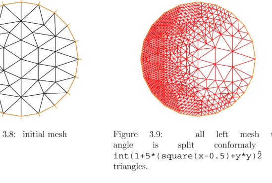
3.8 splitmesh

A other way to split mesh triangle:

{ // new stuff 2004 splitmesh (version 1.37)

assert(version>=1.37);

plot(Th,wait=1,ps="nosplitmesh.eps"); // see figure 3.8

mesh Th=buildmesh(a(20));

plot(Th,wait=1);

Th=splitmesh(Th,1+5*(square(x-0.5)+y*y));

plot(Th,wait=1,ps="splitmesh.eps"); // see figure 3.9

}

3.9 build empty mesh

The idea is when you want to defined Finite Element space on boundary you can use a mesh with no internal points (call empty mesh). It is can by useful we you have a Lagrange multiplier definied on the border.

So the function emptymesh remove all the internal point of a mesh expect if the point is on internal boundary.

{ // new stuff 2004 emptymesh (version 1.40)

// -- useful to build Multiplicator space // build a mesh without internal point

// with the same boundary

//

---assert(version>=1.40);

mesh Th=buildmesh(a(20)); Th=emptymesh(Th);

(28)

Figure 3.8: initial mesh Figure 3.9: all left mesh tri-angle is split conformaly in

int(1+5*(square(x-0.5)+y*y)ˆ2

triangles.

}

or it is also possible to build a empty mesh of peusdo subregion withemptymesh(Th,ssd)

with the set of edges of the mesh Th a edge e is in this set if the two adjacent triangles

e = t1 ∩t2 and ssd[T1] 6= ssd[T2] where ssd defined the peusdo region numbering of triangle. It is an userint[int] array of size the number of triangles.

{ // new stuff 2004 emptymesh (version 1.40) // -- useful to build Multiplicator space // build a mesh without internal point

// of peusdo sub domain

//

---assert(version>=1.40); mesh Th=square(10,10); int[int] ssd(Th.nt);

for(int i=0;i<ssd.n;i++) // build the peusdo region numbering

{ int iq=i/2; // because 2 traingle per quad

int ix=iq%10; //

int iy=iq/10; //

ssd[i]= 1 + (ix>=5) + (iy>=5)*2; }

Th=emptymesh(Th,ssd); // build emtpy with

// all edge e=T1∩T2 and ssd[T1]6=ssd[T2]

plot(Th,wait=1,ps="emptymesh-2.eps"); // see figure 3.11

savemesh(Th,"emptymesh-2.msh"); }

3.10 Get Mesh numbering

(29)

3.11. MESHING EXAMPLES 29

Figure 3.10: The empty mesh with bound-ary

Figure 3.11: An empty mesh defined from a peusdo region numbering of triangle

// get data of the mesh

int nbtriangles=Th.nt;

for (int i=0;i<nbtriangles;i++)

for (int j=0; j <3; j++)

cout << i << " " << j << " Th[i][j] = "

<< Th[i][j] << " x = "<< Th[i][j].x << " , y= "<< Th[i][j].y << ", label=" << Th[i][j].label << endl;

}

the output is:

0 0 Th[i][j] = 0 x = 0 , y= 0, label=4 0 1 Th[i][j] = 1 x = 0.5 , y= 0, label=1 0 2 Th[i][j] = 4 x = 0.5 , y= 0.5, label=0 1 0 Th[i][j] = 0 x = 0 , y= 0, label=4 1 1 Th[i][j] = 4 x = 0.5 , y= 0.5, label=0 1 2 Th[i][j] = 3 x = 0 , y= 0.5, label=4 ... 5 2 Th[i][j] = 6 x = 0 , y= 1, label=4 6 0 Th[i][j] = 4 x = 0.5 , y= 0.5, label=0 6 1 Th[i][j] = 5 x = 1 , y= 0.5, label=2 6 2 Th[i][j] = 8 x = 1 , y= 1, label=3 7 0 Th[i][j] = 4 x = 0.5 , y= 0.5, label=0 7 1 Th[i][j] = 8 x = 1 , y= 1, label=3 7 2 Th[i][j] = 7 x = 0.5 , y= 1, label=3

3.11 Meshing examples

Example: 1: The mesh for a corner singularity The domain is an L-shape:

(30)

border b(t=0,0.5){x=1;y=t;label=1;};

border c(t=0,0.5){x=1-t;y=0.5;label=1;};

border d(t=0.5,1){x=0.5;y=t;label=1;};

border e(t=0.5,1){x=1-t;y=1;label=1;};

border f(t=0,1){x=0;y=1-t;label=1;};

mesh rh = buildmesh (a(6) + b(4) + c(4) +d(4) + e(4) + f(6));

Example: 2: Meshes for domain decompositions To test the domain decomposition algo-rithms described below we will need 2 overlapping meshes of a single domain.

border a(t=0,1){x=t;y=0;};

border a1(t=1,2){x=t;y=0;};

border b(t=0,1){x=2;y=t;};

border c(t=2,0){x=t ;y=1;};

border d(t=1,0){x = 0; y = t;};

border e(t=0, pi/2){ x= cos(t); y = sin(t);};

border e1(t=pi/2, 2*pi){ x= cos(t); y = sin(t);}; n=4;

mesh sh = buildmesh(a(5*n)+a1(5*n)+b(5*n)+c(10*n)+d(5*n)); mesh SH = buildmesh ( e(5*n) + e1(25*n) );

plot(sh,SH);

Example: 3: Meshes for fluid-structure interactions Two rectangles touching by a side.

border a(t=0,1){x=t;y=0;}; border b(t=0,1){x=1;y=t;}; border c(t=1,0){x=t ;y=1;}; border d(t=1,0){x = 0; y=t;}; border c1(t=0,1){x=t ;y=1;}; border e(t=0,0.2){x=1;y=1+t;}; border f(t=1,0){x=t ;y=1.2;}; border g(t=0.2,0){x=0;y=1+t;}; int n=1;

mesh th = buildmesh(a(10*n)+b(10*n)+c(10*n)+d(10*n));

mesh TH = buildmesh ( c1(10*n) + e(5*n) + f(10*n) + g(5*n) );

(31)

Chapter 4 Finite Elements

To use a finite element, one needs to define a finite element space with the keywordfespace

(short of finite element space) like

fespace IDspace(IDmesh,<IDFE>) ;

or withk pair of periodic boundary condition

fespace IDspace(IDmesh,<IDFE>,

periodic=[[la1,sa1],[lb 1,sb1], ...

[lak,sa k],[lbk,sb k]]);

where IDspaceis the name of the space for exampleVh,IDmeshis the name of the associated

mesh and <IDFE> is a identifier of finite element type, where a pair of periodic boundary

condition is defined by [lai,sai],[lbi,sbi]. The int expressions lai and lbi are defined

the 2 labels of the piece of the boundary to be equivalence, and the real expressions sai

and sbi a give two common abcissa on the two boundary curve, and two points are identify

if the two abcissa are equal.

As of today, the known types of finite element are:

P0 piecewise constante discontinuous finite element

P0h ={v ∈L2(Ω) ; ∀K ∈ Th ∃αK ∈R: v|K =αK} (4.1)

P1 piecewise linear continuous finite element

P1h ={v ∈H1(Ω) ; ∀K ∈ Th v|K ∈P1} (4.2)

P1dc piecewise linear discontinuous finite element

P1dch ={v ∈L2(Ω) ; ∀K ∈ Th v|K ∈P1} (4.3)

P1b piecewise linear continuous finite element plus bubble

P1bh =

v ∈H1(Ω) ; ∀K ∈ Th v|K ∈P1⊕Span{λK0 λK1 λK2 } (4.4)

where λK_i , i= 0,1,2 are the 3 barycentric coordinate functions of the triangle K

(32)

P2 piecewise P2 continuous finite element,

P2h ={v ∈H1(Ω) ; ∀K ∈ Th v|K ∈P2} (4.5)

where P2 is the set of polynomials of R2 of degrees at most 2.

P2dc piecewise P2 discontinuous finite element,

P2dch ={v ∈L2(Ω) ; ∀K ∈ Th v|K ∈P2} (4.6)

RT0 Raviart-Thomas finite element

RT0h ={v∈H(div)/∀K ∈ Th v|K(x, y) = αK βK +γK| x y } (4.7)

where H(div) is the set of function of L2(Ω) with divergence in L2(Ω), and where

αK, βK, γK are real numbers.

P1nc piecewise linear element continuous at the middle of edge only. To define the finite element spaces

Xh ={v ∈H1(]0,1[2) ; ∀K ∈ Th v|K ∈P1} Xph ={v ∈Xh ; v(|0. ) = v(|1. ), v(| . 0) = v(|1. )} Mh ={v ∈H1(]0,1[2) ; ∀K ∈ Th v|K ∈P2} Rh ={v∈H1(]0,1[2)2 ; ∀K ∈ Th v|K(x, y) = αK βK +γK| x y }

where T is a mesh 10×10 of the unit square ]0,1[2, the corresponding freefem++ definitions are:

mesh Th=square(10,10); // border label: 1 down, 2 left, 3 up, 4 right

fespace Xh(Th,P1); // scalar FE

fespace Xph(Th,P1,periodic=[[2,y],[4,y],[1,x],[3,x]]); // bi-periodic FE

fespace Mh(Th,P2); // scalar FE

fespace Rh(Th,RT0); // vectorial FE

soXh,Mh,Rhare finite element spaces (called FE spaces ). Now to use functionsuh, vh ∈Xh

and ph, qh ∈Mh and Uh, Vh ∈Rh one can define the FE function like this Xh uh,vh;

Xph uph,vph; Mh ph,qh;

Rh [Uxh,Uyh],[Vxh,Vyh];

Xh[int] Uh(10); // array of 10 function in Xh

Rh[int] [Wxh,Wyh](10); // array of 10 functions in Rh.

The functions Uh, Vh have two components so we have

Uh = U xh_{U yh} and V_h = V xh_{V yh} .

(33)

33 Like in the previous version, freefem+, the finite element functions (type FE functions) are both functions from _R2 _to

RN with N = 1 for scalar function and arrays of real.

To interpolate a function, one writes

uh = xˆ2 + yˆ2; // ok uh is scalar FE function

[Uxh,Uyh] = [sin(x),cos(y)]; // ok vectorial FE function

Uxh = x; // error: impossible to set only 1 component

// of a vector FE function.

vh = Uxh; // ok

Th=square(5,5);

vh=vh; // re-interpolates vh on the new mesh square(5,5);

vh([x-1/2,y])= xˆ2 + yˆ2; // interpole vh = ((x−1/2)2₊_Y2₎ To get the value at a point x= 1, y = 2 of the FE function uh, or [Uxh,Uyh],one writes

real value;

value = uh(2,4); // get value= uh(2,4)

value = Uxh(2,4); // get value= Uxh(2,4)

// or

---x=1;y=2;

value = uh; // get value= uh(1,2)

value = Uxh; // get value= Uxh(1,2)

value = Uyh; // get value= Uyh(1,2).

To get the value of the array associated to the FE function uh, one writes

real value = uh[][0] ; // get the value of degree of freedom 0

real maxdf = uh[].max; // maximum value of degree of freedom

int size = uh.n; // the number of degree of freedom

real[int] array(uh.n)= uh[]; // copy the array of the function uh

Warning for no scalar finite element function[Uxh,Uyh]the two arrayUxh[]and Uyh[]

are the same array, because the degre of freedom can touch more than one componant. The other way to set a FE function is to solve a ‘problem’ (see below).

Note 6 It is possible to change a mesh to do a convergence test for example, but see what happens in this trivial example. In fact a FE function is three pointers, one pointer to the values, second a pointer to the definition offespace, third a pointer to thefespace. This fespace can be rebuild if the associated mesh have changed when the FE function is set with operator = or when a problem is solved.

mesh Th=square(2,2);

fespace Xh(Th,P1); Xh uh,vh;

vh= xˆ2+yˆ2; // vh

Th = square(5,5); // change the mesh

// Xh is unchange

uh = xˆ2+yˆ2; // compute on the new Xh

// and now uh use the 5x5 mesh // but the fespace of vh is alway the 2x2 mesh

plot(vh,ps="onoldmesh.eps"); // figure 4.1

vh = vh; // do a interpolation of vh (old) of 5x5 mesh // to get the new vh on 10x10 mesh.

(34)

Figure 4.1: vh Iso on mesh 2×2 Figure 4.2: vh Iso on mesh 5×5

4.1 Problem and solve

For freefem++ a problem must be given in variational form, so a bilinear form, a linear form, and possibly a boundary condition form must be input. For example consider the Dirichlet problem:

−∆v = 1 in Ω =]0,1[2, v = 0 on Γ =∂Ω. The problem can be solved by the finite element method, namely:

Find uh ∈ V0h the space of continuous piecewise linear functions on a triangulation of Ω

which are zero on the boundary ∂Ω such that

Z Ω ∇uh · ∇wh = Z Ω wh ∀wh ∈V0h

The freefem++ version of the same is

fespace Vh(Th,P1); // P1 FE space

Vh uh,vh; // unknown and test function.

func f=1; // right hand side function

func g=0; // boundary condition function

solve laplace(uh,vh) = // definion of the problem and solve

int2d(Th)( dx(uh)*dx(vh) + dy(uh)*dy(vh) ) // bilinear form

+ int2d(Th)( -f*vh ) // linear form

+ on(1,2,3,4,uh=g) ; // a lock boundary condition form

f=x+y;

laplace; // solve again the problem with this new f

plot(uh,ps="Laplace.eps",value=true); // to see the result (figure 4.3)

Note 7 Using the keywork problem in place of solve would define the problem only and not solve it.

(35)

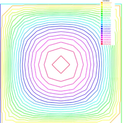
4.1. PROBLEM AND SOLVE 35 IsoValue 0.00182747 0.0054824 0.00913734 0.0127923 0.0164472 0.0201021 0.0237571 0.027412 0.0310669 0.0347219 0.0383768 0.0420317 0.0456867 0.0493416 0.0529965 0.0566515 0.0603064 0.0639613 0.0676163 0.0712712

Figure 4.3: Isovalues of the solution

A laplacian in mixed finite formulation .

mesh Th=square(10,10); fespace Vh(Th,RT0); fespace Ph(Th,P0); Vh [u1,u2],[v1,v2]; Ph p,q; problem laplaceMixte([u1,u2,p],[v1,v2,q],solver=LU,eps=1.0e-30) = //

int2d(Th)( p*q*1e-10+ u1*v1 + u2*v2 + p*(dx(v1)+dy(v2)) + (dx(u1)+dy(u2))*q ) + int2d(Th) ( q)

+ int1d(Th)( (v1*N.x +v2*N.y)/-2); // int on gamma

laplaceMixte; // the problem is now solved

plot([u1,u2],coef=0.1,wait=1,ps="lapRTuv.eps",value=true); // figure 4.4

plot(p,fill=1,wait=1,ps="laRTp.eps",value=true); // figure 4.5

Vec Value 0 0.0168845 0.0337689 0.0506534 0.0675378 0.0844223 0.101307 0.118191 0.135076 0.15196 0.168845 0.185729 0.202613 0.219498 0.236382 0.253267 0.270151 0.287036 0.30392 0.320805 Figure 4.4: Flux (u1, u2) IsoValue -0.502006 -0.496373 -0.492618 -0.488862 -0.485107 -0.481352 -0.477597 -0.473842 -0.470086 -0.466331 -0.462576 -0.458821 -0.455066 -0.45131 -0.447555 -0.4438 -0.440045 -0.43629 -0.432534 -0.423146 Figure 4.5: Isovalue of p

(36)

Note 8 To make programs more readable we stop now using blue color on dx,dy.

An other formulation of the Laplace equation with Discontinuous Galerkine formulation with

P2 discontinuous can be write (see LapDC.epd and [17])

// file: LapDG2.edp

// solve −∆u=f on Ω and u=g on Γ macro dn(u) (N.x*dx(u)+N.y*dy(u) ) // def the normal derivative

mesh Th = square(10,10); // unite square

fespace Vh(Th,P2dc); // Discontinous P2 finite element // if pena = 0 => Vh must be P2 otherwise we need some penalisation

real pena=0; // a paramater to add penalisation

varf Ans(u,v)=

int2d(Th)(dx(u)*dx(v)+dy(u)*dy(v) )

+ intalledges(Th)( // loop on all edge of all triangle // the edge are see nTonEdge times so we / nTonEdge // remark: nTonEdge =1 on border edge and =2 on internal // we are in a triange th normal is the exterior normal // def: jump = external - internal value; on border exter value =0

// average = (external + internal value)/2, on border just internal value

( jump(v)*average(dn(u)) - jump(u)*average(dn(v)) + pena*jump(u)*jump(v) ) / nTonEdge ) ; func f=1; func g=0; Vh u,v; Xh uu,vv; problem A(u,v,solver=UMFPACK) // = Ans - int2d(Th)(f*v) - int1d(Th)(g*dn(v) + pena*g*v) ; problem A1(uu,vv,solver=CG) // =

int2d(Th)(dx(uu)*dx(vv)+dy(uu)*dy(vv)) - int2d(Th)(f*vv) + on(1,2,3,4,uu=g);

A; // solve DG

where

• nTonEdgeis the number on triangle which see the current edge, withnTonEdge==2

on internal edge andnTonEdge==1 on boundary edge,

• jump give the jump in the direction of the external normal: external minus internal value on internal edges, and minus the internal value

• average is the half of the external plus internal value on internal edges and the internal value on boundary edges.

(37)

4.2. PARAMETER DESCRIPTION FOR SOLVE ANDPROBLEM 37

4.2 Parameter Description for

solve

and

problem

The parameters are FE function, the numbern of qfo is even (n = 2∗k), thek first function parameters are unknown, and thek last are test functions.

Note 9 If the functions are a part of vectoriel FE then you must give all the functions of the vectorial FE in the same order (see laplaceMixte problem for example).

Bug: 1 The mixing of fespace with differents periodic boundary condition is not imple-mented. So all the finite element space use for test or unknow functions in a problem, must have the same type of periodic boundary condition or no periodic boundary condition. No clean message is given and the result is impredictible, Sorry.

The named parameters are:

solver= LU, CG,Crout,Cholesky,GMRES,UMFPACK ...

The default solver isLU. The storage mode of the matrix of the underlying linear system depends on the type of solver chosen; for LU the matrix is sky-line non symmetric, for Crout the matrix is sky-line symmetric, for Cholesky the matrix is sky-line symmetric positive definite, for CG the matrix is sparse symmetric positive, and for

GMRES orUMFPACK the matrix is just sparse.

eps= a real expression. ε sets the stopping test for the iterative methods likeCG. Note that if ε is negative then the stopping test is:

||Ax−b||<|ε| if it is positive then the stopping test is

||Ax−b||< |ε|

||Ax0−b||

init= boolean expression, if it is false or 0 the matrix is reconstructed. Note that if the mesh changes the matrix is reconstructed too.

precon= name of a function (for example P) to set the precondioner. The prototype for the function P must be

func real[int] P(real[int] & xx) ;

tgv= Huge value (1030), to lock boundary conditions

4.3 Problem definition

Below v is the unknown function and wis the test function. After the ”=” sign, one may find sums of:

(38)

• the bilinear form term: -) int2d(Th)( K*v*w) = X T∈Th Z T K v w -) int2d(Th,1)( K*v*w) = X T∈Th,T⊂Ω1 Z T K v w -) int1d(Th,2,5)( K*v*w) = X T∈Th Z (∂T∪Γ)∩(Γ2∪Γ5) K v w -) intalledges(Th)( K*v*w) = X T∈Th Z ∂T K v w -) intalledges(Th,1)( K*v*w) = X T∈Th,T⊂Ω1 Z ∂T K v w

-) a sparse matrix of type matrix

• the linear form term:

-) int1d(Th)( K*w) = X T∈Th Z T K w -) int1d(Th,2,5)( K*w) = X T∈Th Z (∂T∪Γ)∩(Γ2∪Γ5) K w -) intalledges(Th)( f*w) = X T∈Th Z ∂T f w

-) a vector of type real[int]

• The boundary condition form term :

– An ”on” form (for Dirichlet ) : on(1, u = g )

– a linear form on Γ (for Neumann ) -int1d(Th))( f*w) or -int1d(Th,3))( f*w)

– a bilinear form on Γ or Γ2(for Robin ) int1d(Th))( K*v*w) or int1d(Th,2))( K*v*w).

If needed, the different kind of terms in the sum can appear more than once.

Remark: the integral mesh and the mesh associated to test function or unkwon function can be different in the case of linear form.

Note 10 N.x and N.y are the normal’s components.

Important: it is not possible to write in the same integral the linear part and the bilinear part such as in int1d(Th)( K*v*w - f*w) .

(39)

4.4. INTEGRALS 39

4.4 Integrals

There are three kinds of integrals:

• surface integral defined with the keyword int2d

• integrals on curves int1d.

• integrals on the three edges of all triangles intalledges, remark the edges are see two times generaly (the variable nTonEdge give this number).

the syntaxe is :

keywork(domain_parameters)( function )

where the (domain parameters) given the definition of the domain of integration and the kind of quadrature formulae.

The (domain parameters) can be : • (Th) ???

• (Th,1)???

• (Th,1,qforder=2) ???

• (Th,1,qft= qf3pT, qfe= qf2pE) ??? where whereTh is a mesh.

Integrals can be used to define the variational form, or to compute integrals proper. It is possible to choose the order of the integration formula by adding a parameterqforder=to define the order of the Gauss formula, or directly the name of the formula withqft=name

in 2d integrals and qfe=name in 1d integrals. The quadrature formulae on triangles are:

name (qft=) on order qforder= exact number of quadrature points

qf1pT triangle 2 1 1

qf1pTlump triangle 4 3

qf2pT4P1 triangle 2 9

The quadrature formulae on edges are:

name (qfe=) on order qforder= exact number of quadrature points

qf1pE segment 2 1 1

qf2pE segment 3 2 2

(40)

4.5 Variational Form, Sparse Matrix, Right Hand Side Vector

It is possible to define variational forms:

fespace Xh(Th,P2),Mh(Th,P1); Xh u1,u2,v1,v2;

Mh p,q,ppp;

varf bx(u1,q) = int2d(Th)( (dx(u1)*q));

bx(u1, q) =

Z

Ωh

∂u1

∂xq

varf by(u1,q) = int2d(Th)( (dy(u1)*q));

by(u1, q) =

Z

Ωh

∂u1

∂y q

varf a(u1,u2)= int2d(Th)( dx(u1)*dx(u2) + dy(u1)*dy(u2) ) + on(1,2,4,u1=0) + on(3,u1=1) ;

a(u1, v2) =

Z

Ωh

∇u1.∇u2; u1 = 1∗g on Γ3, u1 = 0 on Γ1∪Γ2∪Γ4

where f is defined later.

Later variational forms can be used to construct right hand side vectors, matrices associated to them, or to define a new problem;

Xh bc1; bc1[] = a(0,Xh); // right hand side for boundary condition

Xh b;

matrix A= a(Xh,Xh,solver=CG); // the Laplace matrix

matrix Bx= bx(Xh,Mh); // Bx= (Bxij) and Bxij =bx(bxj, b m j ) // where bx_j is a basis of Xh, and bm_j is a basis of Mh.

matrix By= by(Xh,Mh); // By= (Byij) and Byij =by(bxj, b m j )

Note 11 The line of the matrix corresponding to test function on the bilinear form.

Note 12 The vector bc1[] contains the contribution of the boundary condition u1 = 1.

Here we have three matrices A, Bx, By, and we can solve the problem: find u1 ∈Xh such that

a(v1, u1) = by(v1, f),∀v1 ∈X0h,

u1 =g, on Γ1,and u1 = 0 on Γ1∪Γ2∪Γ4

with the following line (where f =x, and g =sin(x))

Mh f=x; Xh g=sin(x);

(41)

4.6. EIGEN VALUE AND EIGEN VECTOR 41

b[] = Bx’*f[]; //

b[] += bc1[] .*bcx[]; // u1= g on Γ3 boundary see following remark

u1[] = Aˆ-1*b[]; // solve the linear system

Note 13 The boundary condition is implemented by penalization and the vector bc1[] contains the contribution of the boundary condition u1 = 1 , so to change the boundary condition, we have just to multiply the vector bc1[] by the value f of the new boundary condition term by term with the operator .*. The StokesUzawa.edp 6.6.2 gives a real example of using all this features.

We add automatic expression optimization by default, if this optimization trap you can remove the use of this optimization by writing for example :

varf a(u1,u2)= int2d(Th,optimize=false)( dx(u1)*dx(u2) + dy(u1)*dy(u2) ) + on(1,2,4,u1=0) + on(3,u1=1) ;

4.6 Eigen value and eigen vector

This section depend of your FreeFem++ compilation process (see README arpack), to compile this tools. This tools is available in FreeFem++if the word ”eigenvalue” appear in line ”Load:”, like:

-- FreeFem++ v1.28 (date Thu Dec 26 10:56:34 CET 2002) file : LapEigenValue.edp

Load: lg_fem lg_mesh eigenvalue

This tools is base on the arpack++ 1 the object-oriented version of ARPACK eigenvalue package [?, arpack]

The function EigenValue compute the generalized eigenvalue ofAu =λBu where sigma =σ

is the shift of the method. The matrix OP is defined withA−σB. The return value is the number of converged eigenvalue (can be greater than the number of eigen value nev=)

int k=EigenValue(OP,B,nev= , sigma= );

where the matrix OP =A−σB with a solver and boundary condition, and the matrix B.

sym= the problem is symmetric (all the eigen value are real)

nev= the number desired eigenvalues (nev) close to the shift.

value= the array to store the real part of the eigenvalues

ivalue= the array to store the imag. part of the eigenvalues

vector= the array to store the eigenvectors. For real nonsymmetric problems, complex eigenvectors are given as two consecutive vectors, so if eigenvalue k and k + 1 are complex conjugate eigenvalues, thekth vector will contain the real part and thek+1th vector the imaginary part of the corresponding complex conjugate eigenvectors.

(42)

tol= the relative accuracy to which eigenvalues are to be determined;

sigma= the shift value;

maxit= the maximum number of iterations allowed;

ncv= the number of Arnoldi vectors generated at each iteration of ARPACK.

In the first example, we compute the eigenvalue and the eigenvector of the Dirichlet problem on square Ω =]0, π[2_.

The problem is find: λ, and ∇uλ in R×H01(Ω)

Z

Ω

∇uλ∇v =λintΩuv ∀v ∈H01(Ω)

The exact eigenvalues are λn,m = (n2+m2),(n, m) ∈ N∗2 with the associated eigenvectors

are um,n =sin(nx)∗sin(my).

We use the generalized inverse shift mode of the arpack++ library, to find 20 eigenvalue and eigenvector close to the shift value σ = 20.

// Computation of the eigen value and eigen vector of the // Dirichlet problem on square ]0, π[2

// ---// we use the inverse shift mode

// the shift is given with the real sigma // ---// find λ and uλ∈H01(Ω) such that:

// Z Ω ∇uλ∇v=λ Z Ω uλv,∀v∈H01(Ω) verbosity=10; mesh Th=square(20,20,[pi*x,pi*y]); fespace Vh(Th,P2); Vh u1,u2;

real sigma = 20; // value of the shift

// OP = A - sigma B ; // the shifted matrix

varf op(u1,u2)= int2d(Th)( dx(u1)*dx(u2) + dy(u1)*dy(u2) - sigma* u1*u2 ) + on(1,2,3,4,u1=0) ; // Boundary condition

varf b([u1],[u2]) = int2d(Th)( u1*u2 ) ; // no Boundary condition

matrix OP= op(Vh,Vh,solver=Crout,factorize=1); // crout solver because the matrix in not positive

matrix B= b(Vh,Vh,solver=CG,eps=1e-20);

// important remark:

// the boundary condition is make with exact penalisation: // we put 1e30=tgv on the diagonal term of the lock degre of freedom. // So take dirichlet boundary condition just on a variationnal form // and not on b variationnanl form. // because we solve w=OP−1∗B∗v

(43)

4.6. EIGEN VALUE AND EIGEN VECTOR 43

real[int] ev(nev); // to store the nev eigenvalue

Vh[int] eV(nev); // to store the nev eigenvector

int k=EigenValue(OP,B,sym=true,sigma=sigma,value=ev,vector=eV, tol=1e-10,maxit=0,ncv=0);

// tol= the tolerace

// maxit= the maximum iteration see arpack doc.

// ncv see arpack doc. http://www.caam.rice.edu/software/ARPACK/ // the return value is number of converged eigen value.

for (int i=0;i<k;i++) {

u1=eV[i];

real gg = int2d(Th)(dx(u1)*dx(u1) + dy(u1)*dy(u1));

real mm= int2d(Th)(u1*u1) ;

cout << " ---- " << i<< " " << ev[i]<< " err= "

<<int2d(Th)(dx(u1)*dx(u1) + dy(u1)*dy(u1) - (ev[i])*u1*u1) << " --- "<<endl;

plot(eV[i],cmm="Eigen Vector "+i+" valeur =" + ev[i] ,wait=1,value=1); }

The output of this example is:

Nb of edges on Mortars = 0

Nb of edges on Boundary = 80, neb = 80 Nb Of Nodes = 1681

Nb of DF = 1681

Real symmetric eigenvalue problem: A*x - B*x*lambda

Thanks to ARPACK++ class ARrcSymGenEig

Real symmetric eigenvalue problem: A*x - B*x*lambda Shift and invert mode sigma=20

Dimension of the system : 1681 Number of ’requested’ eigenvalues : 20 Number of ’converged’ eigenvalues : 20 Number of Arnoldi vectors generated: 41 Number of iterations taken : 2 Eigenvalues: lambda[1]: 5.0002 lambda[2]: 8.00074 lambda[3]: 10.0011 lambda[4]: 10.0011 lambda[5]: 13.002 lambda[6]: 13.0039 lambda[7]: 17.0046 lambda[8]: 17.0048 lambda[9]: 18.0083 lambda[10]: 20.0096 lambda[11]: 20.0096

(44)

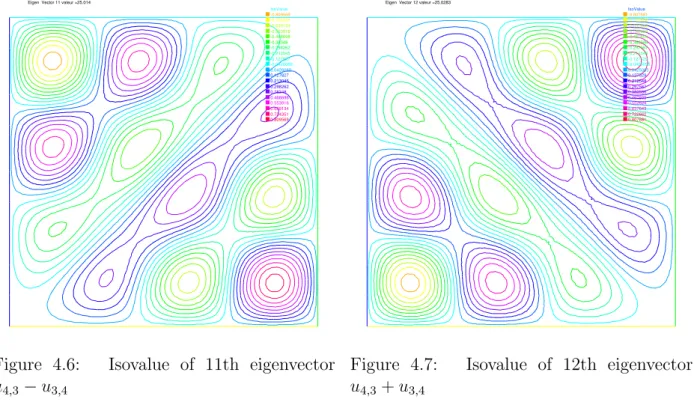
lambda[12]: 25.014 lambda[13]: 25.0283 lambda[14]: 26.0159 lambda[15]: 26.0159 lambda[16]: 29.0258 lambda[17]: 29.0273 lambda[18]: 32.0449 lambda[19]: 34.049 lambda[20]: 34.0492 - 0 5.0002 err= -0.000225891 - 1 8.00074 err= -0.000787446 - 2 10.0011 err= -0.00134596 - 3 10.0011 err= -0.00134619 - 4 13.002 err= -0.00227747 - 5 13.0039 err= -0.004179 - 6 17.0046 err= -0.00623649 - 7 17.0048 err= -0.00639952 - 8 18.0083 err= -0.00862954 - 9 20.0096 err= -0.0110483 - 10 20.0096 err= -0.0110696 - 11 25.014 err= -0.0154412 - 12 25.0283 err= -0.0291014 - 13 26.0159 err= -0.0218532 - 14 26.0159 err= -0.0218544 - 15 29.0258 err= -0.0311961 - 16 29.0273 err= -0.0326472 - 17 32.0449 err= -0.0457328 - 18 34.049 err= -0.0530978 - 19 34.0492 err= -0.0536275 ---IsoValue -0.809569 -0.724351 -0.639134 -0.553916 -0.468698 -0.38348 -0.298262 -0.213045 -0.127827 -0.0426089 0.0426089 0.127827 0.213045 0.298262 0.38348 0.468698 0.553916 0.639134 0.724351 0.809569 Eigen Vector 11 valeur =25.014

Figure 4.6: Isovalue of 11th eigenvector

u4,3−u3,4 IsoValue -0.807681 -0.722662 -0.637643 -0.552624 -0.467605 -0.382586 -0.297567 -0.212548 -0.127529 -0.0425095 0.0425095 0.127529 0.212548 0.297567 0.382586 0.467605 0.552624 0.637643 0.722662 0.807681 Eigen Vector 12 valeur =25.0283

Figure 4.7: Isovalue of 12th eigenvector

(45)

4.7. PLOT 45

4.7 Plot

With the command plot, meshes, isovalues and vector fields can be displayed.

The parameters of the plot command can be , meshes, FE functions , arrays of 2 FE functions, arrays of two arrays of double, to plot respectively mesh, isovalue, vector field, or curve defined by the two arrays of double.

The named parameter are

wait= boolean expression to wait or not (by default no wait). If true we wait for a keyboard up event or mouse event, the character event can be

+ to zoom in around the mouse cursor,

- to zoom out around the mouse cursor,

= to restore de initial graphics state,

c to decrease the vector arrow coef,

C to increase the vector arrow coef,

r to refresh the graphic window,

f to toggle the filling between isovalues,

b to toggle the black and white,

g to toggle to grey or color ,

v to toggle the plotting of value,

p to save to a postscript file,

? to show all actives keyboard char, to redraw, otherwise we continue.

ps= string expression to save the plot on postscript file

coef= the vector arrow coef between arrow unit and domain unit.

fill= to fill between isovalues.

cmm= string expression to write in the graphic window

value= to plot the value of isoline and the value of vector arrow.

aspectratio= boolean to be sure that the aspect ratio of plot is preserved or not.

bb= array of 2 array ( like [[0.1,0.2],[0.5,0.6]]), to set the bounding box and specify a partial view where the box defined by the two corner points [0.1,0.2] and [0.5,0.6].

nbiso= (int) sets the number of isovalues (20 by default)

nbarrow= (int) sets the number of colors of arrow values (20 by default)

How To Solve The Pde Problem On A Mesh With A Freefem++ (Freefemplest) On A Computer Or A Computer (For Freefems)

FreeFem++

Manual

http://www.freefem.org

http://www.ann.jussieu.fr/˜hecht/freefem++.htm

F. Hecht

, O. Pironneau

,

Universit´

e Pierre et Marie Curie,

Laboratoire Jacques-Louis Lions,

175 rue du Chevaleret ,PARIS XIII

K. Ohtsuka

,

Hiroshima Kokusai Gakuin University, Hiroshima, Japan

September 6, 2004

Contents

Chapter 1

Introduction

1.1

History

1.2

The language

1.3

Installation

Chapter 2

Syntax

2.1

Data Types

2.1.1

Another Example

2.2

List of major types

2.3

Globals

2.4

Arithmetic

2.5

Array

2.6

Loops

2.7

Input/Output

Chapter 3

Mesh Generation

3.1

Square

3.2

Border

3.3

Movemesh

---3.4

Reading and writing a mesh

3.5

Triangulate

3.6

Adaptmesh

3.7

Trunc

3.8

splitmesh

3.9

build empty mesh

3.10

Get Mesh numbering

3.11

Meshing examples

Chapter 4

Finite Elements

4.1

Problem and solve

4.2

Parameter Description for

solve

and

problem

4.3

Problem definition

4.4

Integrals