Introduction
In recent years there has been increasing interest in mac-roeconomic models of sectoral interlinkage in which com-modity price fl uctuation is put at the centre of all concerns. This concern is easily understandable, since fl uctuations in commodity prices induce fl uctuations in real national income and pose problems for macroeconomic manage-ment. These models have been seen as a way to formulate policy guidelines to reduce these fl uctuations. A key ele-ment in many of these models is overshooting of agricul-tural prices1 caused by unanticipated monetary expansion.
The point is obvious. If a stock of primary good is an asset and its price adjusts instantaneously, while industrial price adjusts slowly, agricultural price overshoots in response to monetary expansion.
The academic interest in the possible impacts of mone-tary policy on agricultural markets is of recent origin. Fran-kel (1986) set up a closed economy model to explain over-shooting of agricultural prices following an unanticipated expansion in money stock. He emphasised the distinction between fi xed price sectors (manufacturing), where prices adjust slowly and a fl ex price sector (agriculture), where prices adjust instantaneously in response to a change in the money supply2. Lai et al. (1996) employed Frankel’s
frame-work to investigate how anticipated and unanticipated mon-etary shocks infl uence commodity prices. Moutos and Vines (1992) also examined the role of commodity prices in the macroeconomic process of output and infl ation determina-tion. The econometric models of Orden and Fackler (1989) and Ghironi (2000) show that an increase in money supply raises agricultural prices relative to the general price level for more than a year, indicating persistence of the effect of 1 Overshooting of prices is defi ned as a temporary change in its value beyond its long run equilibrium.
2 Frankel’s model can be seen as an application of Dornbusch’s model of exchange rate dynamics.
monetary changes on relative agricultural prices both in the short run and in the long run. Saghaian et al. (2002) also explained short run and long run effects on agricul-tural prices in response to unanticipated monetary shocks. Bakucs and Fertő (2005) tested the overshooting hypothesis with reference to Hungarian agricultural prices. Saghaian
et al. (2002) studied the overshooting of agricultural prices in four Asian countries (Korea, Philippines, Thailand and Indonesia).
Once we get a story of commodity price fl uctuations, however, there arise some immediate questions. Is this
fl uctuation solely attributable to monetary shock? Do the existing monetary macro models provide an appropriate framework to predict commodity prices and more generally terms of trade behaviour? And, what are the macroeconomic implications of fl uctuations in terms of unemployment and output?
We develop a monetary macro model specially designed for a developing country. In particular, this paper makes a theoretical attempt to fi nd answers to these questions. Firstly, we introduce the medium term dynamics through adjust-ment of capital stock3. Secondly, the paper addresses the
issue of unemployment of industrial labour. In the model of the existing literature, full employment of labour is assumed and money is neutral in the long run. On the contrary, we incorporate unemployment through wage indexation. Spe-cifi cally, we assume that industrial wages are indexed to the consumer price index. Thirdly, the paper pays explicit atten-tion to both monetary and real shocks as sources of volatility of terms of trade. The model in this paper is a structuralist 3 There exists a literature on the medium-term adjustment in a dual economy. Car-doso (1981) applied a dual economy framework to capture the relationship between agricultural infl ation and wage formation. The dynamics in the Cardoso model are located in structural disequilibrium, namely the mismatch between wage goods con-straint and non-fulfi lment of aspirations of different groups. Taylor (1985) extended the model to include the capital accumulation process in an analysis of steady-state dynamics. Rattsø (1989) offered a similar investigation of the medium-run dynamics for a dual economy. However, these works left aside the role of speculation in inducing volatility in agricultural price.
Jonaki SENGUPTA*, Ranjanendra Narayan NAG** and Bhaskar GOSWAMI‡
Terms of trade, capital accumulation and the macro-economy in a
developing country: a theoretical analysis
This paper attempts to explain the terms of trade adjustment and the process of capital accumulation in a monetary model of sectoral interlinkage under rational expectation. The paper utilises a very standard dual economy framework in which industry and agriculture are two distinct sectors of production. Agriculture production is supply constrained. This may arise due to fi xed endowment of land, weather condition etc. On the other hand, employment and output in the industrial sector are determined on the basis of profi t maximisation in the presence of wage indexation. The asset structure of the economy includes the stock of primary commodities as one form of asset holding. Since the stock of agricultural commodities is one of the fi nancial assets, its demand is subject to speculation which may entail fl uctuating agricultural prices. Many factors have effects on fl uctuating agricultural prices. These include monetary shock, parametric changes in agricultural production, changes in government expenditure etc. In this paper we discuss the comparative static effects of parametric changes of these factors. The paper shows that the short run and long run effects of any particular shock are quite different, not only quantitatively, but also quali-tatively. Accordingly, the policy message of the paper is that the short run response may not be a reliable guide to the design of policy.
Keywords: industry-agriculture interlinkage, capital accumulation, terms of trade dynamics
* Charuchandra College, Kolkata, India.
** St. Xavier’s College (Autonomous), Kolkata, India.
monetary model focusing on terms of trade volatility, capi-tal accumulation, employment and output determination in the industrial sector under rational expectation and supply constraints imposed by the agricultural sector. Our model is more complex than the existing models due to two major modifi cations which are prompted by structural features in a developing country, namely unemployment and medium term dynamics through capital accumulation.
The paper is organised as follows. In the next section we build up the model and then we examine dynamic adjustment and examine saddle path stability of the system. Considera-tion of a few comparative static exercises follows, while the
fi nal section concludes the paper.
The model
Here we attempt to develop a monetary macro model of sectoral interlinkage. The model combines elements from recent research on commodity price fl uctuations in a rational expectation framework with (somewhat old) structuralist macroeconomic models of sectoral interlinkage in a dual economy structure. We integrate dual economy interlinkage in a developing country with full stochastic rational expecta-tions equilibrium in a monetary framework. Such integration and use of the model to study the macroeconomic implica-tions of commodity price fl uctuations induced by a variety of shocks are the purposes of this paper.
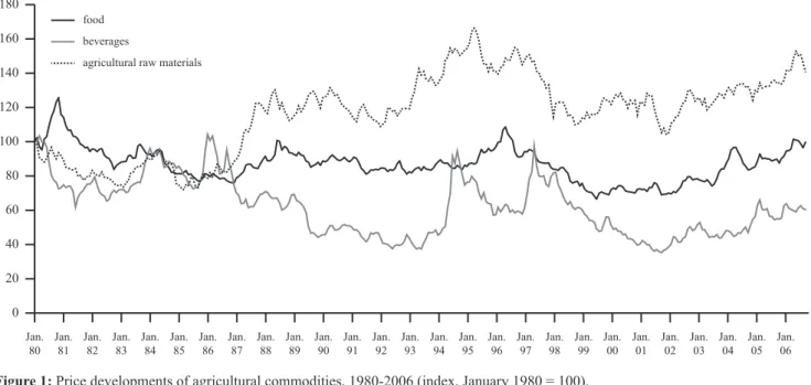
The goods produced are manufactures (produced in the industrial sector) and primary commodities (produced in the agricultural sector). We assume wage indexation for industrial workers, which allows for unemployment in the economy. Food price is a jump variable, which instantane-ously guarantees asset market equilibrium. In fact, prices of many agricultural commodities show a high degree of vola-tility caused by time lags between production decisions and delivery to the market; delayed and inappropriate responses by producers to price signals; inelastic supply and natural
shocks. This volatility aspect of commodity prices is evident from Figure 1.
Furthermore, the contribution of surging prices of pri-mary commodities in overall infl ation is quite substantial for developing countries compared to the advanced countries (Figure 2).
On the other hand, industrial price is sticky which leads to disequilibrium in the market for industrial goods. Moreo-ver, we assume that the economy is closed. Thus, the model in this paper is a disequilibrium, dual economy model with unemployment and perfect foresight.
This section is subdivided into three subsections. The fi rst contains a description of the supply side and this is followed by a description of asset structure with portfolio choice. The demand side is analysed in the third subsection along with an infl ation mechanism for industrial goods.
Figure 2: Contribution of food to headline infl ation.
Source: Loungani (2012) 180 160 140 120 100 80 60 40 20 0 Jan. 80 Jan. 81 Jan. 82 Jan. 83 Jan. 84 Jan. 85 Jan. 86 Jan. 87 Jan. 88 Jan. 89 Jan. 90 Jan. 91 Jan. 92 Jan. 93 Jan. 94 Jan. 95 Jan. 96 Jan. 97 Jan. 98 Jan. 99 Jan. 00 Jan. 01 Jan. 02 Jan. 03 Jan. 04 Jan. 05 Jan. 06 food
agricultural raw materials beverages
Figure 1: Price developments of agricultural commodities, 1980-2006 (index, January 1980 = 100).
The supply side
Agricultural output: Agricultural output (F) is fi xed in the time frame of our model4. Thus, we get the following
supply function of the agricultural output:
(1)
Industrial output:Labour (L) and capital (K) are used to produce the industrial output (Y). The production function for industrial production takes the following form:
(2) Employment in the industrial sector is derived from the condition of profi t maximisation, namely equality between marginal product of labour and real product wage. Thus we get the labour demand function as:
(3) where W is the money wage and PY is the price of industrial output.
Next we consider money wage determination. Instead of assuming fl exible adjustment in money wage, we take money wage to be determined as an outcome of a bargaining process. Specifi cally, we assume that money wage is deter-mined by a social pact which protects the real consumption wage. In other words, money wage is linked to the consumer price index:
(4) where α and 1–α are constant expenditure shares of indus-trial goods and agricultural goods respectively and PF is the price of agricultural output.
Now, (5)
where , is the terms of trade.
From equations (1), (3) and (5) we get the supply func-tion of industrial goods:
with
Aggregate output:Let Z denote aggregate output (or real income) measured in units of industrial goods:
(6)
4 Availability of land emerges as a binding constraint on agricultural growth. The potential of further expansion of the net sown area is practically non-existent and, given the environmental commitments, it may further decline. Moreover, a feeble price response is attributable not only to a reasonably fi xed land supply, but also to lower ini-tial input intensity and crop pattern governed by agro-climatic factors. One can intro-duce capital accumulation for the agricultural sector as well. However, agriculture in most developing countries has not experienced any major surge in private investment. In any case, industrial investment occurs more quickly and at a faster rate, compared to investment in the agricultural sector.
In what follows we take 5
The fi nancial sector
In the conventional dual economy models, food price equates to the fl ow supply and fl ow demand for agricultural output. Here, by contrast, we focus on the role of stock of primary goods as fi nancial assets and we study the effect of forward-looking food price expectation6. We assume that
stocks of food grains and government bonds are perfect sub-stitutes. The fi nancial sector is represented by the following equations:
(7) (8) where s is the difference between the convenience yield and the storage cost of holding primary commodities and is taken to be positive.
Equation (7) represents the money market equilibrium where M is the nominal money balance, which is defl ated by the price of manufactured goods. We choose a linear money demand function where demand for the real balance depends negatively on the interest rate and positively on real income.
Unlike manufactured goods, primary commodities are used as one form of asset along with money and bonds. Equation (8) refl ects the assumption of perfect substitutabil-ity between stocks of primary commodities and bonds such that returns on these two assets are brought into equality through arbitrage. The term represents expected change (and actual change under the assumption of perfect foresight) in food price. Hence, return on stocks of primary commodi-ties is ( ). The return on bonds is the interest rate (r)7.
Demand side and industrial price infl ation
We choose a linear consumption function such that total private consumption expenditure is C = βZ, where β is the marginal propensity to consume. Since α is the constant share of expenditure on industrial goods, the consumption demand for industrial goods is αβZ. Investment expenditure on the industrial goods depends on the real interest rate (r – πy ) where r is the nominal interest rate and π is the industrial infl ation rate and we choose a linear investment function, namely a – v(r –π) (a >0, v >0). Government expenditure (G) 5 The response of Z in response to θ is calculated as follows:
where eL is the elasticity of demand for labour in the industrial sector.
Clearly,
This condition is more likely to be satisfi ed in a dual economy with a signifi cant share of agricultural output in national income.
6 We note that the price of manufactured goods is used as the defl ator to express real income measured in units of industrial goods. However the model abstracts from adjust-ment in the stock of agricultural goods. Though this is a limitation of the model, this is a purposive abstraction which we make to keep the model within tractable limits. The similar abstraction is also made by Frankel (1986) and Moutos and Vines (1992). 7 Thus we use an asset approach to examine food price dynamics.
is parametrically given. Thus the aggregate demand for the industrial goods is (αβZ + a – v(r – π) + G).
Next, we consider infl ation dynamics. Instead of allow-ing instantaneous market clearallow-ing of industrial goods, we assume the industrial price to be sticky. However, the infl a-tion rate can change in response to excess demand for the industrial goods. Now a few comments on the industrial price are in order. Since the price of industrial goods cannot jump, the industrial sector can remain in disequilibrium. The form of disequilibrium determines the infl ation rate. Thus, the cur-rent industrial price level is determined by the past rates of infl ation and the current infl ation rate determines the future price level. At any particular point in time the industrial price is predetermined. Now the infl ation rate of industrial price is:
(9)
Dynamic adjustment and stability
Firstly we consider dynamic adjustment of the terms of trade. Equations (8) and (9) can be combined together to pro-duce the dynamic adjustment in the terms of trade. Noting
that , we get:
(10) In an implicit form the terms of trade dynamics can be expressed as:
(11) with g1>0, g2>0, g3>0, g4<0, g5<0 where:
and we assume that food price infl ation is greater than indus-trial price infl ation and A is a constant.
and we assume that food price infl ation is greater than indus-trial price infl ation.
The intuitive explanation of sign restrictions are as fol-lows:
We begin with an initial steady state value θ such that and examine the effect on following any change in variables that appear in equation 11. A rise in θ leads to an increase in the real income and hence the demand for money
goes up which leads to an increase in interest rate and causes food price infl ation. This follows from equations (7) and (8). On the other hand, a rise in θ leads to a fall in the industrial output. On the demand side, private consumption expendi-ture on industrial good rises, but private investment falls. For reasonably low interest elasticity of private investment, we can assume that there is an increase in the excess demand for industrial goods and a consequent increase in the rate of industrial price infl ation. However, we assume that the rate of food price infl ation exceeds that of industrial price infl a-tion in response to the rise in θ such that g1 > 0.
Next, we consider a rise in K. This causes industrial output to rise. Since aggregate income rises for any given value of θ, the interest rate rises to maintain money market equilibrium, which leads to food price infl ation (this follows from equation 8).
On the other hand, a rise in the industrial output and fall in investment reduce the rate of industrial price infl ation. Hence, g2 > 0. Now, a rise in F increases the real income, which causes interest rate to rise. As a result the rate of food price infl ation increases. However, the effect on the infl ation rate of industrial price is ambiguous. On the one hand, we have an increase in consumption expenditure on the industrial output and on the other we have a fall in investment expendi-ture. However, we assume that the rise in food price infl ation exceeds any possible increase in the rate of industrial price infl ation such that g3 > 0. The explanation for g4 < 0 is sim-ple. A rise in government expenditure increases the rate of industrial price infl ation and hence makes , i.e. g4 < 0.
Lastly, we consider the effect of increase in money sup-ply on . A rise in money supsup-ply entails a fall in the interest rate such that the rate of food price infl ation falls and a rise in investment leads to an increase in the rate of industrial price infl ation. This leads to , i.e. g5 < 0.
Next, we consider the dynamics of capital accumulation. Beyond the short run, investment alters the size of the
capi-tal stock: , where δ is the
rate of depreciation and is positively related to the stock of industrial capital. In an implicit form, the dynamics of capi-tal accumulation can be expressed as:
(12) With the following restrictions on the signs of partial
derivatives: .
Intuitive explanations for these sign restrictions are as follows:
and hence reduce investment, while a rise in M leads to a fall in the interest rate and hence a rise in investment.
In the steady state and
The slope of is and the slope of
is
Equations (11) and (12) constitute a system of differen-tial equations in the terms of trade and the capital stock. The terms of trade is free to jump in response to news, which includes unanticipated current and future changes in exog-enous variables and policy instruments. However, the capi-tal stock in the industrial sector is a predetermined variable which can change only on a fl ow basis in response to invest-ment. We concentrate on a stable saddle path because it gives an economically meaningful result. In the presence of per-fect foresight the existence of a unique convergent saddle path requires that there must be one positive and one nega-tive characteristic root such that the determinant:
This condition is satisfi ed if the locus is steeper than the locus (Figure 3). The saddle path SS is down-ward sloping and fl atter than the locus. The equation of the saddle path is
Comparative statics
In this section we consider the effect on terms of trade and capital stock in response to a variety of shocks. The specifi c shocks examined are: (a) increase in money supply, (b) increase in government expenditure and (c) a rise in the agricultural output of food.
Monetary expansion
In our model the real money supply in units of industrial goods is fi xed. Thus money supply adjusts in response to infl ation of industrial goods. In other words, money supply is proportional to the price of industrial goods. By monetary policy we mean change in this proportion8. An increase in
real money balance may generate a contractionary effect on industrial output along with industrial price infl ation. The explanation of the effect of monetary expansion is straight-forward.
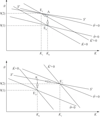
Let us consider an increase in real balance. This leads to a fall in the interest rate and hence it causes a fall in the rate of food price infl ation. Again, private investment rises due to the fall in the interest rate, which entails a rise in the rate of industrial price infl ation. On both counts, we have a fall in the rate of change in θ, that is, we have , starting
from . Hence, θ will rise to maintain . This is
represented by an upward shift of the curve. Since
interest rate falls, private investment rises and the curve shifts to the right. For any given value of the stock of industrial capital, the terms of trade increases leading to a rise in the real wage rate and a consequent fall in the indus-trial output. A possible long run outcome is a fall in the stock of industrial capital at the end the adjustment process. In the case of a fall in the capital stock, the terms of trade undershoots its long run equilibrium value. This will exac-erbate the initial industrial recession. On the other hand, if capital stock increases, terms of trade overshoots in the long run (Figures 4a and 4b).
8 We consider the cases where monetary changes are both unanticipated and imple-mented as soon as they are announced.
ș(2) ș K K1 K0 ș(1) S' E1 A E0 S' K'=0 K=0 ș /=0 ș=0 ș(1) ș K K1 K0 ș(2) S' E / 1 A/ E / 0 S' K'=0 K=0 ș /=0 ș=0
Figure 4: (a) Undershooting and (b) overshooting of θ associated
with monetary expansion.
Source: own composition
ș K K=0 ș=0 S S
Figure 3: Phase diagram and saddle path stability with θ being the
jump variable and K being the slow moving variable.
In Figure 4a (4b) the equilibrium initially jumps from point E0 ( ) to point A (A/) along the new saddle path. Since K cannot jump instantaneously, point A (A/) is the only
tran-sitional position. The transition towards the new steady state is characterised by the path between A (A/) and E
1 ( ), along
which K declines (rises) and θ increases. In fact, a decrease (increase) in K causes a rise (fall) in θ causing undershooting of θ. The fi nal and initial changes in θare represented by fol-lowing two equations respectively:
The initial change in θ is given by:
Subtracting the second equation from the fi rst equation we obtain the value of undershooting or overshooting of θ
and this is given by:
If α1 > 0 i.e. capital stock increases, then the terms of trade overshoots. On the other hand, if α1 < 0 i.e. capital stock decreases the terms of trade undershoots9.
Rise in government expenditure
An increase in government spending on manufactured goods leads to a rise in the rate of industrial price infl ation.
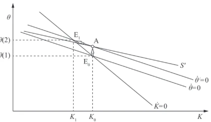
This in turn causes , starting from . Thus fi scal
expansion shifts the curve upwards. For any given
value of the stock of industrial capital, the terms of trade rises on impact and the economy is placed at point A. Over a period of time the capital stock begins to decline and the terms of trade rises further. Thus, the model shows under-shooting of the terms of trade following fi scal expansion. The rise in terms of trade causes an initial contraction of the industrial sector, which is aggravated by a fall in the capital stock.
Our result needs to be contrasted with the general price overshooting model (Frankel, 1986; Moutos and Vines, 1992). In those papers, there was an unambiguous expansion of industrial output and an ambiguous effect on the terms of trade. Moreover, in their papers the terms of trade may either overshoot or undershoot. In our model, the terms of trade unambiguously move in favour of the agricultural sector and, given wage indexation in the industrial sector, a rise in the terms of trade invariably leads to a fall in industrial out-put. Moreover, capital stock decumulation in the industrial sector causes undershooting of the terms of trade.
This is illustrated in Figure 5 where the equilibrium ini-tially jumps from point E0 to point A along the new saddle path. Since K cannot jump instantaneously, point A is the only transitional position. The transition towards the new steady state is characterised by the path between A and E1 along which K declines and θ increases. In fact, a decrease 9 See the mathematical appendix for derivation of both steady state effects and tran-sitional dynamics.
in K causes a rise in θ causing undershooting of θ. The initial and fi nal changes in θ can be captured by following equa-tions:
The initial change in θ is given by:
Subtracting the second equation from the fi rst equation we obtain the value of undershooting of θ and this is given by:
Since α3 < 0 i.e. capital stock decreases, the terms of trade undershoots.10
Rise in agricultural output and relaxation of supply constraint
Rising agricultural production is of great importance in promoting economic development. Since land is a major constraint, agricultural expansion requires signifi cant tech-nological progress. In this paper a rise in agricultural output may lead to an expansion in industrial output. This is amena-ble to easy economic interpretation.
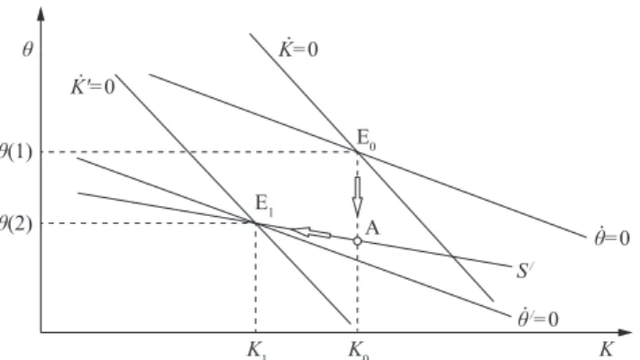
Suppose we consider an increase in agricultural output. This leads to an increase in aggregate income and hence the demand for money rises. It follows from the money market equilibrium the interest rate rises, leading to . On the other hand, the effect on excess demand for the industrial output is ambiguous. It has already been explained in the
context of dynamic adjustment of the system,
follow-ing an increase in the agricultural output. Hence, the curve shifts downwards (Figure 6). Again, a rise in interest 10 Long run and transitional dynamics of fi scal expansion can be calculated very eas-ily by similar methods as in increase in money supply.
ș(1) ș K K1 K0 ș(2) E1 E0 A S' K=0 ș/=0 ș=0
Figure 5: Undershooting of θ on account of a rise in government
expenditure.
rate reduces investment and the shifts to the left. The effect on the stock of industrial capital is ambiguous. In case of a rise (fall) in the stock of industrial capital the terms of trade undershoots (overshoots) its long run equilibrium value. However, it is unambiguous that the terms of trade decline on impact, leading to an expansion of industrial out-put. The fi nal effect on industrial output is, however, ambig-uous. If the stock of industrial capital rises, the initial favour-able effect on the industrial output is reinforced. In the case of a decline in the industrial capital the initial effect may be short-lived and industrial recession may follow, despite an increase in the agricultural output.
The fi nal change in θ can be given as:
The initial change in θ is given by:
Subtracting the second equation from the fi rst equation we obtain the value of undershooting or overshooting of θ
and this is given by:
If α6 < 0 i.e. capital stock decreases, then the terms of trade undershoots. On the other hand, if α6 < 0 i.e. capital stock increases, then the terms of trade overshoots.
Discussion
In this paper we have examined the role of commod-ity prices in shaping the macroeconomic process of output, infl ation and terms of trade determination. Our aim has been to show the important role which commodity prices can play in overall macroeconomic developments. The short run and long run impacts of different macroeconomic policy add to price and income instability, and infl uence fi nancial viability of farmers tremendously.
The empirical relevance of such a model is also very robust. But we depart from these existing literatures in terms of two fundamental differences in the characterisation of
a dual economy. The specifi c features of the model in this paper are completely suitable for a developing economy. One basic difference is the nature of determination of indus-trial output. The paper addresses the issue of unemployment of industrial labour. In the existing literature, most of the models assume full employment of labour and accordingly these models obtain long run neutrality of money. We depart from the existing literature in the sense that we incorporate unemployment through wage indexation.
The second difference is the medium run adjustment through the process of accumulation of industrial capital, which our paper focuses on. All medium run macro mod-els are non-monetary macro modmod-els. On the other hand, the existing monetary macro models which explain the volatil-ity of agricultural price is typically a short-run model in the sense that adjustment in capital stock is ignored. We try to integrate both approaches by incorporating adjustment of capital stock in a monetary, dual economy framework. The adjustment in the stock of industrial capital also leads to a difference in the short run and the long run effects of differ-ent macroeconomic shocks.
One possible extension of the paper is to introduce open economy dimensions into the model. One can realistically assume that the agricultural sector produces not only for the home market but also for the external market, particularly in the post-WTO situation and the industrial sector uses an imported input. There is hardly any literature on dual economy interlinkage in an open economy, monetary macro model11. Clearly the content of our paper can be suitably
modifi ed to accommodate relevant open economy issues.
Mathematical appendix
Saddle path derivation
From equation (11) and (12) we can write:
(1) (2) Taking Taylor series linear approximation around the ini-tial steady state values for period t≤T,12 we get:
(3) (4) Arranging (3) and (4) in matrix form, we get:
(5) Similarly for period t≥T,13 we get:
(6) 11 Orden and Fackler (1989), Ghironi (2000), Saghaian et al. (2002), Nag end Gos-wami (2005) and Asfaha and Jooste (2007) develop an open economy macro model which examines the issue of volatility of agricultural price.
12 Here T denotes the time period at which a change in exogenous variable occurs. 13 Here t≥T, denotes the time period after a change in exogenous variable takes place. ș(2) ș K K1 K0 ș(1) E1 E0 A S/ K'=0 K=0 ș/=0 ș=0
Figure 6: Overshooting of θ associated with an increase in
agricultural output.
(7) The dynamics in period t≥T are specifi ed by
(8) Clearly eigen values λ1 and λ2 of equation 5 and 8 are identical. For the saddle path stability we require that
. Let us assume that λ1< 0, λ2> 0. Now, over the period 0 < t≤T, the solutions for K and θ
are given by
(9) (10) Again, for the period t≥T, the solutions for K and θ are:
(11) (12) It is noted that θ(t) and K(t) do not diverge as t→α when
and hence the solutions would be:
(13) (14)
The remaining constants are obtained by
solving the equations:
(15) (16) (17) Here dθ and dK are shifts in the steady state correspond-ing to particular shift parameter. Now the stable saddle paths after time T are described by equations (11) and (12).
Elimi-nating from these equations we get:
(18)
Comparative statics
Increase in money supply
Long run effects:
From equation (11) and (12) we get:
(11a) (12a) Differentiating equations (11a) and (12a) with respect to
M and setting and respectively we get:
(19) Applying Cramer’s Rule we get:
(20) (21)
Transitional details
To obtain the initial jump in θ after increase in M, we set
t = 0 and using A1 = –A2 in equation 10 we get:
(22) Solving equations (16) and (17) we get:
(23) Substituting the value of A2 in equation (22) we get:
(24) Equation (24) represents initial jump in θ.
The value of overshooting or undershooting of θ we sub-tracting equation 24 from equation 20 and this is given by
( is the fi nal steady state value of θ )
Since from the slope saddle path, we get
clearly undershooting of θ when capital stock decreases i.e.
α1< 0. On the other hand, if capital stock increases the terms of trade overshoots in the long run.
References
Asfaha, T.A. and Jooste, A. (2007): The Effect of Monetary Chang-es on Relative Agricultural PricChang-es. Agrekon 46 (4), 460-473. http://dx.doi.org/10.1080/03031853.2007.9523781
Bakucs, L.Z. and Fertő, I. (2005): Monetary Impacts and Over-shooting of Agricultural Prices in Transition Economy. Paper presented at the XIth International Congress of the EAAE, Co-penhagen, Denmark, 24-27 August 2005.
Böwer, U., Geis, A. and Winkler, A. (2007): Commodity price
fl uctuations and their impact on monetary and fi scal policies in Western and Central Africa. Occasional paper series no 60. Frankfurt am Main: ECB.
Cardoso, E.A. (1981): Food Supply and Infl ation. Journal of Devel-opment Economics 8,269-284.
Frankel, J.A. (1986): Expectations and Commodity Price Dynam-ics: The Overshooting Model. American Journal of Agricultural Economics 68 (2), 344-348. http://dx.doi.org/10.2307/1241436 Ghironi, F. (2000): Alternative Monetary Rules for a Small Open
Economy: The case of Canada. Boston College Working Papers in Economics No. 466. Chestnut Hill MA: Boston College. Lai, C., Hu, S. and Wang, V. (1996): Commodity Price
Dynam-ics and Anticipated Shocks: American Journal of Agricultural
Economics 78 (4), 982-990. http://dx.doi.org/10.2307/1243854 Loungani, P. (2012): Commodities Market: Developments and Out-look. PowerPoint® presentation [www document]. http://www.
imf.org/external/np/res/commod/pdf/CommoditiesMarket.pdf (accessed 24 September 2013).
Moutos, T. and Vines, D. (1992): Output, infl ation and commodity prices. Oxford Economic Papers 44 (3), 355-372.
Nag, R.N. and Goswami, B. (2005): Dual economy interlinkage in a monetary economy: A post WTO perspective. Journal of Eco-nomic Integration 20 (3), 497-513. http://dx.doi.org/10.11130/ jei.2005.20.3.497
Orden, D. and Fackler, D.L. (1989): Identifying Monetary Im-pacts on Agricultural Prices in Var Models. American Jour-nal of Agricultural Economics 71 (2). 495-502. http://dx.doi. org/10.2307/1241620
Rattsø, J. (1989): Macrodynamic Adjustment Mechanisms in a Dual Semi-Industrialised Economy. Journal of Develop-ment Economics 30, 47-69. http://dx.doi.org/10.1016/0304-3878(89)90050-3
Saghaian, S.H., Hasan, M.F. and Reed, M.R. (2002): Overshoot-ing of Agricultural Prices in Four Asian Economies. American Journal of Agricultural Economics 34 (1), 95-109.
Taylor, L. (1985): A Stagnationist Model of Economic Growth. Cambridge Journal of Economics 9, 383-405.