Consumer demand for meat in Finland

(1)

Consumer demand for meat in Finland

Johannes Piipponen Master`s thesis Agricultural Economics Department of Economics and management University of Helsinki September 2017

(2)

Faculty

Faculty of Agriculture and Forestry

Department

Department of Economics and Management

Author Johannes Piipponen

Title

Consumer demand for meat in Finland

Subject

Agricultural Economics

Level

Master’s thesis Month and year 9/2017

Number of pages 55+8 (Appendices)

Abstract

This paper focuses on meat consumption patterns in Finland. Empirical analysis for this paper was based on the micro data of three Household Budget Surveys: 1998, 2006 and 2012. A censored linear approximation of the almost ideal demand system (LA-AIDS) model was employed in the study. The major outcomes of the study were the demand expenditure and price elasticities that were obtained from the parameter estimates of five different meat products. Since the data lacked price information, unit values were used as a price substitutes, which gave some insights into quality-quantity upgrading.

According to the results, pork expenditure was elastic and thus was luxury good during the study period, whereas ruminant meat and poultry were luxuries only in 2000s. In addition, the price of a good, household size, and income had a large influence on meat consumption. Additionally, other factors (such as age) affected the portion of the budget that was allocated to meat products. In order to obtain more information relating to the food sector, further research concerning disaggregate demand would be needed.

Keywords

meat, demand elasticities, Almost Ideal Demand System, LA-AIDS

Where deposited

Helsinki University Library – Helda / E-thesis (Theses) ethesis.helsinki.fi

Further information

Supervisor: Xavier Irz, Natural Resources Institute Finland Reviewer: Antonios Rezitis, University of Helsinki

(3)

Tiedekunta/Osasto Maatalous-metsätieteellinen tiedekunta Laitos Taloustieteen laitos Tekijä Johannes Piipponen Työn nimi

Consumer demand for meat in Finland

Oppiaine Maatalousekonomia Työn laji Maisterintutkielma Aika 9/2017 Sivumäärä 55+8 (liitteet) Tiivistelmä

Vaikka kasvisten ja vaihtoehtoisten proteiinilähteiden arvellaan vähentävän lihatuotteiden suosiota, kasvava lihan kulutus ei näytä saavuttaneen lakipistettään. Terveysongelmien lisäksi korkea lihakulutustaso nähdään biodiversiteettiä heikentävänä ja kasvihuonekaasuja tuottavana ympäristön rasittajana. Kulutuksessa tapahtuviin muutoksiin ja muutosten aiheuttamiin vaikutuksiin ei voida reagoida tehokkaasti ellei kulutukseen vaikuttavia taustatekijöitä tunneta.

Tässä tutkimuksessa lihan kysyntää, ja siihen vaikuttavia tekijöitä analysoitiin ekonometristen menetelmien avulla. Lihatuotteet jaoteltiin ryhmiin (nauta ja lammas, sianliha, siipikarjanliha, prosessoitu liha, muut lihatuotteet) ja aineistona käytettiin Tilastokeskuksen kulutustutkimus-aineistoja vuosilta 1998, 2006 ja 2012. Tutkielman päätuotoksena ovat kysynnän hinta- ja menojoustot, jotka estimoitiin sensoroidun lineaarisen moniyhtälömallin (LA-AIDS) avulla. Joustot kertovat kuinka herkkiä eri lihatuotteet ovat hintavaihteluille ja paljastavat ryhmien välisiä tulo- ja substituutiovaikutuksia. Lisäksi tutkimustulokset kertoivat, kuinka sosio-ekonomiset muuttujat kuten tulotaso, koulutus ja ikääntyminen vaikuttavat kunkin liharyhmän kulutukseen.

Kulutus ohjaa koko ruokaketjun toimintaa; tuotantoa, tuontia ja vientiä. Jatkotutkimuksen tarvetta ja vastaavanlaisen analyysin laajentamista muille elintarvikesektoreille korostetaan.

Avainsanat

Liha, kysyntä, joustot, LA-AIDS

Säilytyspaikka

Helsingin yliopiston kirjasto – Helda / E-thesis (opinnäytteet) ethesis.helsinki.fi

Muita tietoja

Ohjaaja: Xavier Irz, Natural Resources Institute Finland Tarkastaja: Antonios Rezitis, University of Helsinki

(4)

Abbreviations list

AIDS Almost Ideal Demand System CDF Cumulative Density Function

COICOP Classification of individual consumption by purpose EASI Exact Affine Stone Index

FBS Food Balance Sheet HBS Household Budget Survey

ITSUR Iterative Seemingly Unrelated Regression

LA-AIDS Linear Approximation Almost Ideal Demand System LR Likelihood Ratio

PDF Probability Distribution Function

(5)

1 Introduction

1.1 Background and aims of the study

In recent years, the trends and patterns of food consumption have been a topic of much discussion. While the demand for vegetables and environmentally friendly food products has increased, meat consumption has simultaneously increased. This raises questions regarding consumer trends in meat consumption – are meat consumption levels nearing their saturation point? Or will meat consumption continue to increase from some time to come? (Vranken et al., 2014.)

Because livestock production has a notable impact on the decrease of biodiversity and increase of greenhouse gases, the reduction of high-level meat consumption is often seen as a clear way to decelerate climate change (Stoll-Kleemann and Schmidt, 2017). In Finland, this has a great effect on the food sector, as the food sector in Finland is heavily based on animal production. Additionally, excessive meat consumption can increase the risk of developing certain health problems. Although decreasing meat consumption could be achieved by restricting the choices of consumers (Lombardini and Lankoski, 2013), taxation of meat products is considered to be a more effective method (Nordgren, 2012).

It is public knowledge that food consumption habits are driven by a multitude of factors including, but not limited to: income, age, economic status, price fluctuations, nutritional trends, etc. The degrees to which these various factors affect consumptions patterns, however, are less clear. From a political standpoint, numerical data relating to the amount of impact that each of these factors has on the consumption levels of food products would be very valuable. For example, Vinnari (2008) speculates that an increased taxation of meat products could effectively reduce meat consumption in Finland, but without concrete numerical data regarding the demand elasticity of meat products after increased taxation, Vinnari’s speculation is just that – speculation. Attempts to guide consumer habits without a basis in consumer research are likely to prove ineffective.

Most recent studies pertaining to the demand for meat products (where household-level data is utilized) were done in Africa (Aborisade et al., 2017; Delport et al., 2017; Shibia et al., 2017) and in France (Dahlberg, 2017a). In Finland, this type of research has mostly been performed using Household Budget Survey data and has concentrated

(7)

on a more general food spectrum; research relating to a more specific food category (e.g. meat) does not exist. The first demand system approach to this type of research in Finland was conducted by Laurila (1994), followed by Irz (2017), who published a comprehensive demand analysis article where food consumption was aggregated into 19 categories. This means, of course, that the meat sector has also been extensively researched; however, a quantitative analysis that explains the drivers affecting changes in consumptive trends within the meat industry has yet to be performed. This study will investigate factors that affect household demands for meat products and will attempt to create a basis for future studies pertaining to this topic.

The main outcomes are demand elasticities, which provide information about the necessity of a food product – that is, it predicts the amount that demand for a certain commodity will fluctuate if the price of said product rises. Without an adequate understanding of the dynamics surrounding supply and demand in relation to the price of a product, it is impossible to enact effective policies for promoting or reducing the consumption of a certain product – the repercussions of such blind policymaking are far too uncertain.

After a general view of meat consumption is presented, common consumer theory is examined in Chapter 2 as well as the model used in this study. Chapter 3 examines the Household Budget Survey (HBS) data, describes preparations and corrections that must be made before estimation, and provides summary tables concerning variables defined in HBS. The estimation process is explained in Chapter 4, and Chapter 5 expresses and interprets the outcome of the estimation process. Chapter 6 contains the final summary of this thesis and recommends topics for future studies related to this study. This thesis is part of the RUOMU project at the Natural Resource Institute of Finland. This project produces information regarding the structure of Finnish food markets as well as the competitiveness and efficiency of the food sector in Finland.

(8)

1.2 Survey of meat consumption in Finland

According to national data provided by Statistics Finland (2017), private consumption expenditure for meat and meat products has increased by over 60 per cent from 1975 to 2015 when measured using reference prices from 2010. During the same time period, meat consumption per person has increased by almost 30 per cent, with the average being over 80 kilograms per person in 2016 according to Food Balance Sheets (Luke, 2017a). These changes are presented in graph form below (Figure 1; Figure 2). Although all classifications differ between the Food Balance Sheet (FBS) and national accounts, some observations can be made. In the 2000s, there is no clear sign that consumption levels of any meat product would obviously be falling, whereas rapid growth in poultry consumption is apparent. Beef and pork consumption remains stable, but, according to national accounts, the consumption of tinned and processed meat products is becoming more common. It is worth mentioning that the HBS covers only food consumed at home, while the FBS contains all food. In fact, just the inclusion of food consumed away from home may explain the divergence between HBS and FBS trends.

Figure 1. Meat consumption expenditure 1975-2015 at reference year 2010 prices (Statistics Finland, 2017)

(9)

Figure 2. Meat consumption in Finland according to Food Balance Sheets (Luke, 2017b)

In spite of tremendous growth, the consumption of meat in Finland is still below the average consumption levels in the EU-area (Figure 3). In some countries meat consumption has exceeded 100 kilograms, which leads one to believe that an increase in meat consumption in Finland is still possible. The importance of meat consumption analysis cannot be undervalued, as intentions to reduce meat production will only provoke more discussion in the future. This will have a direct impact on the production, import, and export of meat products in Finland.

Figure 3. Meat consumption in selected EU countries in 2016. (TNS Gallup, 2017)

0 20 40 60 80 100 120 kg/cap ita /y ear

(10)

2 Theoretical Background

2.1 Consumer theory

This study will be utilizing an empirical model that is based on common consumer theory, which was explained in detail by Varian (2014). Classical micro theory attempts to explain consumer rationality by applying a set of rules to the thought processes that the consumer goes through when a purchase is being made. More specifically, the axioms considered in this definition of the consumer thought process are: completeness, transitivity, continuity, and monotonicity. The completeness axiom operates under the assumption that the consumer is always able to choose between two goods and determine which of those two goods is of equal or superior quality. The transitivity aspect considered when applying these rules assumes the consumer rationality that: if A is preferred to B, and B is preferred to C, then A is also preferred to C. The continuity axiom makes the application of the utility function possible, as continuity does not allow the possibility of open sets. Finally, monotonicity is based on the given that goods are desirable to the consumer, and can be explained simply using the phrase “more is better than less” – that is having more of a certain good is definitely better than having less of said good. (Varian, 2014.)

Now that the basic principles of consumer theory are understood, it is important to examine the functions used in analyzing cost and utility, as these are two of the key components that will be applied when using the demand system model. Consumers tend to maximize product utility in relation to their expenditure limitations (primal problem) and will react rationally to changes in this formula. The utility maximization or the primal problem can be defined as follows:

(1) max 𝑢 = 𝑣(𝑞), 𝑠. 𝑡. 𝑝𝑞 = 𝑥,

where v(q) denotes utility, q is a vector of quantities consumed, p is a corresponding price vector and x a is fixed budget. As an alternative to utility maximization, consumers can minimize their expenditure for a given utility level (dual problem): (2) min 𝑥 = 𝑝𝑞 , 𝑠. 𝑡. 𝑣(𝑞) = 𝑢

The primal and dual problems lead to Marshallian and Hicksian demand functions respectively. Furthermore, we can derive the indirect utility function as well as the expenditure function from these demand functions as they are closely interrelated

(11)

through the Slutsky equation. (Edgerton et al., 1996.) The demand systems presented later are based on these properties. The closer examination and derivation of these functions is presented in Deaton and Muellbauer (1980a, 1980b).

2.2 Theoretical restrictions of the demand models

There are some restrictions that must be implemented in demand models, as estimations without them are not consistent with theory. These restrictions control the parameters estimated from Marshallian demand equations. However, these restrictions are often violated in practice, which decreases the credibility of the obtained results (Deaton and Muellbauer, 1980a). Also, the restrictions have to be tested, as they are worthless otherwise (Shukur, 2002). In this section, information regarding these restrictions is presented generally, but restrictions linked to parameter estimation and testing procedures will be discussed in more depth in Chapter 4. The following definitions are based on the findings of Deaton and Muellbauer (1980b) and Edgerton et al. (1996).

The first frequently imposed restriction that must be discussed is adding-up, which means that sum of the Marshallian demand functions must result in total consumption. In other words, the consumer’s budget must be totally used. The adding-up restriction is the result of the budget constraint and monotonicity assumptions. The second restriction, homogeneity, suggests an absence of money illusion, in which case only the relation between prices and the total budget is significant. Under these circumstances, even if we change the prices and expenditures proportionally in the primal problem (1), neither the utility function nor budget constraint will be changed. The third restriction is symmetry (Slutsky symmetry), which ensures consumer rationality. The symmetry property is linked to substitution matrices and derivatives of demand functions. The fourth, and most rarely observed property, is negativity. As the expenditure function is concave regarding prices, the substitution matrix is negative and semidefinite, and the diagonal elements of the matrix are negative as well. This restriction can be tested only after other calculations have been performed. While adding-up and homogeneity are required to satisfy the budget constraint, symmetry and negativity allow for utility maximization. Usually the homogeneity and symmetry properties are imposed on the demand model as they do not cause severe estimation difficulties, and their validity is easy to test.

(12)

2.3 Almost Ideal Demand System (AIDS)

The consumer theory gives guidelines for selecting functional form for empirical analysis of demand. Many functional forms have been proposed as alternatives for demand analysis tools. The first of these was developed in the 1950s, when Stone suggested his linear expenditure system (LES) that was derived from classical micro theory (Stone, 1954). Following the model presented by Stone, the Rotterdam model (Barten and Theil, 1964-1965) and the translog model (Christensen et al., 1975) rose in popularity as a marketing research tool until 1980, when the Almost Ideal Demand System (AIDS) was developed by Deaton and Muellbauer. Finally, as alternative to the AIDS model, the Exact Affine Stone Index (EASI) was suggested in 2007. (Clements and Selvanathan, 1988; Lewbel and Pendakur, 2007.)

Over the time the models became more flexible and later systems had advantages over older ones (Deaton and Muellbauer, 1980a). Nowadays different price indices and linear or non-linear approximations specify the models further and there is not mutual understanding which combination of these would produce most reliable results (Barnett and Serletis, 2008). Since the AIDS model is most commonly used in demand system analysis, it will be used in present study.

The AIDS model was created by Deaton and Muellbauer in 1980, and has since been the preferred method for product demand analysis, due to its flexibility and compatibility with household-level data. (Delport et al., 2017). The AIDS model satisfies the axioms of choice, aggregates over consumers and gives first-order approximation to any demand system. Also, as the homogeneity and symmetry depend only on the estimated parameters, these restrictions are easy to impose and test. Thus, the AIDS model has several desirable properties, some of which are missing from preliminary demand systems. The AIDS based on revealed preferences, which are often considered superior compared to stated preferences. (Deaton and Muellbauer, 1980a; Irz, 2017.)

The model consists of various demand functions that are used to calculate the correlation coefficient between the budget shares of different commodities, relative product prices, and total consumer expenditures (Lewbel and Pendakur, 2007). The AIDS model is derived from PIGLOG class cost function by using Shephard`s lemma

(13)

and budget share functions are linear in parameters. Deaton and Muellbauer (1980) presented the basic form of the AIDS model as (3):

(3) 𝑤_𝑖ℎ = 𝛼_𝑖+ ∑ 𝛾_𝑖𝑗 𝑛

𝑗=1

𝑙𝑛𝑃_𝑗+ 𝛽_𝑖ln (𝑋ℎ

𝑃_ℎ) + 𝑢𝑖ℎ , 𝑤ℎ𝑒𝑟𝑒

• 𝑤_𝑖 is the expenditure share allocated to ith good (defined by 𝑤_𝑖 =𝑃𝑖𝑄𝑖

𝑋 ) in

household h

• 𝑃_𝑗 is the price of jth good

• 𝑋ℎ is the total expenditures in household h

• 𝛼𝑖 , 𝛾𝑖𝑗 𝑎𝑛𝑑 𝛽𝑖 are parameters to be estimated, 𝑢𝑖ℎis the random error

term

• 𝑃_ℎ is a translog price index (defined in Appendix)

However the nature of the translog price index makes the model non-linear, which causes empirical problems – especially with aggregated data. By replacing price index P with Stone`s price index P* the AIDS model can be linearized (Deaton and Muellbauer, 1980a; Green and Alston, 1990). This linear form is known as the Linear Approximation Almost Ideal Demand System (LA –AIDS). Formation of the model used in the study as well as Stone and translog price indices are presented in the Appendix.

Many researchers consider LA-AIDS model more suitable and easily estimated than traditional AIDS. For example Abodisade et al. (2017), Delport et al. (2017), Green and Alston (1990), Shibia et al. (2017) to name a few. Also in my thesis the LA-AIDS model is being used. Theoretical restrictions on the parameters of the LA-AIDS model include adding-up (4), homogeneity (5), and symmetry (6).

(4) ∑ 𝛼𝑖 = 1 𝑛 𝑖 ∑ 𝛽𝑖 = 0 𝑛 𝑖=1 ∑ 𝛾𝑖𝑗 = 0 𝑛 𝑖=1 (5) ∑ 𝛾𝑖𝑗 = 0 𝑛 𝑗=1 (6) 𝛾𝑖𝑗 = 𝛾𝑗𝑖

These restrictions in combination with equation (3) ensure that the sum of expenditure shares equals unity, and that the demand functions are homogenous and exhibit Slutsky symmetry. Restriction (5) holds for any i and (6) for any pair ( i, j ). (Deaton and Muellbauer, 1980a.)

(14)

2.4 Linear Approximation Almost Ideal Demand System

There are some difficulties associated with using the LA-AIDS model (or AIDS in the first place) in combination with data derived from the HBS. Firstly, while the Household Budget Survey contains ample information regarding consumer expenditures, it does not contain information regarding commodity prices. As can be seen in equation (3), good prices are an essential factor in this model, and, therefore, this information must be derived from somewhere. Secondly, the AIDS model assumes parallel in consumer preferences, which a close inspection of microdata and consumer theory will prove to be untrue. Finally, using the LA-AIDS model, income can only have an influence on demand in a log-linear or linear form; this greatly limits the production of Engel curves. In fact, empirical work with consumer expenditure data has revealed that Engel curves are often strictly non-linear. (Irz, 2017; Lewbel and Pendakur, 2007)

It should be noted that the LA-AIDS model has often been chosen just for the sake of its computational simplicity. In fact, by replacing translog price index e.g. by Stone`s price index, we get only linear approximation, which is not as accurate as the original model (Blundell and Robin, 1999; Mizobuchi and Tanizaki, 2014). However, the LA-AIDS is frequently considered sufficiently good model and it has done pretty well in comparison to other models, for example quadratic or generalized AIDS (Alston et al., 1994; Asche and Wessells, 1997; Liu et al., 2003). Usually existing data gives guidelines to model selection but it is not so clear which model is appropriate in particular situation (Meyer et al., 2011; Smutná, 2016). A recent study that has utilized linear form of the AIDS model successfully was done by Bilgic and Yen (2013). The Appendix shows the form of equations to be estimated for use with the Stone`s price index. Other suitable price indices for the LA-AIDS model would be the Stone`s price index with lagged shares, the loglinear analogue to the Paasche price index, the loglinear analogue to the Laspeyers price index, the simplified loglinear analogue to the Laspeyers price index, and the Tornqvist price index. (Henningsen, 2017a.) There have been discussions about reliability of Stone`s price index in literature. (Pashardes, 1993) claims that Stone index approximation can lead to biased results. However, if the prices are normalized to one as done in present study, the Stone`s price index is corrected and it corresponds to loglinear analogue to a Paasche index (Asche and Wessells, 1997).

(15)

Also, many studies bring out that coefficient obtained from LA-AIDS in the first place are biased according to demand theory. (Mizobuchi and Tanizaki, 2014; Pashardes, 1993). Still, the estimated results of linear and non-linear AIDS are often close to each other’s (Bilgic and Yen, 2014; Smutná, 2016). As Asche and Wessells (1997) pointed out, if the prices are normalized to one, the results obtained from linear and non-linear AIDS are rather similar. In general quadratic form of the AIDS (QAIDS) is considered the best fitting AIDS model but Liu et al. (2003) specified that importance of quadratic term decreases when censored and demographic effects are taking into account. One remarkable extension for future studies could be estimation with EASI model, which may achieve popularity in the future. As in the AIDS system, the budget share parameters in the EASI system are also linear. However, the EASI model allows for non-linear, and even S-shaped Engel curves; this, one might argue, gives a more accurate representation of data than the typically linear curves provided by the AIDS model. Another significant advantage of the EASI model is that it allows for heterogeneity in consumer preferences. Despite these obvious advantages of the EASI model, the non-linear and complex functions that the model applies can be troublesome; alternatively, the linear nature of the parameters found in the AIDS model can make that model more user-friendly. (Lewbel and Pendakur, 2007.)

(16)

3 The empirical model

3.1 Data

In Finland, as well as in many other countries, data concerning food consumption and the prices and quantities of purchased goods is not readily available to economists; however, the Household Budget Survey (HBS) conducted by Statistics Finland has long collected similar data in Finland. The HBS collects information regarding the estimated expenditures of consumers. From 1960 to 1990, this data was collected at five year intervals. Following this, data was collected yearly for the three years spanning from 1994 to 1996; and, since then, the survey has been conducted more sporadically, occurring in 1998, 2001, 2006 and 2012. The next HBS survey will be published at the end of 2017. The target group for this study consists of 8000 people who live permanently in Finland. People who live in institutions (e.g. hospitals, prisons, nursing homes) are excluded from these surveys. (Statistics Finland, 2017.) The consumer survey from Statistics Finland offers information regarding changes in the consumption patterns of households and differences in the consumption patterns of different socio, -economic and age groups. The survey focuses mainly on consumer expenditures, but also contains quantitative information concerning the consumption of certain commodities as well as other background variables. (Statistics Finland 2016.) Changes in consumption patterns and changes in the physical quantities demanded, which are based on HBS data, were investigated by Aalto and Peltoniemi (2014).

In this thesis, the three most recent and comprehensive cross-sectional HBS data sets (from years 1998, 2006 and 2012) will be used. Price and quantity information of year 2001 are not sufficient and therefore it cannot be used in this analysis. The data must be prepared before it can be used to make any estimations, as – in its current state – it is lacking various important bits of information, such as commodity prices. In addition to this, the quantitative data in these data sets differs somewhat from that which is present in the Food Balance Sheet data. Consequently, the food consumption data contained in the HBS data sets is not readily comparable to the information in the public domain.

(17)

3.1.1 Aggregation over goods

As applied in many meat demand analysis (Cashin, 1991; Fulponi, 1989; Pace Guerrero et al., 2015; Taljaard et al., 2004), weak separability in consumers` preferences is assumed also in the presents study. Separability allows goods allocation into groups and, besides, in every group preferences are independent from goods in other groups. Correspondingly weak separability means that price changes in one group influence demand for every goods (in other groups) equally. (Laurila, 1994.) According to Xie and Myrland (2011) incorrect aggregation leads to biased research results. Besides, they remark that usually the aggregation does not rest upon empirical tests. The problem becomes more serious if aggregation level is large. Many meat studies (cited above) which have been used AIDS models and HBS data, have divided the meat commodities into four or five groups.

The HBS data contains numerous codes for meat and there is no reason to examine all of them separately. Due to zero observations, multicollinearity and lack of degrees of freedom, over 30 meat group would make estimation almost impossible and besides of that the obtained results would not be sensible (Xie and Myrland, 2011). The national COICOP classification provided by Eurostat gave framework for selecting five aggregate groups for the study (Table 1). Aggregation level used in this study is so small and even though it should be tested, the results are most likely reliable concerning aggregation. It is worth noticing that minced meat has been placed under “other meat products”.

(18)

Table1. Aggregate groups for meat based on national COICOP codes.

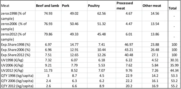
3.1.2 Descriptive statistics

Average zero consumption, expenditure shares, unit values and quantities are presented below (Table 2). As can be seen, there is very little change in zero consumption, apart from poultry, where zero observations dropped drastically from 1998 to 2012. Expenditure shares given to beef and lamb, poultry, and composite dishes have been rising since 1998, whereas the portion of the food budget allotted to pork and processed meat have decreased.

112101 Meat of bovine animals, boneless 1126S1 Grilled, smoked, cooked and cured pork 112102 Meat of bovine animals, with bone 1126S2 Grilled, cured, etc. poultry

112103 Seasoned beef, uncooked 112605 Other cured meat

112301 Fresh, chilled or frozen meat of sheep and goat

112606 Meat in aspic

112201 Meat of swine, boneless 112701 Meat preserves

112202 Pork chops 112702 Other preserved meat preparations

112203 Ham, uncooked 112703 Cabbage rolls

112204 Other meat of swine with bone 112704 Meat cabbage and meat potato casseroles, etc.

112205 Seasoned pork, uncooked 1127S1 Meat balls, ground beef patties

1127S2 Salads, ready-to-eat and frozen soups of meat 1124 Fresh, chilled or frozen poultry 1127S3 Blood pancakes, blood sausages, etc.

1127S4 Ready-to-eat meals of meat and other meat preparations

112501 Salami 112801 Meat of reindeer

1125S1 Other sausages, cold cuts 112802 Other meat and game

112504 Liver pâté and pastes 112803 Liver and kidneys

112505 Frankfurters 112804 Blood, tongue, bone, knuckle, etc.

112506 Ring sausages 112805 Minced meat

112507 Other cooking sausages 112806 Mixed meat for Karelian stew

112508 Sausages n.e.c. 112807 Meat n.e.c.

I Beef and lamb

II Pork

III Poultry

IV Processed meat

IV Processed meat continues

(19)

Table 2. Summary of Household Budget Survey data. Years 1998, 2006 and 2012 included

Overall, all unit values have increased. The only decrease in unit values can be observed in poultry from 1998 to 2006, but the poultry unit value reaches a new high in 2012, and displays an overall all increase (Figure 4). As unit values are defined as physical expenditure divided by quantity, the slight decrease in the unit value of poultry was likely caused by a tremendous growth in the quantity of poultry that was demanded, which, in turn, exceeded the growth of poultry expenditures. These unit values will be discussed more carefully in the section that follows.

Figure 4. Development of the unit values in HBS data

In 1998 households marked their expenditures to consumption daybooks, whereas, in 2006 and 2012, households sent in receipts as records of their consumption patterns

Meat Beef and lamb Pork Poultry Processed

meat Other meat Total

zeros1998 (% of sample) 74.93 49.02 62.56 4.67 14.56 -zeros2006 (% of sample) 76.93 50.46 51.32 4.47 13.54 -zeros2012 (% of sample) 79.86 49.33 45.48 6.01 13.86 -Exp.Share1998 (%) 6.97 14.77 7.41 46.97 23.88 100 Exp.Share2006 (%) 6.96 12.91 10.44 43.21 26.48 100 Exp.Share2012 (%) 7.51 12.65 12.26 40.48 27.1 100 UV1998 (€/kg) 7.32 6.07 6.18 6.22 4.52 30.31 UV2006 (€/kg) 9.21 7.79 5.53 7.62 5.84 35.99 UV2012 (€/kg) 11.73 8.52 7.07 9.76 7.26 44.34 QTY 1998 (kg/capita) 3 8.7 4.5 22.9 14.2 53.3 QTY 2006 (kg/capita) 2.4 6.3 6.2 22.2 16.1 53.2 QTY 2012 (kg/capita) 2.6 6.6 8.9 20.2 16.9 55.2 0 2 4 6 8 10 12 14 Beef and lamb

Pork Poultry Processed

meat

Other meat

€ /

kg

Development of the Unit Values

UV1998 (€/kg) UV2006 (€/kg) UV2012 (€/kg)

(20)

for the survey. As the reliability of the daybooks was impossible to check, the physical quantities observed in 1998 may differ greatly from those in 2006 and 2012. Most likely, the consumption daybooks led to higher recorded quantities of unprocessed carcass meat (ruminant meat, pork, poultry) being consumed than receipts. (Aalto and Peltoniemi, 2014.) These quantities are not included in the probit equations, but since unit value equations also contain quantity variables, the “biased” quantities of 1998 may also affect elasticities.

Figure 5 very clearly displays this phenomenon. According to FBS (Figure 1), neither the physical quantity of ruminant meat nor that of pork has decreased from 1998 to 2006, which is the case when quantities are calculated from HBS data. Despite the fact that the consumed quantity of poultry has also increased from 1998 to 2006 in HBS, one can assume that in reality the growth might have been even larger. It is worth noting that the magnitudes of quantities are different in FBS and HBS data. The Food Balance Sheets calculate the amount of food that is available for consumers after imports and exports. The storage and food stuffs used for animal feed are also observed, but the FBS does not reveal how much of that food actually ends up in the home of the consumer. Therefore, HBS data is more reliable, despite omitting the proportion of food waste and being based on non-credible consumption daybooks.

Figure 5. Development of physical quantities in HBS data.

0 5 10 15 20 25 Beef and lamb

Pork Poultry Processed

meat Other meat kg / ca p ita / ye ar

Physical quantities per capita in HBS data

Quantity1998 Quantity2006 Quantity2012

(21)

Demand system modelling contains many indices, estimators, approximations and other corrections that must be accounted for in various stages. In order to work properly, the data has to be prepared carefully, as it may contain misspecifications, such as observations where the total expenditure of meat is zero or negative, or observations where the expenditure is zero even if the physical quantity is positive. Therefore, the observations described above must be deleted from the data sets. As is usual with demand analysis, some observations may have negative adjusted prices, leading to their removal as well. In total, nearly 200 observations were dropped from each data set (4129, 3823, 3377 observations in years 1998, 2006 and 2012 respectively).

3.1.3 Socio-economic variables

One important objective of the thesis is to identify demographic variables that influence consumption. The literature has adopted certain group of socio-demographic variables that are considered significant when speaking demand analysis (Khaliukova, 2013). Naturally, the selection of relevant variables depends on data. In this paper we utilize the model used by Irz (2017),who chose to incorporate the following socio-demographic variables after careful consideration: age, education, household size, number of kids, socio-professional status, income, region and season.

The socio-economic variables will be utilized in three different stages. First they explain consumers` choice problem in the probit model (discussed in section 3.3), then they help with estimating unit values (section 3.2) and finally they are used to estimate consumption in the LA-AIDS model (Irz, 2017). However the explanatory variables used in estimation are not entirely same in all estimation stages but the issue will be discussed later on. There are a couple of ways to include socio-demographic characteristic to demand system. The most frequently used methods are demographic scaling and demographic translating and according to Pollak and Wales (1981), the scaling method leads higher log-likelihood values. In the thesis demographic translating is adopted as it preserves linearity of the LA-AIDS model (Heien and Wessells, 1990).

Table 3 provides short survey of socio-economic variables. Age needs no definition, nor does household size. Still, it is interesting to see that average age has been increasing whereas households have become smaller. Other variables and definitions

(22)

based on demand analysis of Irz (2017). Dummy variables, which can get values one or zero, are compared to their reference group and, as usual in econometric analysis, reference variables are not used in the estimation process. With dummies, the mean column in the table reveals probability that a respondent belongs to that particular group.

Education was divided into three categories. Reference category refers basic education, which contains primary and lower secondary education, second category is intermediate grade and last group consist of tertiary education. Number of kids under or equal to the age of 16 has been decreasing, which is totally understandable when looking development in household size. Socio-economics groups are lower clerical and workers (known as blue collars), entrepreneurs and upper clerical (known as white collars), pensioners and finally students, farmers, unemployed and others. Proportion of pensioners has increased in study period, whereas number of people in other socio-professional categories has remained steady. Income was divided into quartiles and then reported per consumption units. The consumption unit is calculated so that head of the household gets largest weighting coefficient, whereas other family members get smaller weight, which is further dependent on their age. The region characteristics were defined differently between 1998, 2006 and 2012, and therefore new universal definitions were formed for this study. The regions used in the study are Helsinki and southern Finland, western Finland, northern and eastern Finland and the reference group is Archipelago region. As one can see from the table, there are not many observations from that region but it does not cause problems with estimation or interpretation (Table 3). The seasonal variables divide calendar year approximately to quarters.

(23)

Table 3. Descriptive statistics of the socio-demographic variables used in analysis

3.2 Unit values as a price substitutes

HBS data do not contain information relating to prices; during the estimation process, this can be problematic. A quick look at the AIDS model will reveal that price information is an essential element of this process, so without that information, the information found using these prices must be obtained in another way. One alternative for finding this information would be to divide expenditures by physical quantities and use the obtained values as a substitute for the price variable. (Deaton, 1988.) There is, however a problem with this solution – the value obtained using this method and the market price value are not directly proportionate, as this value does not remove the uncontrolled variable of consumer preference. For example, using this solution, despite the fact that a higher-income household might consume less meat, their budget allocation for meat products might be equal to that of a lower-income household because they prefer to buy higher quality meat. Similarly, increases in meat prices may push a low-income household to consume larger quantities of minced meat while reducing their consumption of higher quality meats, all the while allowing them to maintain a fairly constant budget for meat expenditures. Taking these scenarios into consideration, it becomes clear that the situation imagined using this method as an

min max mean SD min max mean SD min max mean SD

Age 17 97 49 16 17 96 51 17.00 18 95 53 17.00

Education (ed1, Low)

Medium (ed2) 0 1 0.36 0.48 0 1 0.13 0.34 0 1 0.38 0.49

High (ed3) 0 1 0.27 0.44 0 1 0.19 0.40 0 1 0.39 0.49

HH size 1 18 2.6 1.4 1 19 2.5 1.40 1 12 2.4 1.30

kids16 0 1 0.32 0.47 0 1 0.29 0.45 0 1 0.26 0.44

Socio-profit (soscat1, Blue collar)

White collar (soscat2) 0 1 0.2 0.4 0 1 0.26 0.44 0 1 0.25 0.44

Pensioners (soscat3) 0 1 0.24 0.43 0 1 0.27 0.45 0 1 0.3 0.46

Other (soscat4) 0 1 0.13 0.34 0 1 0.09 0.29 0 1 0.09 0.29

Income (inc1, Quartile 1)

Quartile 2 (inc2) 0 1 0.25 0.43 0 1 0.25 0.43 0 1 0.25 0.43

Quartile 3 (inc3) 0 1 0.25 0.43 0 1 0.25 0.43 0 1 0.25 0.43

Quartile 4 (inc4) 0 1 0.25 0.43 0 1 0.25 0.43 0 1 0.25 0.43

Region (regdum4, Archipelago) Helsinki and southern Finland (regdum1)

0 1 0.42 0.49 0 1 0.44 0.50 0 1 0.47 0.50 Western Finland (regdum2) 0 1 0.27 0.44 0 1 0.26 0.44 0 1 0.25 0.43 Northern and eastern Finland

(regdum3)

0 1 0.29 0.45 0 1 0.26 0.44 0 1 0.24 0.43 Annual quarter (seasdum4)

seasdum1 0 1 0.26 0.44 0 1 0.26 0.44 0 1 0.27 0.44

seasdum2 0 1 0.22 0.42 0 1 0.22 0.41 0 1 0.22 0.42

seasdum3 0 1 0.22 0.42 0 1 0.23 0.42 0 1 0.23 0.42

(24)

alternative is incomplete and somewhat misleading. Additionally, Deaton (1988) states that both expenditure and quantity estimates are affected by measurement errors, and, consequently, any unit values obtained using this method are contaminated by those errors. Without accounting for those errors the estimations obtained are likely to be biased (Irz, 2017).

In order for the obtained value to be a viable replacement for the price value in demand estimates, the unit values must first be adjusted to dispel possible bias and complications such as those mentioned above. One solution to this issue that was suggested by Cox and Wohlgenant (1986) was the incorporation of dummy variables such as income, education and household size in the obtaining of and correcting of these values. Another suggestion from Majumder et al (2012) proposed the insertion of a regional variable. Yet another proposal from Aepli and Finger (2013) extended the correction model further still by incorporating a time variable. However, in spite of these adjustments, the unit values obtained from these calculations can still deliver biased results (Gibson, 2005). A more comprehensive analysis regarding the unit values is provided in the Appendix.

3.3 Zero consumption

One characteristic of data obtained from the HBS is its considerable proportion of zero values. The two-week survey period utilized in the survey may be shorter than the consumption cycle of a consumer, which could result in a household not consuming a certain food item at all. This infrequency of purchases is often reason for zero values. However, it is also a possibility that the zero consumption of a certain product reflects a true corner solution where the price of the product is too high and the consumer cannot afford it. Additionally, the “true” zeros may refer consumers that buy meat at no price. In other words, the expenditure allocated to beef liver might simply be zero because the household in question consists only of vegetarians, or beef liver might just be an otherwise undesirable commodity for that household at its current income level. (Gould, 1992.)

A data set with a significant amount of zero values is referred to as “censored”. Positive data are usually utilized in the estimation process; however, the zero values must be accounted for, as any estimate made without regard for those zero values would be biased and inconsistent (Amemiya, 1985; Smutná, 2016). Researchers have often

(25)

approached censored data simply by ignoring zero values (Aborisade et al., 2017; Shibia et al., 2017), but this raises the question: Is that sample still random? Tiberti and Tiberti (2015) attempted to resolve the zero observation problem by adding one to each value in the data set and transform them into logarithms. Unfortunately, by generating information that is inaccurate and changing observations to one, one is assuming that a person actually bought meat, which is not the case with “true” zero observations.

There are a couple of ways how to approach censored data. Due to the complex nature of the multiple equations model, many straightforward one-stage systems that utilize maximum likelihood are not usable (Coelho et al., 2010). Therefore Haines, Guilkey and Popkin (1988) suggested two-stage methods for approaching a censored demand system. The Heckman two-step procedure was utilized by Heien and Wessells (1990) and for the sake of its simplicity it has been a popular tool in demand analysis. The first stage examines the dichotomous choice of the consumer: whether to buy certain good or not. Next, this probit model is used to make probability estimates of consumption for every household and food item being examined. In the second step, the inverse Mills ratio is calculated and is then added to each equation in the LA-AIDS model.

Later, Shonkwiler and Yen (1999) detected that the technique used by Heien and Wessel was theoretically inconsistent and could not be incorporated into Monte Carlo simulations well (Coelho et al., 2010, 2010; Heien and Wessells, 1990). While the method proposed by Shonkwiler and Yen (henceforth SY) has received criticism (Tauchmann, 2005), it is the method that will be utilized in this study. Like the Heien and Wessel method, the SY method also consists of two steps. Once again, the first step examines the consumer decision of whether to purchase a specific meat product or not. As many variables influence this decision, various socio-demographic variables must be considered in explaining the choice of the consumer (Shonkwiler and Yen, 1999). In the second step, the probability density function (PDF) 𝜙 and the cumulative probability function (CDF) 𝛷 obtained from fitted values of probit equations are introduced to the LA-AIDS model.

(26)

4 Estimation procedure

According to Akbay et al. (2008) “Estimation of a censored demand system with household survey data is one of the most challenging tasks in applied econometrics”. The censored LA-AIDS model has to be estimated in two steps. First, the probit equations are used to determine whether a household consumes certain meat aggregate or not. The main outcomes of these equations are the cumulative distribution function (CDF) and the probability density function (PDF), which are used in the second step of the estimation process. In the second step, corrected unit values are also needed as substitutes for price variables. So, before the final estimation can be completed, both the probit equations and the unit value equations must be calculated separately. The LA-AIDS model, as presented below in equation (7), is in its final form, which will be used in this study:

(7) 𝑤_𝑖 = 𝛷𝑖ℎ∗ [𝛼𝑖+ ∑ 𝛾𝑖𝑗 𝑛 𝑗=1 𝑙𝑛𝑃𝑗+ 𝛽𝑖(ln 𝑋ℎ− ∑ 𝑤𝑖ln 𝑃𝑖) + ∑ λ𝑘𝐷𝑘ℎ 𝑘 𝑖 ] +𝜹𝑖𝜙𝑖ℎ+ 𝑢𝑖 4.1 LA-AIDS in R

There are a couple of ways to approach the equations used in the LA-AIDS model. Once the unit values have been corrected, the simplest approach is to use R package “micEconAids” as authored by Henningsen (2017a). In order to fully understand what is happening here, it is essential to understand the procedures that are taking place when using this package. Unfortunately the R package does not make estimation with censored data possible, and therefore all the formulas have to be formed manually if one wants to take zero-consumption into account.

Step 1 Probit and unit value equations

After defining the socio-demographic variables, the first-step independent probit equations can be regressed for every meat aggregate. Regression as used in this paper is based on Irz (2017), and the procedure is presented in detail in the Appendix. It is worth noting that price variables are not included in the probit equations as they would disrupt the homogeneity assumption. Instead, in the probit equations, only socio-demographic variables are included as explanatory variables (Bilgic and Yen, 2013). Additionally, the unit value equations are independent, and a separate regression can be run for each meat category “i”. As Cox and Wohlgenant (1986) proposed, the

(27)

quality-adjusted prices, or the final price substitutes, consist of the corrected average prices and residuals. The residuals are obtained simply by applying an OLS regression, where the dependent variable (unit value) is explained by household characteristics and the physical quantity the chosen category. Physical quantity is defined according to Capacci and Mazzocchi (2011), where the larger the quantity purchased is, the lower the unit value will be. Due to zero consumption, the average prices for non-consuming households must also be taken into account. In order to correct for region and season linked differences in prices, fitted values were applied in the unit value equations. Without regional and seasonal correction, the average price substitutes that were obtained would be biased. (Cox and Wohlgenant, 1986; Irz, 2017; Park and Capps Jr, 1997.) The estimation process and the R codes used in the study are presented in greater detail in the Appendix.

Step 2 The LA-AIDS model with Iterative Seemingly Unrelated Regression

As this study examined five aggregated meat groups, the number of equations used was also five. In the second step, these equations had to be estimated simultaneously due to cooperative actions between the aggregate groups. In R, this can be done with help of a “systemfit” package (Henningsen and Hamann, 2007). The system of equations can be estimated using the seemingly unrelated regression (SUR) model, the ordinary least squares (OLS) model, or the weighted least squares (WLS) model if the regressors are exogenous (as was assumed earlier). If the disturbance terms are correlated, the estimates of foregoing models are biased and the two-stage least squares (2SLS), weighted two-stage least squares (W2SLS), or three-stage least squares (3SLS) estimation models should be used instead. (Henningsen and Hamann, 2007.) When the number of iterations is larger than one, the SUR estimator is referred to as iterated seemingly unrelated regression (ITSUR or ISUR). Because ITSUR is well tested and frequently used in LA-AIDS estimation, it was utilized in this study. The SUR estimates are based on one-step covariances (obtained by OLS or 2SLS), whereas ITSUR calculates a new covariance matrix from previous estimations until the estimated coefficients converge. (Henningsen and Hamann, 2007.) Another frequently used estimator is the full information maximum likelihood (FIML) estimator, but according to Henningsen (2017b), ITSUR often converges to FIML.

(28)

As budget shares sum-up to one, the residual covariance matrix will be singular, which is problematic for estimations. As a result, one of the equations must be dropped from system; however, the missing coefficients can be obtained with the assistance of an adding-up restriction (Blanciforti and Green, 1983). However, after censoring, budget shares do not sum up to one anymore, making it possible to estimate all five equations simultaneously (Yen et al., 2002). Some studies actually recommend that estimations be calculated in this manner. Still, the majority of censored demand system studies drop one equation when estimating their model. This is because, according to Akbay et al. (2008), the results obtained using this method are typically similar despite the fact that the estimation was performed by omitting one equation.

This study utilized the method where one equation was dropped before running the system of equations in R. While an estimation using all five meat equations would have been possible, including the fifth equation led to coefficients that were very small, resulting in estimates that were uncomfortably close to minus unity or unity (depending on elasticities). Similarly, researchers utilizing all n equations in their estimations (Akbay et al., 2007; Yen et al., 2002) estimated only n-1equations in their later studies (Akbay et al., 2008; Bilgic and Yen, 2013). Because of this, it was decided that an estimation using only four meat aggregates would better suit this study. However, the selection of meat group that should be omitted is complicated, as the results are not quite invariant to the group selected (Bilgic and Yen, 2013; Boysen, 2016; Pudney, 1989).

Because there was no natural residual group, the beef and lamb group equation was dropped from the model. This group was dropped because it was heavily censored, which could have skewed the final results of the study. This decision was also based on a similar decision made by Yen and Lin (2006) who dropped the highly censored beef group from their study, as it would have affected the accuracy of the elasticities for the beef group obtained in their estimations. By comparing the results with beef and lamb omitted to models where some other meat was omitted, the expenditure elasticity of the beef and lamb group became higher. Coefficients of the LA-AIDS model are presented in the Appendix.

(29)

4.2 Testing linear restrictions.

The homogeneity and symmetry restrictions can be implemented beforehand and are easily testable. There are a few ways of testing the restrictions: the F test, Wald tests and the likelihood ratio (LR) test. The formulas of these tests were proposed by Henningsen and Hamann (2007) and in this thesis they are applied symbolically. The null hypothesis of the tests assumes homogeneity in expenditures and prices, which denotes that proportional changes in prices and expenditures have no effect on demand. So, this simply implies that the sum of the price parameters in all equations equals zero, as can be seen in (5).

Homogeneity can be implemented in every equation separately, which is not case with symmetry (Deaton and Muellbauer, 1980a). However, as the first equation is dropped from the system, homogeneity cannot be implemented for the beef and lamb category. The homogeneity restriction held in 2006 and 2012 as the likelihood ratio test was unable to reject the null hypothesis at a 95 % level of significance. In 1998 the homogeneity restriction held only for processed meat and other meat products. Both the symmetry restriction and symmetry with homogeneity were rejected (Table 4): Table 4. Testing the restrictions. LR test results

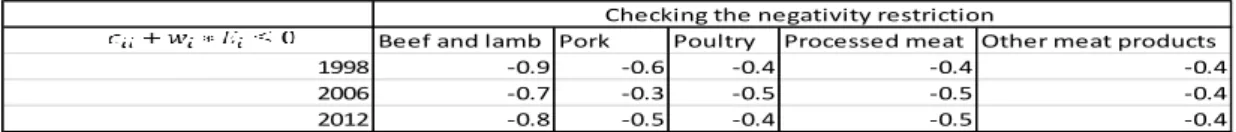
The fourth - and rarely observed - property is negativity. When the expenditure function is concave in relation to prices, the substitution matrix is negative semidefinite, and the diagonal elements of the matrix are negative as well. This restriction can be tested only afterwards by, for example, checking whether the sum of the Marshallian own-price elasticities and the expenditure elasticities of multiple budget shares of a certain group are less than or equal to zero (Edgerton et al., 1996). In this paper, the negativity restriction holds true (Table 5):

Table 5. Testing the negativity restriction (Edgerton et al., 1996)

1998 2006 2012

Homogeneity imposed Pr(>Chisq) 0.695 (eq4, eq5) 0.213 0.073

Symmetry imposed Pr(>Chisq) 0.0310 0.0039 0.0240

Homogeneity and symmetry imposed Pr(>Chisq) 0.0028 0.0074 0.0001

Beef and lamb Pork Poultry Processed meat Other meat products

1998 -0.9 -0.6 -0.4 -0.4 -0.4

2006 -0.7 -0.3 -0.5 -0.5 -0.4

2012 -0.8 -0.5 -0.4 -0.5 -0.4

(30)

4.3 Elasticities

Generally, the articles related to demand systems result in either Hicksian (compensated) or Marshallian (uncompensated) elasticities without exception. Own-price and expenditure elasticities are of particular interest. One could say that elasticities are the most important result of demand analyses, as the other coefficients and results of the AIDS model can be difficult to interpret. (Irz, 2017) Elasticities are determined using the parameter estimates found using the LA-AIDS model. Formulas of expenditure elasticities, Marshallian demand elasticities, and Hicksian demand elasticities are defined in the Appendix. In this analysis, elasticities have been calculated by using the unconditional means of the expenditure shares as proposed by Yen and Lin (2006).

Expenditure or income elasticity is defined as 𝑒_𝑖 =% 𝑐ℎ𝑎𝑛𝑔𝑒 𝑖𝑛 𝑑𝑒𝑚𝑎𝑛𝑑

% 𝑐ℎ𝑎𝑛𝑔𝑒 𝑖𝑛 𝑖𝑛𝑐𝑜𝑚𝑒. Therefore, the

elasticity reveals how much the quantity demanded changes as a result of a one per cent change in the total expenditure of meat products. In general expenditure elasticities divide goods to necessity, luxury or inferior goods. When the elasticity is larger than one, the good is luxury and changes in quantity demanded are larger than changes in expenditures. In the case that the elasticity is between zero and one, the good is known as a necessity. Together luxuries and necessities are known as normal goods, as quantity demanded rises when expenditure rises. Increasing expenditures can also lead to decreasing the quantity demanded when expenditure elasticity is negative and a good is inferior. (Varian, 2014.)

Cross-price elasticity reveals how much the demanded quantity of good “i” changes when price of good “j” changes by one per cent. In a case where the value of that elasticity is negative, goods “i” and “j” are complements, whereas a positive sign denotes substitution. Own-price elasticity measures the change in demand that occurs when a good’s own price changes. Due to restrictions and consumer theory, own-price elasticities are negative unless the good is a Giffen good, in which case rises in price would increase the demand. (Deaton and Muellbauer, 1980a; Edgerton et al., 1996.) Demand elasticities are often defined as elastic or inelastic depending on the magnitude of elasticity. If the elasticity is smaller than minus one, the demand is elastic whereas demand is inelastic when the elasticity is between minus one and zero (Varian, 2014). Hicksian elasticities measure how good or bad the price changes are for those consumers they effect. For example, if the price of a good rises but this change would

(31)

be compensated to the consumer, the question is how much would s/he buy? Thus, Hicksian elasticities give information relating to what happens to consumers’ demand due to price changes when holding utility constant. (Irz, 2017.)

Differences between Marshallian and Hicksian cross-price elasticities may be difficult to understand without adequate information regarding the substitution and income effects in general. Marshallian demand functions produce gross complements and substitutes, where gross denotes both the income and substitution effects. Consequently, Hicksian demand functions produce net complements (substitutes) when the effect of income is not present at all. Due to presence of the income effect, good “i” can be a gross substitute for good “j”, and at the same time “j” can be a cross complement to “i”. So, the gross definitions are not symmetric. Instead the net definitions are symmetric in sign. For example, if the price of the first meat group rises, and this has an effect on the consumption of the second group, the effect would be similar to the hypothetical price increasing in the second group that would affect the first group. Therefore, the price ratio is the only aspect that changes between those two goods when a price changes. (Varian, 2014.)

Meat elasticities obtained in different studies differ depending on county, culture, religion and income level. More so, the model used in an estimation analysis as well as the different specifications used can change elasticity values, and therefore the results may not be comparable. Gallet (2010) summarized the meat demand elasticities of different studies, and in general the price elasticity of poultry seemed to be the lowest whereas the elasticity of the beef and lamb category reached the highest values. However, sometimes the results are the opposite. Despite a median price elasticity of -0.77 from a sample of hundreds of studies, estimates varied greatly with a standard deviation of 1.28. According to Gallet (2010) price elasticity is strongly affected by the estimation method and specification of demand, whereas the location of demand and data characteristics have minor impact.

Literature provides a broad range of elasticity formulas, which differ greatly from one another. As with demand modelling, it is also preferable to use ready-made approximations and simplifications when calculating elasticities, so that the author does not need to derive elasticities from original expressions. While using ready-made approximations and simplifications accelerates the process, it also causes uncertainty

(32)

as the author knows neither where the elasticities come from nor which elasticities should be used. Expenditure elasticities are similar, but especially Marshallian elasticities with censored systems can cause problems. However, there are also clear mistakes with elasticity formulas. Many elasticity expressions are based on Green and Alston (1990), and while the elasticity formulas of the LA-AIDS model were determined to be incorrect later (Green and Alston, 1991), they are still present in some studies (Aborisade et al., 2017).

Yen and Lin (2006) suggested that in censored systems elasticities should be calculated using the unconditional means of the expenditure shares rather than sample means. In this study we utilize the derivations suggested by Bilgic and Yen (2013). The system used to calculate the means can greatly impact the final elasticities that are found. Values of the CDF can be computed for individuals and then averaged, or the CDF values can be calculated directly from the parameters of the corresponding exogenous variables. Derivations of the formulas are presented in the Appendix.

(33)

5 Results

5.1 Probit and unit value equations

The estimated coefficients from the first-stage probit equations aim at explaining a positive consumption by the consumer. The absolute value of the coefficients reveals to which degree the explanatory variables influence that choice. In other words, the coefficients identify the factors that increase or decrease the probability that a consumer will decide to buy a good belonging to a certain meat category. Thus, it is worth noting that these coefficients do not reveal how much consumption levels change due to household characteristics, but instead they reveal whether consumption becomes more or less probable. The significances of the factors have been marked with asterisks, and standard errors have been provided in parentheses. The coefficients of dummy variables (education, socio economic status, income, region and season) provide information pertaining to the probability effect in relation to the corresponding reference category, which has been excluded from the table. These determinants are presented for all three data sets used in the study. (Table 6.)

(34)

Table 6. Coefficients of estimated probit equations. (Significance levels *p<0.1; **p<0.05; ***p<0.01, standard errors in parentheses)

Apart from a few observations, age was consistently a significant factor. Even though the effect of aging is not great, it allows for the assumption that young people are less likely to buy meat products (apart from poultry) than their older counterparts. However, the literature does not take a stand on this hypothesis. While the effects of education on meat product purchases seem to be minimal, there is some evidence that

1998 2006 2012 1998 2006 2012 1998 2006 2012 1998 2006 2012 1998 2006 2012 age 0.01*** _0.003 _0.004* _0.01*** _0.01*** _0.01*** _{-0.002 -0.01}*** _-0.01** _0.01** _0.01** _0.02*** _0.002 _-0.01*** _0.003 -0.002 -0.002 -0.002 -0.002 -0.002 -0.002 -0.002 -0.002 -0.002 -0.003 -0 -0 -0.002 -0.002 -0.002 ed2 0.01 -0.05 0.01 -0.06 -0.004 0.02 0.07 0.16** _0.16** _-0.11 _-0.13 _0.05 _0.02 _-0.14* _0.1 -0.06 -0.07 -0.07 -0.05 -0.06 -0.06 -0.05 -0.06 -0.06 -0.09 -0.12 -0.1 -0.07 -0.08 -0.08 ed3 -0.06 0.05 0.03 -0.20*** _-0.20*** _-0.08 _0.18*** _0.07 _0.12* _-0.13 _-0.15 _0.01 _-0.06 _-0.20** _0.06 -0.06 -0.07 -0.07 -0.06 -0.06 -0.07 -0.06 -0.07 -0.07 -0.11 -0.12 -0.11 -0.07 -0.08 -0.08 HH size 0.17*** _0.11*** _0.09*** _0.17*** _0.23*** _0.15*** _0.11*** _0.15*** _0.25*** _0.20*** _0.31*** _0.24*** _0.29*** _0.25*** _0.29*** -0.02 -0.02 -0.03 -0.02 -0.03 -0.03 -0.02 -0.03 -0.03 -0.05 -0.06 -0.05 -0.04 -0.04 -0.04 kids<=16 -0.08 -0.06 0.11 -0.01 -0.23*** 0.003 0.12* 0.09 -0.01 -0.06 -0.08 -0.09 0.1 0.06 0.03 -0.07 -0.08 -0.09 -0.07 -0.07 -0.08 -0.07 -0.07 -0.08 -0.13 -0.15 -0.14 -0.09 -0.11 -0.11 soscat2 0.14** _-0.06 _0.06 _0.07 _-0.08 _-0.07 _0.02 _0.13** _0.06 _-0.07 _0.03 _-0.02 _-0.14* _-0.03 _-0.29*** -0.06 -0.07 -0.07 -0.06 -0.06 -0.06 -0.06 -0.06 -0.06 -0.11 -0.12 -0.11 -0.08 -0.08 -0.08 soscat3 0.002 0.01 0.03 -0.12 -0.12 -0.07 -0.12 -0.08 0.02 -0.23* _0.02 _-0.09 _-0.26*** _0.13 _-0.18* -0.08 -0.09 -0.09 -0.08 -0.08 -0.08 -0.08 -0.08 -0.08 -0.13 -0.14 -0.13 -0.09 -0.1 -0.1 soscat4 0.09 -0.03 0.12 -0.01 -0.15* _-0.07 _-0.1 _-0.09 _-0.01 _-0.34*** _-0.14 _-0.23* _-0.17** _-0.21** _-0.11 -0.08 -0.09 -0.1 -0.07 -0.08 -0.08 -0.07 -0.08 -0.09 -0.11 -0.13 -0.12 -0.09 -0.1 -0.11 inc2 0.18*** _0.09 _0.19** _0.14** _0.17*** _0.16** _0.19*** _0.16** _0.13* _0.04 _0.29*** _0.11 _0.01 _0.20*** _0.11 -0.07 -0.07 -0.08 -0.06 -0.06 -0.06 -0.06 -0.06 -0.06 -0.1 -0.11 -0.1 -0.07 -0.08 -0.08 inc3 0.22*** _0.23*** _0.19** _0.24*** _0.26*** _0.21*** _0.31*** _0.29*** _0.20*** _0.16 _0.42*** _0.15 _0.09 _0.30*** _0.26*** -0.07 -0.07 -0.08 -0.06 -0.06 -0.07 -0.06 -0.06 -0.07 -0.11 -0.12 -0.11 -0.08 -0.08 -0.09 inc4 0.39*** _0.42*** _0.48*** _0.22*** _0.26*** _0.14* _0.30*** _0.30*** _0.20*** _0.27** _0.45*** _0.17 _0.05 _0.24*** _0.22** -0.07 -0.08 -0.08 -0.07 -0.07 -0.07 -0.07 -0.07 -0.07 -0.12 -0.13 -0.12 -0.08 -0.09 -0.09 regdum1 -0.51*** _-0.37*** _-0.59*** _{-0.003 -0.09} _-0.33*** _0.39** _0.26** _0.13 _0.45* _0.35* _0.08 _-0.45* _0.39*** _-0.01 -0.17 -0.11 -0.12 -0.17 -0.11 -0.12 -0.18 -0.11 -0.12 -0.23 -0.18 -0.2 -0.26 -0.13 -0.15 regdum2 -0.58*** _-0.42*** _-0.59*** _0.13 _-0.18 _-0.29** _0.35* _0.31*** _0.17 _0.58** _0.39** _0.15 _-0.39 _0.50*** _0.11 -0.17 -0.12 -0.12 -0.17 -0.11 -0.12 -0.18 -0.12 -0.12 -0.24 -0.19 -0.2 -0.26 -0.13 -0.16 regdum3 -0.80*** _-0.48*** _-0.67*** _0.03 _-0.16 _-0.28** _0.34* _0.12 _0.14 _0.68*** _0.27 _0.17 _-0.34 _0.56*** _0.16 -0.17 -0.12 -0.12 -0.17 -0.11 -0.12 -0.18 -0.12 -0.12 -0.24 -0.19 -0.2 -0.27 -0.13 -0.16 seasdum1 0.09 0.15** _0.18*** _-0.05 _-0.07 _0.04 _0.09 _-0.12** _0.07 _0.15 _0.06 _-0.04 _-0.02 _0.04 _0.08 -0.06 -0.06 -0.07 -0.05 -0.06 -0.06 -0.05 -0.06 -0.06 -0.09 -0.1 -0.1 -0.07 -0.07 -0.08 seasdum2 0.10* _-0.08 _0.05 _0.03 _0.08 _0.24*** _0.004 _0.02 _-0.01 _0.17* _0.09 _0.03 _0.02 _-0.11 _-0.12 -0.06 -0.07 -0.07 -0.06 -0.06 -0.06 -0.06 -0.06 -0.06 -0.1 -0.11 -0.1 -0.07 -0.07 -0.08 seasdum3 0.02 0.03 -0.02 -0.04 0.04 0.03 0.15*** _0.10* _0.08 _0.19* _0.08 _0.02 _0.04 _-0.01 _-0.01 -0.06 -0.06 -0.07 -0.06 -0.06 -0.06 -0.06 -0.06 -0.06 -0.1 -0.1 -0.1 -0.07 -0.07 -0.08 Constant -1.28*** _-0.96*** _-1.03*** _-1.09*** _-0.92*** _-0.59*** _-1.20*** _-0.50*** _-0.62*** _0.33 _0.12 _0.01 _0.74** _0.36* _0.17 -0.22 -0.17 -0.19 -0.21 -0.16 -0.18 -0.22 -0.16 -0.18 -0.31 -0.25 -0.28 -0.3 -0.19 -0.22 Beef and lamb Pork Poultry Processed meat Other meat products