The Pricing of Options with Jump Diffusion and Stochastic Volatility

(1)

Faculty of Industrial Engineering, Mechanical Engineering and

Computer Science

Faculty of Industrial Engineering, Mechanical Engineering and

Computer Science

The Pricing of Options with Jump

Diffusion and Stochastic Volatility

(2)

(3)

THE PRICING OF OPTIONS WITH JUMP

DIFFUSION AND STOCHASTIC VOLATILITY

Linghao Yi

60 ECTS thesis submitted in partial fulfillment of a

Magister Scientiarum degree in Financial Engineering

Advisors

Olafur Petur Palsson

Birgir Hrafnkelsson

Faculty Representative

Eggert Throstur Thorarinsson

Faculty of Industrial Engineering, Mechanical Engineering and

Computer Science

School of Engineering and Natural Sciences

University of Iceland

(4)

The Pricing of Options with Jump Diffusion and Stochastic Volatility

60 ECTS thesis submitted in partial fulfillment of a M.Sc. degree in Financial Engineering Copyright c 2010 Linghao Yi

Faculty of Industrial Engineering, Mechanical Engineering and Computer Science

School of Engineering and Natural Sciences University of Iceland Hjardarhagi 2-6 107, Reykjavik, Reykjavik Iceland Telephone: 525 4000 Bibliographic information:

Linghao Yi, 2010, The Pricing of Options with Jump Diffusion and Stochastic Volatility, M.Sc. thesis, Faculty of Industrial Engineering, Mechanical Engineering and

Computer Science, University of Iceland.

ISBN XX

Printing: Háskólaprent, Fálkagata 2, 107 Reykjavik Reykjavik, Iceland, July 2010

(5)

(6)

(7)

Abstract

The Black-Scholes model has been widely used in option pricing for roughly four decades. However, there are two puzzles that have turned out to be difficult to explain with the Black-Scholes model: the leptokurtic feature and the volatility smile. In this study, the two puzzles will be investigated. An improved model – a double exponential jump diffusion model (referred to as the Kou model) will be introduced. The Monte Carlo method will be used to simulate the Black-Scholes model and the double exponential jump diffusion model to price the IBM call option. The call option prices estimated by both models will be compared to the market call prices. The results show that the call option prices estimated by the double exponential jump diffusion model fit the IBM market call option prices better than the call option prices estimated by the Black-Scholes model do.

The volatility in both the Black-Scholes model and the double exponential jump diffusion model is assumed to be a constant. However, it is stochastic in reality. Two new models based on the Black-Scholes model and the double exponential jump diffusion model with a stochastic volatility will be developed. The stochastic volatility is determined by a GARCH(1,1) model. The advantage of GARCH model is that GARCH model captures some features associated with financial time series,

(8)

both the new models will be presented. Then the Monte Carlo simulation will be applied to the two new models to price the IBM call option. Finally, the call option prices estimated by the four models will be compared to the market call option prices. The performance of the four models will be evaluated by statistical methods such as mean absolute error (MAE), mean square error (MSE), root mean square error (RMSE), normalized root mean square error (NRMSE), and information ratio (IR). The results show that the double exponential jump diffusion model performs the best for the lower strike prices and the Kou & GARCH model has the best performance for the higher strike prices. Theoretically, the Kou & GARCH model is expected to be the best model among the four models. Some possible reasons and suggestions will be given in the discussion.

(9)

Preface

It was good to study Financial Engineering in Faculty of Industrial Engineering, Mechanical Engineering and Computer Science at the University of Iceland.

First, I am thankful to my advisor, professor Olafur Petur Palsson, for his advice, comments and corrections on my thesis. He introduced to me two good tools, time series analysis and technical analysis. In the summer of 2008, I worked on the "Currency Exchange Trading Strategy Analysis" under his supervision.

I also give my thanks to my second advisor, research professor Birgir Hrafnkelsson, for his advice, in particular, for his comments and corrections on statistics.

I spent one year at the University of California at Berkeley in the school year of 2008 – 2009 as a visiting research student where I took several financial engineering and economics courses. I got expertise guidance and help from professor Xin Guo, professor Ilan Adler, professor J. G. Shanthikumar, as well as help from professor Philip M. Kaminsky and staff Mike Campbell. I am grateful to these great people. Finally, I would like to give my thanks to my husband, professor Jon Tomas Gud-mundsson, for his encouragement, support and help.

(10)

Linghao Yi

Faculty of Industrial Engineering, Mechanical Engineering and Computer Science

University of Iceland Reykjavik, Iceland July 2010

(11)

Nomenclature

α the GARCH error coefficient

β the GARCH lag coefficient

B a Bernoulli random variable

c call option price

d dividend rate

dq a Poisson counter

∆t time period

δ standard deviation of the logarithm of the jump size distribution

E the expectation value

ηu means of positive jump

ηd means of negative jump

J jump size

K strike price

κ a mean-reverting rate

λ jump intensity

µ drift, mean of daily log return, mean of normal distribution

ν mean of the logarithm of the jump size distribution

(16)

P physical probability Q risk-neutral probability

ω a constant for GARCH(1,1)

φ normal distribution process

p put option price

p probability of upward jump

q probability of downward jump

ρ correlation coefficient

r daily log return

Rt daily simple return

rt daily log return

rf riskfree interest rate

S asset price, underlying price, stock price

S0 an initial stock price

S(t) asset price, underlying price, stock price in continuous time

St asset price, underlying price, stock price in discrete time

σ volatility, standard deviation of daily log return

T time to maturity t time τ time period θ a log-term variance ε a volatility of volatility V the variance

V(t) the diffusion component of return variance

W(t) a standard Wiener process in continuous time

(17)

Ws₍_t₎ _{a standard Wiener process, used to describe} _S₍_t₎

Wv₍_t₎ _{a standard Wiener process, used to describe} _V₍_t₎

Wλ₍_t₎_{a standard Wiener process, used to describe} _λ₍_t₎

ξ+ an exponential random variable with probabilityp upward

ξ₋ an exponential random variable with probabilityq downward

(18)

(19)

1 Introduction

1.1 Background

The Black-Scholes model (Black and Scholes, 1973), which is based on Brownian motion and normal distribution, has been widely used to model the return of assets and to price financial option for almost four decades. However, many empirical evidences have recently shown two puzzles, namely the leptokurtic feature that the return distribution of assets may have a higher peak and two asymmetric heavy tails than those of normal distribution, as well as an abnormality, often referred to as ’volatility smile’, that is observed in option pricing (Kou, 2002; Kou and Wang, 2003, 2004).

Before these empirical puzzles are explored, a few fundamental concepts and models that this study is based on will be introduced.

1.1.1 Asset returns

(20)

1 Introduction

simple gross return when holding an asset for one period from date t₋1 to date t

is given as (Tsay, 2005)

1 +Rt=

St

St−1

The corresponding one-period simple net return (often referred to as simple return) is Rt= St St−1 − 1 = St−St−1 St−1

and the multiperiod simple gross return when holding the asset forkperiods between date t₋k to datet is given as

1 +Rt[k] = St St−k = St St−1 × St−1 St−2 × · · · × St−k+1 St−k = (1 +Rt)(1 +Rt−1)· · ·(1 +Rt−k+1) = k−1 Y j=0 (1 +Rt−j)

The log return is the natural logarithm of the simple gross return of an asset. Thus the one-period log return is

rt = log(1 +Rt) = log St St−1 = log (St)−log (St−1)

and the multiperiod log return is

rt[k] = log(1 +Rt[k]) = log [(1 +Rt)(1 +Rt−1)· · ·(Rt−k+1)]

= log(1 +Rt) + log(1 +Rt−1) +· · ·+ log(1 +Rt−k+1)

=rt+rt−1+· · ·+rt−k+1

Most of the time, log return will be used in this study. The advantages of the log return over the simple return are that the multiperiod log return is simply the sum

(21)

1.1 Background

of the one-period returns involved and the statistical properties of log returns are more tractable.

1.1.2 Geometric Brownian motion

Geometric Browian motion (GBM) is the simplest and probably the most popular specification in financial models. The Black-Scholes option pricing model assumes that the underlying state variable follows GBM. GBM specifies that the instanta-neous percentage change of the underlying asset has a constant driftµand volatility

σ (Baz and Chacko, 2004; Craine et al., 2000; Merton, 1971). It can be described by a stochastic differential equation

dS

S =µdt+σdWt (1.1)

where dWt is a Wiener process with a mean of zero and a variance equal to dt.

Equation (1.1) is known as the Black-Scholes equation (Derman and Kani, 1994a).

1.1.3 Black-Scholes option pricing model and return

Recall the Black-Scholes equation,

dS=µSdt+σSdWt (1.2)

then applying Ito’s Lemma, the following equation is obtained (Baz and Chacko, 2004). d[logS] = µ₋ σ 2 2 dt+σdWt (1.3)

(22)

1 Introduction

Now, suppose that asset prices are observed at discrete timesti, i.e. S(ti) =Si, with

∆t =ti+1−ti, then the following equation can be derived from equation (1.3).

logSi+1−logSi = log

Si+1 Si ≅ µ₋σ 2 2 ∆t+σφ√∆t (1.4)

whereφ follows a standard normal distribution. Now, if ∆t is sufficient small, then

∆t is much smaller than √∆t, so that equation (1.4) can be approximated by

log Si+1 Si = log Si+1 −Si+Si Si = log 1 + Si+1−Si Si ≅σφ√∆t (1.5)

Lets define the return Ri in the periodti+1−ti as

Ri =

Si+1−Si

Si

(1.6) then equation (1.5) becomes

log(1 +Ri)≅Ri =σφ

√

∆t (1.7)

Equation (1.7) shows that the return of asset S should be normally distributed (Forsyth, 2008). This study is based on this conclusion.

(23)

1.2 Learning from the data

1.2 Learning from the data

S&P 500 index historical data from January 1950 to June 2010 and IBM histori-cal stock prices from January 1962 to June 2010, as well as IBM option price on June 10, 2010 are used in this study. The data is downloaded from Yahoo finance (http://finance.yahoo.com).

The S&P 500 index daily log return from January 1950 to June 2010 is shown in Figure 1.1. From this figure, it can be noted that the largest spikes occurred around October 1987 due to the 1987 stock market crash. The biggest negative return appeared on October 19, 1987. The range of the daily log return during this period was from -21.155 to 7.997. The second largest spikes occurred in October 2008 at the beginning of the global financial crisis. It can also be observed that significant fluctuations occurred during the period 2000–2002, which are due to the internet bubble burst and the September 11 attacks. From the data shown in Figure 1.1, it is obvious that the stock market became significantly more volatile after 1985 than it was the preceding 35 years. Therefore, the focus in further study will be on the S&P 500 index value from 1985 to 2010.

The S&P 500 index from January 1985 to June 2010 on a linear scale and a log scale are shown in Figures 1.2 (a) and (b), respectively. From both figures, it can be noted that the tendency of the index value is upward before the year 2000, but the index value has become more volatile during the past decade. The stock crash in 1987 can also be observed, it appears to be a relatively small downward jump. Why is it different from what are observed in Figure 1.1? The reason is that the S&P index value is not so high in 1987 and it caused a huge negative return even though the price did not fall as much as today.

(24)

1 Introduction

Jan50 Jan60 Jan70 Jan80 Jan90 Jan00 Jan10

−25

−20

−15

−10

−5

0

5

10

15

20 time

S&P 500 daily log return[%]

Figure 1.1: The S&P 500 index daily log return from January 1950 to June 2010. The biggest negative spikes occurred on October 19, 1987 when the stock market crashed. The second biggest spikes occurred due to the "Panic of 2008". The spikes around 2000–2002 are due to the internet bubble burst and the September 11 attacks.

(25)

Jan85

Jan90

Jan95

Jan00

Jan05

Jan10

0

200

400

600

800 1000

1200

1400

1600

time

S&P 500 index value

(a)

Jan85

Jan90

Jan95

Jan00

Jan05

Jan10

5

5.5

6

6.5

7

7.5 time

S&P 500 index log scale

(b)

Figure 1.2: The S&P 500 index value from January 1985 to June 2010. (a) on a linear scale and (b) on a log scale. The tendency of index value is upward before the year 2000, However, it has become very volatile in the past decade. The 1987 stock market crash can be clearly observed.

(26)

1 Introduction

Jan00

Jan02

Jan04

Jan06

Jan08

Jan10

600

800 1000

1200

1400

1600

time

S&P 500 index value

Figure 1.3: The S&P 500 index value from January 2000 to June 2010 on a linear scale. The stock market has been very volatile during this decade.

In order to explore further the increasingly volatile period of the past decade, the S&P 500 index from January 2000 to June 2010 is shown in Figure 1.3. The value has fluctuated around the index value of about 1200 in the recent ten years and the upward tendency has disappeared. A big drop in the index value occurred after September 11, 2001 and the index value plummeted again around the global financial crisis in October 2008.

The distribution of the S&P 500 index daily log return is plotted in Figure 1.4. It is not normally distributed. The peak is significantly higher and the tails are fatter than a normal distribution would predict. This is the leptokurtic feature, which will be discussed in section 2.1.1. In the next chapter, the S&P data from 1950 to 2010 will be divided into two data sets in order to investigate whether there exists a difference in the distribution for different periods.

(27)

−4

0 −2

0

2

4

0.1

0.2

0.3

0.4

0.5

0.6

0.7 S&P 500 daily log return [%]

Probability density

SP500

Normal

Figure 1.4: Distribution of S&P 500 index daily log return from January 1950 to June 2010. It is clear that the daily log return is not normally distributed. The peak is higher and the tails are fatter than a normal distribution would predict.

(28)

1 Introduction

1.3 Structure of the thesis

This thesis is organized as follows: In this chapter, some basic concepts and models and assumptions are introduced. In Chapter 2, the two puzzles of the Black-Scholes model, which are not supported by the empirical phenomena, will be substantiated by real data. In Chapter 3, some modifications to the Black-Scholes model will be summarized; their advantages and disadvantages will be discussed, evaluated and compared. In Chapter 4, the double exponential jump-diffusion model (also referred to as the Kou model), will be discussed in more detail. In Chapter 5, the implementation and the algorithms simulating the Black-Scholes model and the Kou model will be given. Do they fit the real data? What are their errors? Which one is the better model? In Chapter 6, a stochastic volatility model based on GARCH will be developed. In Chapter 7, two new models based on the Black-Scholes model and the Kou model, respectively, but with stochastic volatility, will be introduced. These two new models are compared with the Black-Sholes model and the Kou model visually and statistically. Finally, the conclusion, limitation and future work is discussed in Chapter 8.

(29)

2 Problem Description

In this chapter, the two puzzles (often referred to as the two phenomena) not sup-ported by the Black-Scholes model in empirical studies will be demonstrated using real market data. Furthermore, the reasons for the two puzzles will be analyzed.

2.1 The two puzzles

Many empirical studies show two phenomena, the asymmetric leptokurtic features and the volatility smile, which are not accounted for by the Black-Sholes model (Kou, 2002; Maekawa et al., 2008). The leptokurtic feature emerged in Section 1.2. In the coming sections, the real market data and individual stock price data will be applied to explore the existence of the two phenomena.

2.1.1 Leptokurtic distributions

The asymmetric leptokurtic features – the return distribution is skewed to the one side (left side or right side) and has a higher peak and two heavier tails than those of normal distribution – are commonly observed empirically.

(30)

2 Problem Description

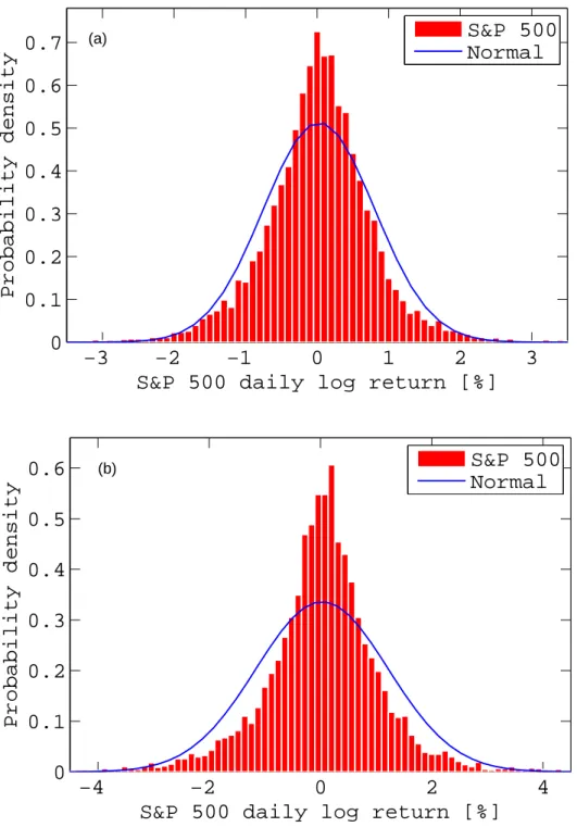
The purpose of this section is to check whether the leptokurtic phenomena exists on different data sets. First, the market data (S&P 500 index) is divided into two parts, one data set is for the period from January 1950 to December 1984, and the other data set is for the period from January 1985 to June 2010. The distribution of S&P 500 daily log return from 1950 to 1985 is shown in Figure 2.1(a). This daily log return does not follow a normal distribution because the peak is higher than a normal distribution would predict. Figure 2.1(b) shows the distribution of the S&P 500 index daily log return from January 1985 to June 2010. The leptokurtic feature can be noted in Figure 2.1(b). The peak is significantly higher than that of normal distribution. The skewness can be estimated by (Kou, 2008; Thomas, 2005).

ˆ S= 1 (n₋1)ˆσ3 n X i=1 (Xi−X¯)3 (2.1)

and the kurtosis is given as

ˆ K = 1 (n₋1)ˆσ4 n X i=1 (Xi−X¯)4 (2.2)

For the time period from 1950 to 1984, the kurtosis of S&P 500 is about 7.27, and the skewness is about -0.08. For the time period from 1985 to 2010, the kurtosis of S&P 500 is about 32.71, and the skewness is about -1.36. The negative skewness means that the return has a heavier left tail than the right tail. Or, the distribution is skewed to left side. So, the kurtosis is indeed significantly higher and the left tail is heavier than right tail for the period from 1985 to 2010.

An individual stock is also taken as an example, the data set is IBM historical stock price data from January 1962 to June 2010. The data set is split into two parts, one is for the period from January 1962 to December 1984, the other is for the period from January 1985 to June 2010. Their distributions of the daily log

(31)

2.1 The two puzzles

−3

−2

−1

0

1

2

3

0

0.1

0.2

0.3

0.4

0.5

0.6

0.7 S&P 500 daily log return [%]

Probability density

(a)

S&P 500

Normal

−4

−2

0

2

4

0

0.1

0.2

0.3

0.4

0.5

0.6 S&P 500 daily log return [%]

Probability density

(b)

S&P 500

Normal

Figure 2.1: (a) Distribution of the S&P 500 index daily log return from January 2, 1950 to December 31, 1984. (b) Distribution of the S&P 500 index daily log return from January 2, 1985 to June 10, 2010. Neither distributions is normally distributed; rather they are skewed to left side and have a higher peak and fatter tails compared to a normal distribution.

(32)

return are shown on Figures 2.2 (a) and (b). It is noted that neither is normally distributed but the IBM daily log return for the period from 1962 to 1984 fits a normal distribution somewhat better than the IBM daily log return for the period from 1985 to 2010. Both distributions have a high peak and two fatter tails than those of normal distribution. But the distribution from 1985 to 2010 has a heavier high peak. In other words, it is much more distributed around zero return. For the time period from 1962 to 1984, the kurtosis of IBM is about 6.32, and the skewness is about 0.24. For the time period from 1985 to 2010, the kurtosis of IBM is about 16.5, and the skewness is about -0.46. The kurtosis is significantly higher for the latter period. Also the distribution is slightly skewed to right side for the earlier period but to the left side for the later period.

As discussed in Section 1.1, the daily return distribution, according to the Black-Scholes model, is expected to be a normal distribution (Hull, 2005). However, the distribution of S&P 500 daily log return as seen in Figures 2.1 (a) and (b), and the distribution of IBM stock daily log return as seen in Figures 2.2 (a) and (b) do not follow a normal distribution. A normal distribution is also shown for comparison in all these figures withµandσ equal to the ML estimates. Note that the distribution for real data has a higher peak and fatter tails than those of the normal distribution. This means that there is a higher probability of zero return, and a large gain or loss compared to a normal distribution. Furthermore, as ∆t_→ 0, Geometric Brownian motion (Equation (1.1)) assumes that the probability of a large return also tends to zero. The amplitude of the return is proportional to √∆t, so that the tails of the distribution become unimportant. But, some large returns in small time increments can be seen in Figures 2.2 (a) and (b). It therefore appears that the Block-Scholes model is missing some important features.

(33)

−5

0

5

0

0.1

0.2

0.3

0.4

0.5

0.6

0.7 IBM daily log return [%]

Probability density

(a)

IBM

Normal

−6

−4

−2

0

2

4

6

0

0.05

0.1

0.15

0.2

0.25

0.3

0.35 IBM daily log return [%]

Probability density

(b)

IBM

Normal

Figure 2.2: (a) Distribution of IBM daily log return from January 2, 1962 to De-cember 31, 1984. (b) Distribution of IBM daily log return from January 2, 1985 to June 10, 2010. Neither distributions is normally distributed; they have a high peak and two fatter tails than those of normal distribution; but the high peak in (b) is heavier.

(34)

The leptokurtic features can also be proved by a quantile-quantile plot (Q-Q plot). The same data sets are used. A Q-Q plot of the S&P 500 index for the period from January 1985 to June 2010 is shown in Figure 2.3 (a), and a Q-Q plot of the IBM stock price for the period January 1985 to June 2010 is shown in Figure 2.3 (b). For a normal distribution, the plot should show a linear variation. However, as seen in Figures 2.3 (a) and (b), there is clearly a deviation from linear behavior.

The third proof of the feature is achieved by applying the Kolmogorov-Smirnov test (often referred to as KS-test) (Allen, 1978). By the Kolmogorov-Smirnov test, the values in the data vectorx are compared to a standard normal distribution.

The null hypothesis is H0 and the alternative hypothesis is H1, where

      

H0 : xhas a standard normal distribution,

H1 : xdoes not have a standard normal distribution.

(2.3)

if the test statistic of the KS-test is greater than the corresponding critical value, the null hypothesis, H0, is rejected at the 5% significance level; otherwise, the null

hypothesis, H0, is not rejected (Massey, 1951; Miller, 1956).

Lets define

x= r−µ

σ (2.4)

whereris daily log return,µis the mean of daily log return,σis a standard deviation of daily log return.

Based on a KS-test on the S&P 500 daily log return and the IBM stock daily log return, respectively, the null hypothesis is rejected in both cases. Therefore, it can be concluded that neither the daily log return of S&P 500 nor the daily log return

(35)

−4

−2

0

2

4 −20

−15

−10

−5

0

5

10

15

20 Standard Normal Quantiles

Quantiles of Input Sample

S&P 500 daily log return verus stanard normal

(a)

−4

−2

0

2

4 −20

−15

−10

−5

0

5

10

15

20 Standard Normal Quantiles

Quantiles of Input Sample

IBM stock daily log return verus stanard normal

(b)

Figure 2.3: (a) A Q-Q plot of the S&P 500 daily log return from January 2, 1985 to June 10, 2010. (b) A Q-Q plot of the IBM stock daily log return from January 2, 1985 to June 10, 2010. If the distribution of daily return is normal, the plot should be close to linear. It is clear that neither plots is linear, therefore, they are not normally distributed.

(36)

of IBM stock are normally distributed.

2.1.2 The volatility smile

If the Black-Scholes model is correct, then the implied volatility should be constant. That is, the observed implied volatility curve should look flat (Kou and Wang, 2004). But, in reality, the implied volatility curve often looks like a smile or a smirk. A plot of the implied volatility of an option versus its strike price is known as a volatility smile when the plotted curve looks like a human smile (Derman, 2003; Hull, 2005). Take the IBM call option as an example. For a 7-days maturity time, the IBM call option price versus the strike price is shown in Figure 2.4(a); the IBM implied volatility versus the strike price is shown in Figure 2.4(b), in which the "IBM volatil-ity smile" is observed. For a 92-days maturvolatil-ity time, Figure 2.5(a) shows the IBM call option price versus the strike price and Figure 2.5(b) shows the IBM implied volatility versus the strike price, including the "IBM volatility smile". When the IBM implied volatility versus the strike price is plotted for 162-days and 422-days, the curve of the implied volatility looks more like a "volatility skew" than a "volatil-ity smile", which are demonstrated in Appendix A.2 and A.3. That is, when the maturity time increase, the implied volatility monotonically decreases as the strike price increases (Hull, 2005).

The evolution of a "volatility smile" to a "volatility skew" with increasing maturity time is explored further in Figure 2.6. The x-axis is the time to maturity, the

y-axis is the strike price, the z-axis is the implied volatility. A "volatility smile" for a short time to maturity can clearly be observed; as the time to maturity is increased the curve becomes more flat. For multiple maturitiesT and multiple strike

(37)

100

110

120

130

140

150 −10

−5

0

5

10

15

20

25

30 Strike Price [USD]

Call Option Price [USD]

(a)

100

110

120

130

140

150

0.5

1

1.5

2

2.5

3

3.5

4

4.5

5

5.5 Strike Price [USD]

Implied Volatility [%]

(b)

Figure 2.4: (a) The call option price versus the strike price for IBM stock. (b) The observed implied volatility curve. The implied volatility versus the strike price of IBM just looks like a human smile; it is called the "IBM Volatility smile". The date of the analysis is June 10, 2010; the expiration date is June 18, 2010; the time to maturity T is 7 days; the initial IBM stock price, S0 is USD 123.9.

(38)

80

100

120

140

160

180 −10

0

10

20

30

40 Strike Price [USD]

Call Option Price [USD]

(a)

80

100

120

140

160

180

1.2

1.4

1.6

1.8

2

2.2

2.4

2.6

2.8 Strike Price [USD]

Implied Volatility [%]

(b)

Figure 2.5: (a) The call option price versus the strike price for IBM stock. The observed implied volatility curve. The implied volatility versus the strike price of IBM just looks like a human smile; it is called the "IBM Volatility smile". The date of the analysis is June 10, 2010; the expiration date is October 15, 2010; the time to maturityT is 92 days; the initial IBM stock price, S0 is USD 123.9.

(39)

0

200

400

100

120

140

160

0

1

2

3

4

5 T[day]

K[USD]

Volatility[%]

1.5

2

2.5

3

3.5

4

4.5

Figure 2.6: The observed 3-D IBM implied volatility with multiple maturitiesT and multiple strike prices K. It can be noted that the implied volatility plane is not flat and the implied volatility looks like a smile for shorter time to maturity T, but it becomes monotonously decreasing with increasing strike prices for longer time to maturity T.

prices K, when facing to the y-z plane (that is, the strike price - implied volatility plane), one notices that the curve looks more like a ’smile’ as the maturity time is shorter, but the curve is more like a ’smirk’ as the maturity time becomes longer. This phenomena is also discussed by Hull (2005) and by Andersen and Andersen (2000). One explanation for the smile in equity option concerns leverage. As a company’s equity declines in value, the company’s leverage increases. This means that the equity becomes more risky and its volatility increases. As a company’s equity increase in value, leverage decreases. Then the equity becomes less risky and its volatility decreases (Hull, 2005).

(40)

2.2 What is the reason ?

From the observation of the two phenomena, it can be concluded that the Black-Scholes model is not completely correct in describing neither the market behavior such as S&P 500 nor the behavior of individual stock price such as IBM. What is missing in the Black-Scholes model ?

The first problem is that the Black-Scholes model ignores the jump part in the process of asset pricing caused by overreaction or underreaction due to good and/or bad news coming from the market and/or from an individual company. In other words, the Black-Scholes model is completely correct in an ideal situation without outside world information. Thus, an extra jump part must be added to the Black-Scholes model in order to give a response to the underreaction (attributed to the high peak) and the overreaction (attributed to the heavy tails) to outside news (Kou, 2002, 2008).

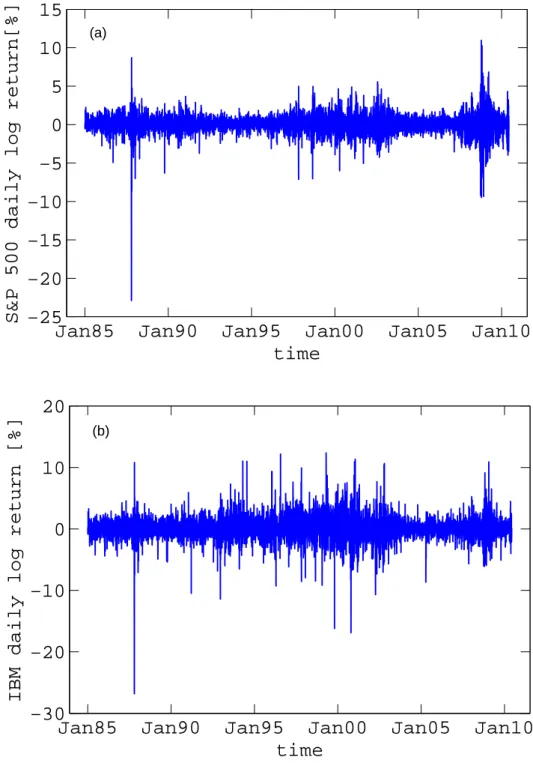
The time series plots of market data (S&P 500 index) and individual stock data (IBM) capture those jumps from good news or bad news, as seen in Figures 2.7 and 2.8. Figure 2.7 shows the temporal variation of the S&P 500 index from January 2005 to June 2010. There are indeed upward and downward jumps observed in the stock market such as the S&P 500 index; a big downward jump occurred around the global financial crisis in October 2008. Figure 2.8 shows the evolution of the IBM stock price from January 2005 to June 2010. The similar upward and downward jumps in the IBM stock price can be noticed, and the similar downward jump occurred around the global financial crisis time in October 2008.

These upward or downward jumps are also reflected in the daily log return time series plot, Figures 2.9 (a) and (b). Figure 2.9 (a) shows some upwards jumps (positive

(41)

2.2 What is the reason ?

Jan05

Jan06

Jan07

Jan08

Jan09

Jan10

600

800 1000

1200

1400

1600

time

S&P 500 index value

The big downward jump is related to the financial crisis in Oct. 2008.

The stock market crashed.

The upward jumps are related to good news.

Figure 2.7: The time series of S&P 500 index value in January 2005 - June 2010. It can be observed that there are some upward and downward jumps in the market price during these years. In October 2008, there is a large downward jump indicating the stock market crash due to the global financial crisis.

(42)

Jan05

Jan06

Jan07

Jan08

Jan09

Jan10

60

70

80

90

100

110

120

130

140 time

IBM stock price [USD]

The big downward jump is related to the financial crisis in Oct. 2008. The upward jumps are related to good news from market or company.

Figure 2.8: The time series of IBM stock price in January 2005 - June 2010. It can be observed that there are some upward and downward jumps in the IBM stock price during these years. In October 2008, there is a large jump downwards indicating that IBM stock was effected by the "Panic of 2008" due to the global financial crisis.

(43)

2.2 What is the reason ?

return) and some downwards jumps (negative return) in S&P 500 index value from 1985 to 2010. The biggest negative return is reflected in a large downward jump in the index value that is due to the stock market crash in October 1987. The spikes around October 2008 are related to the global financial crisis. Those upward and downward jumps were caused by the overreaction of investors. Figure 2.9 (b) shows some upwards jumps (positive return) and some downwards jumps (negative return) in IBM stock price from 1985 to 2010. The biggest spike is a huge downward jump in IBM stock price caused by the stock market crash in October 1987. There are a lot of spikes around 2000–2002; these spikes are upward and downward jumps in stock price related to the internet bubble bursts and the September 11 attacks. The same jumps are apparent in the IBM stock price as in the S&P 500 index value around the global financial crisis in October 2008. Throughout the period there are countless smaller spikes both upwards and downwards that are due to news from market and/or from individual companies. These jumps are ignored by the Black-Scholes model.

The second issue is that the volatility is assumed to be a constant in the Black-Scholes model, but it is stochastic in real life (Andersen and Andersen, 2000; An-dersen and Brotherton-Ratcliffe, 1998; AnAn-dersen et al., 2002; Derman and Kani, 1994a,b; Dupire, 1994; Heston, 1993; Stein and Stein, 1991). Figures 2.4 (b), 2.5 (b) and 2.6 demonstrate how the implied volatility changes as the time to maturity and the strike prices increases. Therefore, it is necessary to improve the Black-Scholes model in order to capture the two empirical phenomena mentioned above (Kou, 2002; Maekawa et al., 2008, 2005).

(44)

Jan85

Jan90

Jan95

Jan00

Jan05

Jan10

−25

−20

−15

−10

−5

0

5

10

15 time

S&P 500 daily log return[%]

(a)

Jan85

Jan90

Jan95

Jan00

Jan05

Jan10

−30

−20

−10

0

10

20 time

IBM daily log return [%]

(b)

Figure 2.9: (a) The time series of the S&P 500 index daily log return. (b) The time series of the IBM stock daily log return. The spike around October 1987 indicates a large negative return. This is the biggest stock market crash in history. IBM stock is also affected by the crash. The spikes around 2001 are related to the internet bubble burst and the September 11 attacks. There are many downwards and upwards jumps around 2000 to 2002 according to bad news or good news. The spikes around October 2008 are caused by the global financial crisis.

(45)

3 Overview of the Models

Many studies have been conducted to modify the Black-Scholes model in order to explain the two empirical phenomena discussed in Chapter 2. In this chapter, some modifications to the Black-Scholes model will be summarized and their advantages and disadvantages will be discussed.

3.1 Jump diffusion Processes

To obtain more realistic models, researchers have added jumps to the Black-Scholes model. Merton (1976) suggested that asset price dynamics may be modeled as jump-diffusion process and proposed that an asset’s returns process may be decomposed into three components; a linear drift, a Brownian motion representing "normal" price variations, and a compound Poisson process generating an "abnormal" change (jump) in asset prices due to the "news". The jump magnitudes are determined by sampling from an independent and identically distributed (i.i.d.) random variable. For the purpose of pricing options, Merton assumed that the jumps are log-normally distributed. This special case renders estimation and hypothesis testing tractable and has become the most important representation of the jump-diffusion process

(46)

3 Overview of the Models

(Rameszani and Zeng, 1998, 2006, 2007). Moreover, by adding discontinuous jumps to the Black-Scholes model and choosing the appropriate parameters of the jump process, the log normal jump models generate volatility smile or skew as described in Section 2.1.2. In particular, by setting the mean of the jump process to be negative, steep short-term skews are easily captured in this framework (Andersen and Andersen, 2000).

However, it is difficult to study the first passage times for log normal jump diffusion model when a jump diffusion crosses boundary level (that is, an overshoot). The overshoot makes it impossible to simulate the jump unless the exact distribution of the overshoot is obtained. Fortunately, the exponential distribution does not have the overshoot problem because of its memoryless property (Kou, 2008; Kou and Wang, 2004). This is one of the reasons why the double exponential jump diffusion model is popular. In this section, various jump diffusion models will be discussed.

3.1.1 Log-normal jump diffusions

Merton (1976) added Poisson jumps to a standard GBM process to approximate the movement of stock prices subject to occasional discontinuous breaks (Craine et al., 2000; Feng and Linetsky, 2008; Sepp, 2003; Tankov and Voltchkova, 2009).

dS

S =µdt+σdWt+Jdq (3.1)

wheredq is a Poisson counter with intensityλ, i.e.P(dq= 1) =λ dt, andJ is a draw from a normal distribution, letsy = log(J), the logarithm of jump size is normally distributed: g(y) = _√ 1 2πδ2 exp −(y−ν) 2 2δ2 (3.2)

(47)

3.1 Jump diffusion Processes

where y is the logarithm of the jump size, ν is the mean of the logarithm of the jump size distribution, δ is the standard deviation of the logarithm of the jump size distribution.

Merton (1976) showed that it is possible for the jump diffusion to represent the price of a vanilla call or put as a weighted average of the standard Black-Scholes prices:

F(S, σ, λ, τ) = ∞ X n=0 e−λ′_τ (λ′_τ₎n n! FBS(S, σn, rn, τ) (3.3) whereλ′ ₌_λ_{(1 +}_m₎_,_σ2 n=σ2+nδ 2 τ ,rn=r−λm+ nlog(1+m) τ ,m = exp{ν+ 1 2δ2} −1,

τ =T ₋t, F is call or put price in log-normal jump diffusion model, andFBS is call

or put price in Black-Scholes model.

3.1.2 Double exponential jump diffusion

In the double exponential jump diffusion model (Kou, 2002; Kou and Wang, 2004), the jump size has an asymmetric double exponential distribution.

The double exponential jump diffusion model has one more parameter than the log-normal jump diffusion, so it is able to produce more flexible smile shapes. More details about the double exponential jump diffusion model will be given in Chapter 4.

(48)

3.1.3 Jump diffusion with a mixture of independent jumps

A jump diffusion with a mixture of independent price jumps with jump sizeJ. Lets

y= log(J), the probability density function is defined by Sepp (2003).

g(y) =

n

X

i=1

wigi(y) (3.4)

wherewiis a weight function,Pni=1wi = 1, andgi(y)is a probability density function

corresponding to the logarithm of an individual jump size.

3.2 Other models

The following models were introduced to reflect the empirical evidence that the volatility of asset returns is not constant. A complete survey of these models is provided by Ait-Sahalia (2002), Chernov et al. (2003), Eraker et al. (2003), Bakshi et al. (1997), Sepp (2003), and Garcia et al. (2004).

3.2.1 Stochastic volatility models

Stochastic volatility models assume that volatility itself is volatile and fluctuates towards a long-term mean. A number of models were proposed for the volatility dynamics, see Bakshi et al. (1997); Doran and Ronn (2005); Heston (1993); Hull and White (1987); Stein and Stein (1991). The most popular model among them

(49)

3.2 Other models

was developed by Heston (1993) as follows.

       dS(t) = (rf −d)S(t)dt+ p V(t)S(t)dWs₍_t₎_{, S}_{(0) =}_S_; dV(t) =κ(θ₋V(t))dt+εp V(t)dWv₍_t₎_{, V}_{(0) =}_V. (3.5)

whererf is the riskfree interest rate,dis a dividend rate,S(t)is the asset (underlying)

price, V(t) is the diffusion component of return variance (conditional on no jump occurring), κ is a mean-reverting rate, θ is a long-term variance, ε is a volatility of volatility, Ws₍_t₎_and_Wv₍_t₎_{are correlated wiener processes with constant correlation}

ρ. That is, Cov[dWs₍_t₎_{, dW}v₍_t_{)] =} _ρ_.

The advantage is that stochastic volatility models agreed with implied volatility surfaces with long-term smiles well. The implied smiles of these models are quite stable and unchanging over time (Broadie and Kaya, 2006). The disadvantage is that stochastic volatility models can not handle short-term smiles properly and that it is necessary to hedge stochastic volatility to replicate and price the option.

3.2.2 Jump diffusions with stochastic volatility

Bates (1996) added a jump part to these stochastic volatility models to make them more realistic:        dS(t) = (rf−d)S(t)dt+ p V(t)S(t)dWs₍_t_{) + (}_eJ ₋₁₎_S₍_t₎_dN₍_t₎_{, S}_{(0) =}_S_; dV(t) =κ(θ₋V(t))dt+εpV(t)dWv₍_t₎_{, V}_{(0) =} _V. (3.6) where N(t) is a Poisson process with constant intensity λ, λ is the frequency of jumps per year, J is jump amplitude (often referred to as jump size), m is the

(50)

average jump amplitude. Jumps can be drawn from either normal distribution or double exponential distribution.

These models combine the advantage and the disadvantage of both jumps and stochastic volatility. Therefore, they propose the most realistic dynamics for the smile. It has been also supported by numerous empirical studies, see e.g. Bates (1996), Fang (2000), and Duffie et al. (2000).

3.2.3 Jump diffusions with stochastic volatility and jump

intensity

Based on the Bates model, Fang (2000) proposed a model with a stochastic jump intensity rate:                dS(t) = (rf −d)S(t)dt+ p V(t)S(t)dWs₍_t_{) + (}_eJ ₋₁₎_S₍_t₎_dN₍_t₎_{, S}_{(0) =}_S_; dV(t) =κ(θ₋V(t))dt+εpV(t)dWv₍_t₎_{, V}_{(0) =}_V_; dλ(t) = κλ(θλ−λ(t))dt+ελ p V(t)dWλ₍_t₎_{, λ}_{(0) =}_λ. (3.7) whereκλ is a mean-reverting rate,θλ is a long-term intensity, ελ is volatility of jump

intensity, a Wiener processWλ₍_t₎_{is independent of}_Ws₍_t₎_and_Wv₍_t₎_{. This is a very}

(51)

3.2 Other models

3.2.4 Jump diffusions with deterministic volatility and jump

intensity

Jump diffusions with stochastic volatility result in two-dimensional pricing problem and quite complicated hedging strategy. This can be avoided by introducing time-dependent volatility and jump intensity:

               dS(t) = (rf−d)S(t)dt+ p V(t)S(t)dWs₍_t_{) + (}_eJ ₋₁₎_S₍_t₎_dN₍_t₎_{, S}_{(0) =}_S_; dV(t) =κ(θ₋V(t))dt, V(0) =V; dλ(t) =κλ(θλ −λ(t))dt, λ(0) =λ. (3.8) This model provides a good fit to the data (Maheu and McCurdy, 2004).

3.2.5 Jump diffusions with price and volatility jumps

A jump diffusion model with both price and volatility jumps (SVJ) is proposed by Duffie et al. (2000).        dS(t) = (rf−d−λm)S(t)dt+ p V(t)S(t)dWs₍_t_{) + (}_eJs −1)S(t)dNs₍_t₎_{, S}_{(0) =}_S_; dV(t) =κ(θ₋V(t))dt+εpV(t)dWv(t) +JvdNv(t), V(0) =V. (3.9) The general SVJ model includes four types of jumps: (a) jumps in the asset price; (b) jumps in the variance with exponentially distributed jump size; (c) double jumps model with jumps in the asset price and independent jumps in the variance with exponentially distributed jump size; (d) simultaneous jumps model with simultane-ous correlated jumps in price and variance. This model provides a remarkable fit to

(52)

observed volatility surfaces. It is supported by a number of studies, see e.g. Duffie et al. (2000) and Eraker et al. (2003).

3.2.6 ARCH and GARCH model

The auto-regressive conditional heteroskedastic (ARCH) models were first intro-duced by Engle (1982). It assumes that today’s conditional variance is a weighted average of past squared unexpected returns (Alexander, 2001):

       σ2 t =α0+α1ε2t−1+· · ·+αpε2t−p α0 >0, α1,· · · , αp ≥0;εt|It ∼N(0, σ2t). (3.10)

If a major market movement occurred yesterday, the day before yesterday, or up top

days ago, the effect is to increase today’s conditional variance because all parameters are constrained to non-negative. It makes no difference whether the market moves upwards or downwards.

The full GARCH(p, q) adds q autoregressive terms to the ARCH(p), and the con-ditional variance equation takes the form (Alexander, 2001; Bollerslev, 1986).

       σ2 t =α0+α1ε2t−1+· · ·+αpε2t−p+β1σ2t−1+· · ·+βqσt2−q α0 >0, α1,· · · , αp, β1,· · · , βq≥0. (3.11)

However, it is rarely necessary to use more than a GARCH(1,1) model, which has just one lagged error square and one autoregressive term. The standard notation for GARCH(1,1) contains a constant ω, the GARCH error coefficient α and the

(53)

3.3 Summary

GARCH lag coefficient β, the GARCH(1,1) model is

       σ2 t =ω+αε2t−1+βσt2−1 ω >0, α, β _≥0. (3.12)

More details about GARCH model will be presented in Chapter 6.

3.3 Summary

Various modifications to the Black-Scholes have been summarized. The main prob-lem with most of these models is that it is difficult to obtain analytical solutions for option prices. More precisely, they might give some analytical formula for the standard European call and put options, but any analytical solutions for interest rate derivatives and path-dependent options, such as perpetual American options, barrier, and lookback options, are unlikely (Kou and Wang, 2004).

The double exponential jump diffusion model has desirable properties for both ex-otic options and econometric estimation. Its leptokurtic distribution has gained its popularity. Kou (2002), and Kou and Wang (2004) have shown that the model leads to nearly analytical option pricing formula for exotic and path dependent options. This is a significant advantage as most of the methods for pricing options under jump diffusion models are restricted to plain vanilla European options. Hence, the double exponential jump-diffusion model, is used in this study.

(54)

(55)

4 Double Exponential Jump

Diffusion Model

Overview of the various models that have been developed to model the asset price dynamics was given in Chapter 3. In this chapter, the double exponential jump-diffusion model will be discussed in detail.

4.1 Model specification

Under the double exponential jump diffusion model, the dynamics of the asset price

S(t) are given by the stochastic differential equation (Kou, 2002; Kou and Wang, 2004) dS(t) S(t₋) =µdt+σdW(t) +d   N(t) X i=1 (Vi−1)   (4.1)

where W(t) is a standard Brownian motion, N(t) is a Poisson process with rate

λ, and {Vi} is a sequence of independent identically distributed (i.i.d.) nonnegative

(56)

4 Double Exponential Jump Diffusion Model

distribution with density

fY(y) =pη1e−η1y1{y≥0}+qη2eη2y1{y<0} (4.2) η1 >1, η2 >0,

where p, q _≥ 0, p + q = 1, represent the probabilities of upward and downward jumps, respectively. In other words,

log(V) =Y =d        ξ+ with probability p, ξ₋ with probability q. (4.3)

where ξ+ and ξ- are exponential random variables with mean 1/η1, 1/η2,

respec-tively, and the notation=d means equal in distribution. In the model, the stochastic elements, N(t), W(t), and YS are assumed to be independent. For notational

sim-plicity and in order to get analytical solutions for various option-pricing problems, the drift µ and volatility σ are assumed to be constants, and the Brownian mo-tion and jumps are assumed to be one dimensional. The solumo-tion of the stochastic differential equation (equation (4.1)) is

S(t) =S(0) exp µ₋ 1 2σ 2 t+σW(t) N(t) Y i=1 Vi (4.4) Note that E[Y] = p η1 − q η2 , V[Y] =pq 1 η1 + 1 η2 2 + p η2 1 + q η2 2 , (4.5) and E[V] =E[eY] =q η2 η2+ 1 +p η1 η1−1 , η1 >1, η2 >0. (4.6)

(57)

4.2 Leptokurtic feature

Again η1>1 is required to ensure thatE[V]< ∞and E[S(t)]<∞; this means that

the average rate of upward jump can not exceed 100%.

4.2 Leptokurtic feature

The rate of return during the time interval ∆t is derived from equation (4.4) and is given as (Kou and Wang, 2004)

∆S(t) S(t) = S(t+ ∆t) S(t) −1 = exp    µ₋1 2σ 2 ∆t+σ(W(t+ ∆t)₋W(t)) + N(t+∆t) X i=N(t)+1 Yi    −1

If the time interval ∆t is sufficiently small, the higher order items can be omitted using the expansion

ex = 1 + x 1!+ x2 2! +· · · ≈1 +x+ x2 2

and the return can be approximated by

∆S(t)

S(t) ≈µ∆t+σZ

√

∆t+B_·Y (4.7) whereZ is a standard normal random variable andB is a Bernoulli random variable, with P(B = 1) =λ∆t, P(B = 0) = 1₋λ∆t and Y is given by equation (4.3).

(58)

4.3 Option pricing

The double exponential jump diffusion model yields a closed form solution for the European call and put options, which can be obtained in terms of the Hh function. In this section, the Hh function will be introduced, and then the option-pricing formula will be derived.

4.3.1 Hh functions

For every n _≥ 0, the Hh function is a nonincreasing function defined by, (see Kou (2002)) Hhn(x) = Z ∞ x Hhn−1(y)dy= 1 n! Z ∞ x (t₋x)ne−t2/2dt_≥0, n= 0,1,2, ... Hh−1(x) =e−x 2_/₂ =√2πϕ(x), Hh0(x) = √ 2πΦ(₋x), (4.8)

The Hh function can be viewed as a generalization of the cumulative normal distri-bution function.

A three-term recursion is also available for the Hh function, (see Kou (2002)).

nHhn(x) = Hhn−2(x)−xHhn−1(x), n≥1. (4.9)

Therefore, all Hhn(x), for n ≥ 1, can be computed by using the normal density

(59)

4.3 Option pricing

4.3.2 European call and put options

First the following notation is introduced. For any given probability P, lets define

Υ(µ, σ, λ, p, η1, η2;a, T) = P{Z(T)≥a},

where Z(t) = µt+σW(t) +PN(t)

i=1 Yi, Y has a double exponential distribution with

density fY(y) = pη1e−η1y1{y≥0}+qη2eη2y1{y<0}, andN(t)is a Poisson process with

rate λ. The pricing formula of call option will be expressed in terms of Υ, which can be derived as a sum of Hh functions (Kou, 2002).

Theorem 4.3.1 _{The European call price is given by (Kou, 2002)}

ψc(0) =S(0)Υ r+ 1 2σ 2 −λξ, σ,λ,˜ p,˜ η˜1,η˜2; log(K/S(0)), T −Ke−rTΥ r₋ 1 2σ 2 −λξ, σ, λ, p, η1, η2; log(K/S(0)), T) (4.10) where ˜ p= p 1 +ξ · η1 η1−1 , η˜1 =η1−1, η˜2 =η2 + 1, ˜ λ=λ(ξ+ 1), ξ = pη1 η1−1 + qη2 η2 + 1 − 1.

The price of European put option, ψp(0), can be obtained by the put-call parity

(Bodie et al., 2008):

ψp(0)−ψc(0) =e−rTE∗((K −S(T))+−(S(T)−K)+)

=e−rTE∗(K₋S(T)) =Ke−rT₋S(0).

(60)

Theorem 4.3.2 _{The price of European put option is}

ψp(0) =Ke−rT −S(0) +ψc(0) =Ke−rT ₋S(0) +S(0)Υ r+ 1 2σ 2 −λξ, σ,λ,˜ p,˜ η˜1,η˜2; log(K/S(0)), T −Ke−rTΥ r₋ 1 2σ 2 −λξ, σ, λ, p, η1, η2; log(K/S(0)), T) (4.11)

The surfaces of call prices estimated by the Black-Scholes model, and the Kou model are shown in Figures 4.1 (a) and (b), respectively. For comparison the surface of the market call price is shown in Figure 4.2. The surface of the call price estimated by Kou model shows a closer appearance to that of the market call price. The difference between the call prices estimated by the Kou model and the call prices estimated by the Black-Scholes model is shown in Figure 4.3.

(61)

4.3 Option pricing

0

0.5

1

1.5

2

100

150

0

10

20

30

40

50 Strike price [USD]

(a)

Time to maturity

BS call price

5

10

15

20

25

30

35

0

0.5

1

1.5

2

100

150

0

10

20

30

40

50 Strike price [USD]

(b)

Time to maturity

Kou call price

0

5

10

15

20

25

30

35

40

Figure 4.1: The surface of the IBM call prices, (a) estimated by the Black-Scholes model (b) estimated by the Kou model. The time to maturity T is0_∼2years; the strike price K is USD 80_∼160; the call price is USD 0_∼50.

(62)

0

0.5

1

1.5

2

100

150

0

10

20

30

40

50 Strike price [USD]

Time to maturity

Market call price

5

10

15

20

25

30

35

Figure 4.2: The surface of the IBM market call prices. The time to maturity T is

0_∼2 years; the strike price K is USD 80_∼160; the call price is USD0_∼50.

0

0.5

1

1.5

2

50

100

150 −4

−2

0

2

4 Strike price [USD]

Time to maturity

Kou − BS

−2.5

−2

−1.5

−1

−0.5

0

0.5

1

1.5

2

2.5

Figure 4.3: The difference of the call prices calculated by applying the Kou model and the Black-Scholes model. The time to maturity T is 0 _∼ 2 years; the strike price K is USD 80_∼160; the call price is USD 0_∼50.

(63)

4.4 The advantages of the double exponential jump diffusion model

4.4 The advantages of the double exponential

jump diffusion model

The double exponential jump diffusion model has the following advantages (Kou, 2002):

• The model is simple enough to be amenable to computation. Like the Black-Scholes model, the double exponential jump diffusion model not only yields a closed-form solutions for standard European call and put options, but also leads to a variety of closed-form solutions for path-dependent options, such as, barrier options, lookback options, and perpetual American options, as well as interest rate derivatives (swaptions, caps, floors, and bond options).

• The model captures the important empirical phenomena - the asymmetric leptokurtic feature, and the volatility smile. The double exponential jump dif-fusion model is able to reproduce the leptokurtic feature of the return distri-bution and the "volatility smile" observed in option prices. In addition, some empirical tests suggest that the double exponential jump diffusion model fits stock data better than the normal jump diffusion model (Kou, 2008).

• The model can be embedded into a rational expectations equilibrium frame-work (Kou and Wang, 2004).

• The model has some economical, physical, and psychological interpretations. One motivation for the double exponential jump diffusion model comes from behavioral finance. It has been suggested from extensive empirical studies that markets tend to have both overreaction and underreaction to various good and bad news. One may interpret the jump part of the model as the market

(64)

re-4 Double Exponential Jump Diffusion Model

asset price simply follows a geometric Brownian motion. Good and bad news arrives according to a Poisson process, and the asset price changes in response according to the jump size distribution. Because the double exponential distri-bution has both a high peak and heavy tails, it can be used to model both the overreaction (attributed to the heavy tails) and the underreaction (attributed to the high peak) to outside news. Therefore, the double exponential jump dif-fusion model can be interpreted as an attempt to build a simple model, within the traditional random walk and efficient market framework, to incorporate investors’ sentiment (Kou, 2002, 2008).

(65)

5 Monte Carlo Simulation

Monte Carlo simulation is based on statistical sampling, and it may be visualized as a black box in which a stream of pseudorandom numbers enters and an estimation is obtained by analyzing the output. Typically, it is used to estimate an expected value with respect to an underlying probability distribution; for instance, an option price may be evaluated by computing the expected value of the payoff with respect to a risk-neutral probability measure (Brandimarte, 2002). Monte Carlo simulation is well suited to valuing path-dependent options and options where there are many stochastic variables (Hull, 2005).

Compared to other numerical methods, Monte Carlo simulation has several advan-tages. First, it is easy to implement and use. In most situations, if the sample paths from stochastic process model can be simulated, then the value can be estimated. Second, its rate of convergence typically does not depend on the dimensionality of the problem. Therefore, it is often attractive to apply Monte Carlo simulation to problems with high dimensions (Chen and Hong, 2007).

In order to estimate a financial value by Monte Carol simulation, there are typically three steps: generating sample paths, evaluating the payoff along each path, and calculating an average to obtain estimation (Chen and Hong, 2007; Glasserman,

(66)

5 Monte Carlo Simulation

2003; McLeish, 2005).

In this chapter, the Monte Carol simulation will be applied to the Black-Scholes model and the double exponential jump diffusion model. First, the implementation and the algorithm to simulate both models will be discussed. Then their fitness and pricing errors will be compared.

5.1 Monte Carlo simulation of the Black-Scholes

model

5.1.1 Implementation of the Black-Scholes model using

Monte Carlo simulation

The payoff of a derivative usually depends on the future prices of the underlying asset. Consider an European call option, whose payoff is max{ST - K, 0 }, where

ST is the price of a stock at timeT, and K is a prespecified amount called the strike

price. The option gives its owner the right to buy the stock at time T for the strike priceK: ifST > K, the owner will exercise this right, and if not, the option expires

worthless (Staum, 2002; Ugur, 2008).

If the future payoff of a derivative derives from the underlying asset, is there a way to derive the present price of the derivative from the current value of the underlying asset? A basic theorem of mathematical finance states that this price is the expecta-tion of the derivative’s discounted payoff under a risk–neutral measure (Boyle et al., 1997; Staum, 2002).

(67)

5.1 Monte Carlo simulation of the Black-Scholes model

0

1

2

3

4

5

6

7

105

110

115

120

125

130

135

140 Time periods

Stock price [USD]

Figure 5.1: Monte Carlo simulation of the IBM stock price paths by applying the Black-Scholes model. The date of analysis is June 10, 2010; the expiration date is June 18, 2010; the time to maturity, T = 7; the initial stock price, S0 = USD 123.9;

(68)

5 Monte Carlo Simulation

The standard Monte Carlo approach to evaluate such expectations is to simulate a state vector which depends on the underlying variables under risk–neutral measure, then to evaluate the sample average of the derivative’s payoff over all trials. This is an unbiased estimation of the derivative’s price, and when the number of trials n is large, the Central Limit Theorem provides a confidence interval for the estimation, based on the sample variance of the discounted payoff. The standard error is then proportional to1/√n (Brandimarte, 2006).

In a risk-neutral world, µ in equation (1.1) can be replaced by the riskfree interest rate rf in order to make more economic sense (Baz and Chacko, 2004). The

Black-Scholes option pricing model then becomes (Forsyth, 2008; Luenberger, 1998; Staum, 2002),

dSt

St

=rfdt+σdWt, (5.1)

whereWt is a Wiener process under the risk-neutral probability measure Q.

By applying Ito’s formula, the following equation is derived,

dlogSt= (rf−σ2/2)dt+σdWt (5.2)

or,

logSt−logSt−1 = (rf−σ2/2)dt+σdWt (5.3)

and then,

St=St−1exp((rf −σ2/2)∆t+σ∆Wt) (5.4)

where Wt is normally distributed with mean 0 and variance t. Therefore, pricing

the European call/put option under the Black-Scholes model requires the generation of one standard normal random variable for each path at each time period. The generated process is shown in Figure 5.1.

The Pricing of Options with Jump Diffusion and Stochastic Volatility

Faculty of Industrial Engineering, Mechanical Engineering and

Computer Science

Faculty of Industrial Engineering, Mechanical Engineering and

Computer Science

The Pricing of Options with Jump

Diffusion and Stochastic Volatility

THE PRICING OF OPTIONS WITH JUMP

DIFFUSION AND STOCHASTIC VOLATILITY

Linghao Yi

Advisors

Olafur Petur Palsson

Birgir Hrafnkelsson

Faculty Representative

Eggert Throstur Thorarinsson

Faculty of Industrial Engineering, Mechanical Engineering and

Computer Science

School of Engineering and Natural Sciences

University of Iceland

Abstract

Preface

Contents

Nomenclature

1 Introduction

1.1 Background

1.1.1 Asset returns

1.1.2 Geometric Brownian motion

1.1.3 Black-Scholes option pricing model and return

1.2 Learning from the data

Jan50 Jan60 Jan70 Jan80 Jan90 Jan00 Jan10

−25

−20

−15

−10

−5

0

5

10

15

20

time

S&P 500 daily log return[%]

Jan85

Jan90

Jan95

Jan00

Jan05

Jan10

0

200

400

600

800

1000

1200

1400

1600

time

S&P 500 index value

Jan85

Jan90

Jan95

Jan00

Jan05

Jan10

5

5.5

6

6.5

7

7.5

time

S&P 500 index log scale

Jan00

Jan02

Jan04

Jan06

Jan08

Jan10

600