Finding the critical path in an activity network with time-switch constraints

Theory and Methodology

Finding the critical path in an activity network with time-switch

constraints

Hsu-Hao Yang

, Yen-Liang Chen

a_{Department of Industrial Engineering and Management, National Chin-Yi Institute of Technology, Taiping, Taichung, Taiwan, ROC} b_{Department of Information Management, National Central University, Chungli, Taiwan, ROC}

Received 1 September 1997; accepted 1 September 1998

Abstract

An activity network is an acyclic graph with non-negative weights and with a unique source and destination. A project consisting of a set of activities and precedence relationships can be represented by an activity network and the mathematical analysis of the network provides useful information for managing the project. In a traditional activity network, it is assumed that an activity always begins after all of its preceding activities have been completed. This assumption may not be adequate enough to describe some practical applications where some forms of time constraints are attached to an activity. In this paper, we investigate one type of time constraint calledtime-switch constraintwhich assumes that an activity begins only in a speci®ed time interval of a cycle with some pairs of exclusive components. Polynomial time algorithms are developed to ®nd the critical path (or longest path) and analyze the ¯oat of each arc in this time-constrained activity network. The analysis shows that the critical path and ¯oat in this context di€er from those of a traditional activity network in some management perspectives and thus, consideration of the time-switch constraint leads to enhanced project management through more e€ective use of budgets and resource alloca-tion. Ó 2000 Elsevier Science B.V. All rights reserved.

Keywords:Activity network; Critical path; Longest path; Time-constrained network

1. Introduction

An acyclic graph with non-negative weights and with a unique source and destination is called an activity network. In this network, an arc can rep-resent an activity, while the precedence

relation-ships between all of the activities are represented by the topology of the network. An arc leaving from a node cannot begin until all of the arcs going into this node have been completed. Given that a common objective is to ®nd the longest path (or critical path), a delay of one activity on the path can delay the entire project's completion time. Using this information, the project manager can monitor critical activities more closely to en-sure that the project meets the planned schedule. Another subject of concern is to analyze the ¯oat

*_{Corresponding author. Tel.: +886 4 3924505; fax: 886 4} 3934620; e-mail: [email protected]

0377-2217/00/$ - see front matterÓ2000 Elsevier Science B.V. All rights reserved. PII: S 0 3 7 7 - 2 2 1 7 ( 9 8 ) 0 0 3 9 0 - 7

(or slack) of each arc. Arcs on the longest path have zero ¯oat, while critical arcs have non-zero ¯oats. The ¯oat of a non-critical arc indicates the degree of ¯exibility in completing the activity without a€ecting the project's completion. A non-critical arc with more ¯oat means that the execu-tion of the arc is more adjustable. Therefore, the project manager can transfer resources from the non-critical activities to those more critical ones whenever necessary. Since ¯oat gives a measure of the ¯exibility in scheduling the activities without delaying the project's completion, it has an impact on two issues of concern: resource allocation and activity scheduling. Information pertaining to ¯oat is important to the project manager who is re-sponsible for managing budgets and allocating resources to keep the progress of a project on schedule. For details and surveys, see [1].

Analysis of an activity network is generally concerned with scheduling issues, i.e., various time factor aspects. For instance, some of the research is concerned with estimating activity time more accurately [2±4], while another area of research deals with the stochastic nature of activity time [5±8]. There has been some controversy, however, about which path is the most critical one in a stochastic activity network [8,9]. Suce to say, it is no easy task to correctly estimate the completion time of a project whenever stochastic activity times are considered [5,10±13]. Study of the time factor of an activity network extends to consider alter-native outcomes in key nodes [14].

Though many aspects of the time factor have been studied, an important factor has not received much attention. In a traditional activity network, an arc is assumed to begin at any time, depending only on all of its preceding arcs being completed. In practice, however, some kinds of time con-straint are usually associated with an activity and, hence, an activity is rarely ready for execution at any time. Failure to take time constraints into account may result in misleading information for the project management. Consider if we identify a critical path correctly, but ignore all the time constraints. Several problems may arise. First, the actual time of this path is likely to be much longer, because some critical arcs are dependent upon time constraints and can not be executed at any time.

By the same reasoning, this path may not be the critical path because some other paths could have longer times when time constraints are in-cluded. Much worse, the solution may be infeasi-ble because of time constraints. Finally, even if the solution remains una€ected when the time constraints are included, the ¯oat associated with each arc may be seriously misleading [15]. All the discussion suggests that we may manage a project in an inappropriate way if time constraints are ignored.

To more adequately deal with the problem, a recent paper by [15] considers two improvements over the traditional activity network by including two types of time constraints. The ®rst type is the time-window constraint [16], which assumes that an activity to be executed only in a speci®ed time interval. The second one is the time-schedule constraint [15], which requires that an activity can only be executed at one of an ordered schedule of the beginning times. An important ®nding by [15] is the interpretation of ¯oat when time constraints are present in an activity network. For instance, the arcs on the critical path may have positive ¯oat. By analyzing the nature of waiting time as-sociated with an arc, the model provides more managerial insights than those in a traditional activity network for managing a project.

Based on the analysis and achievement of [15], in this paper we assume that time can be treated as repeating cycles where each cycle consists of two categories: (1) some pairs of rest and work win-dows; and (2) a leading number specifying maxi-mal number of times each pair should iterate. In this context, activities can be executed in a work window, while activities can not be executed in a rest window. We name this kind of time constraint in an activity network as time-switch constraint. Situations with this kind of time constraint in practice are commonly encountered. For example, the typical schedule of a regular working day (Monday to Friday) is: 9±12 a.m. and 1±5 p.m., where a break takes place between 12 and 1 p.m. In a traditional activity network, the longest path denotes the most critical part of the project and should not be delayed. This property may not hold in a time-switch activity network as revealed by [15], which implies that we may have the option of

executing the activities in some perspective other than simply monitoring critical activities. One such possible option is to execute the activities accord-ing to their priority. For example, handlaccord-ing cus-tomer complaints may not be a critical activity in completing a service but has a great impact on impressing the customers. Moreover, under the circumstances that the project's cost is directly measured by the total hours spent, we may reduce the cost if we start the activity somehow later. This can be easily observed from the example that starting at the break incurs unnecessary cost.

The remainder of this paper is as follows. In Section 2, the problem is formally de®ned and solution methods of two-phase (forward pass and backward pass) for a time-switch activity network are presented. Section 3 discusses the ¯oat in more details and explores some management perspectives when time constraints are consid-ered. Conclusions and future extensions are in Section 4.

2. The problem and the solution method

Let N ˆ …V;A;t;s;d† be an activity-on-arc (AOA) network, where Gˆ(V,A) is a directed acyclic graph without multiple arcs, t(u,v)P0 denotes the processing time of arc (u,v), sis the source node anddthe destination node. A project represented by the current activity network is ®n-ished when each arc is completed. Arcs in this activity network can be classi®ed into two cate-gories: normal arcs and time-switch arcs. Letkand c be positive integers. A normal arc begins at any time after all of its preceding activities are completed. A time-switch arc is subject to the same constraint as a normal arc but with an addi-tional constraint TS…u;v† ˆ ‰c;…r1;w1†;. . .;…rk;wk†Š,

whereri(orwi), 16i6k, is theith rest (or work)

window in a cycle,cis the leading number, andkis the number of pairs. In this paper, we assume that each cycle always starts with a rest window;ri (or

wi) may or may not equal rj (orwj) fori¹j; and

no preemption or interruption is allowed for a work window. The assumption that each cycle always starts with a rest window is founded on the premises that: (1) time is modeled as repeating

cycles consisting of pairs of windows, each cycle starting with either a work window or a rest win-dow; (2) the algorithms presented below can be easily modi®ed for situations where the cycle starts with a work window (to be illustrated later). Therefore, this assumption does not restrict the applicability of the algorithms we propose. Be-cause a normal arc is only a special type of a switch arc, all arcs are assumed to be with time-switch constraints in this paper. Take the regular working day mentioned in Section 1 as an exam-ple, then executing an activity can be represented as [1, (16, 3), (1, 4)] if the rest window before 9 a.m. starts from 5 p.m. of the previous day.

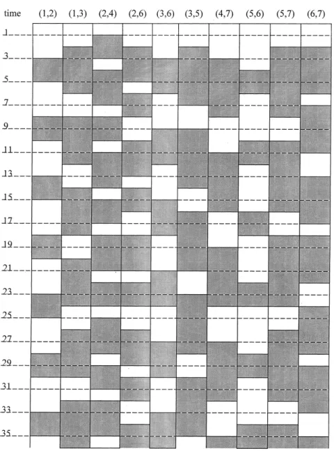
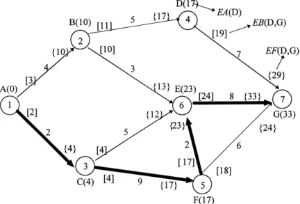
Fig. 1 shows an activity network with 7 nodes and 10 arcs, where all arcs are time-switch arcs. Activity times are shown on the arc, and the number inside each node is its topological order. Topological order is an order of nodes in an acyclic graph and can be easily constructed in time O…jAj ‡ jVj†by using the algorithm in [17], where |A| and jVjare the numbers of arcs and nodes in the network. If the topological order of nodeu is smaller than that of node v, all arcs emanating from node vcannot be predecessors to arcs ema-nating from node u. This ensures that all prece-dence relationships are satis®ed when all the activities are executed according to their topolog-ical orders. To help understand examples follow, Fig. 2 shows rest windows (plain areas) and work windows (shaded areas) of each arc ranging from 0 to 36 based on the data given in Fig. 1.

Let EA(u) denote the earliest time that all predecessors to node u are completed in a time-switch activity network. If EA(u) falls inside a work window, arc …u;v† begins just at the time EA(u) without a delay. On the other hand, if EA(u) happens to be in a rest window, arc…u;v†

cannot begin until the next work window. Owing to this, we need to develop a procedure to de-termine the earliest beginning time of arc …u;v†. Let EB…u;v† be the earliest beginning time of arc …u;v†, then the earliest ®nishing time of arc

…u;v†, denoted by EF…u;v†, may not equal to EB…u;v† ‡t…u;v†, because the activity may need more than one work window to complete. Con-sequently, we also need to develop a procedure to determine the earliest ®nishing time of arc …u;v†.

We prove a theorem (Appendix A, Theorem A.1) which validates the following algorithm for de-termining EB…u;v† and EF…u;v†. In addition, the time complexity of the algorithm is shown to be O(k) in Appendix B, Lemma B.1. To present the algorithm, we introduce variables used in the algorithm ®rst. Algorithm Earliest-Time. 1. (Initialization) LetS0ˆ0 and WS0ˆ0. Compute Siˆri‡wi‡Siÿ1 and WSiˆwi‡ WSiÿ1 foriˆ1 tok. De®ne S…nk†‡iˆ …Skn† ‡Si; r…nk†‡iˆri,

and w…nk†‡iˆwi for all positive integers n

and foriˆ1 tok.

2. (Find the earliest beginning time of arc (u,v)) 2.1. ComputenˆëEA(u)/Skûand remˆEA(u)

modSk.

2.2. Find ajsuch thatSjÿ16rem<Sj where

16j6k.

As a result,S…nk†‡jÿ16EA…u†<S…nk†‡j.

2.3. If EA…u†<S…nk†‡jÿ1‡r…nk†‡j, then

EB…u;v† ˆS…nk†‡jÿ1‡r…nk†‡j

else EB…u;v† ˆEA(u). Sk the total duration of a cycle withkpairs of

rest and work windows, i.e.,

Sbˆ Xb

iˆ1

…ri‡wi†;1 6 b 6ck

WSk the work duration of a cycle withkpairs of rest and work windows, i.e.,

WSbˆ Xb

iˆ1

wi;1 6b 6 ck

n the number of completek-pairs that EA(u) goes through

rem the remaining time after EA(u) goes throughn ofk-pairs

j rem falls inside eitherrjorwj

nw the number of completek-pairs required to ®nish arc…u;v†

rw in Step 3.1 below, it means that afternwof work, how much more time is required to ®nish arc (u,v); in Steps 3.2 and 3.3, it denotes the remaining time required to ®nish arc …u;v†

rb‡1 the rest window follows wbwhich is

executing arc…u;v†

wb‡1 the work window follows rb‡1

3. (Find the earliest ®nishing time of arc…u;v†) 3.1. Compute nwˆët(u,v)/WSkû and rwˆ

t…u;v†mod WSk. 3.2. If rwˆ0 and EB…u;v† ˆS…nk†‡jÿ1‡ r…nk†‡j; then EF…u;v† ˆEB…u;v† ÿr…nk†‡j, go to Step 3.4 If rw<S…nk†‡jÿEB…u;v†, then EF…u;v† ˆ EB…u;v† ‡rw, go to Step 3.4 rwˆrwÿ …S…nk†‡jÿEB…u;v††. 3.3. Forbˆnk‡jto…n‡1† k‡jÿ1 ifwb‡1Prw, then ifrwˆ0, then EF…u;v† ˆSb, go to Step 3.4 else EF…u;v† ˆSb‡rb‡1‡rw, go to Step 3.4 elserwˆrwÿwb‡1 Endfor. 3.4. EF…u;v† ˆEF…u;v† ‡nwSk:

4. If EF…u;v†>cSk then the solution is

infeasi-ble.

If the cycle starts with a work window, simply rede®ne Si to be wi‡ri‡Siÿ1, and modify

computations relevant to the window sequence. For example, Step 2.3 becomes: If EA…u† <

S…nk†‡jÿ1‡w…nk†‡j, then EB…u;v† ˆEA(u), else

EB…u;v† ˆS…nk†‡j. Refer to Theorem A. 1 where

modi®cations are needed.

Example 1.Consider the arc (6, 7) in Fig. 1, where

t(6, 7)ˆ8 and TS(6, 7)ˆ[1, (2, 4), (1, 4)], i.e., cˆ 1,kˆ2,r1ˆ2,w1ˆ4,r2ˆ1,w2ˆ4. Suppose that EA(6)ˆ23. By Step 1,S0ˆ0,S1ˆ6,S2ˆ11, WS0ˆ0, WS1ˆ4 and WS2ˆ8. Step 2.1 computes

nˆë23/11ûˆ2, and remˆ23 mod 11ˆ1. In Step

2.2, since 0ˆS0 6 1ˆrem<S1ˆ6, we have 22ˆS4 6 23ˆEA(6)<S5ˆ28. Consequently, EA(6) falls inside either r5 or w5. Step 2.3 tests whether EA(6) is in r5 by comparing EA(6) with

S4‡r5…ˆ22‡2ˆ24†. Since it is true (EA(6)

<24), EB(6, 7) is set toS4‡r5ˆ24.

To compute EF(6, 7), by Step 3.1, nwˆë8/ 8ûˆ1, andrwˆ8 mod 8ˆ0. Step 3.2 ®rst checks whether rw can be ®nished in w5. Since rwˆ0, which means requiring none of w5, EF(6,7)ˆ

EB(6,7)ÿr5ˆ24ÿ2ˆ22. Finally, bynwˆ1 and S2ˆ11, Step 3.4 computes EF(6,7)ˆ 22‡ 111ˆ33.

To analyze the ¯oat of the longest path in a time-switch network, we develop an algorithm similar to the two-phase procedure used in the traditional activity networks. The ®rst phase (or forward pass) is to ®nd the earliest beginning time of each nodev, EA(v), and the longest path froms to d. On the other hand, the second phase (or backward pass) is to ®nd the latest beginning time of every node v, denoted by LL(v), and analyze each arc's ¯oat. In the ®rst phase, we examine every node vaccording to its topological order in ascending sequence, and use P(v) to denote the preceding node to node v. Theorem A. 2 in Ap-pendix A validates the following algorithm for ®nding EA(v). We also show the time complexity of the algorithm to be O…jVj ‡ jEjk†in Appendix B, Lemma A. 2.

Algorithm for the ®rst phase. 1. Set EA(vi)ˆ0 for all nodes.

2. Examine every nodeviin ascending sequence of

topological order.

2.1. For every arc…u;vi†going into nodevi, do

if EA…vi†<EF…u;vi†, then EA…vi† ˆEF…u;vi†

P…vi† ˆu:

2.2. For every arc…vi;u†leaving from nodevi,

call Algorithm Earliest-Time to calculate EB…vi;u†and EF…vi;u†.

3. Find the longest path by following the prede-cessor path fromdtos.

Example 2.Using the Algorithm for the ®rst phase

to solve the activity network in Fig. 1, the applying sequence of nodes is 1, 2, 3, 4, 5, 6, 7 and the ®nal result is shown in Fig. 3, where the longest path is indicated by bold lines. If we examine node 6, we have EF…2;6† ˆ13, EF…3;6† ˆ12, EF…5;6† ˆ23, and EA(6)ˆ0. By Step 2.1, EA…6† ˆ23, because 23ˆmaxf13;12;23g. Since there is only one arc

…6;7† leaving from node 6, we only have to determine EB…6;7† and EF…6;7† by calling Algo-rithm Earliest-Time. Thus, we have EB…6;7† ˆ24 and EF…6;7† ˆ33. Remaining nodes are handled in the same way and omitted.

After presenting the algorithm for the ®rst phase, we continue to discuss the second phase. Let ®nish be the duration of the longest path (in fact, ®nishˆEA(d)). In the second phase, we ex-amine every node v according to its topological order in descending sequence. Recall that LL(v) is the latest beginning time to leave node v while completing all remaining activities by the time ®nish. Suppose nodesvjVj;vjVjÿ1;. . .;vi‡1have been examined and now we examine nodevi, where the

subscript denotes the topological order of a node. The value of LL(vi) can be de®ned as

Min

u fLB…vi;u†j…vi;u† 2Ag;

where LB…vi;u† denotes the latest time arc …vi;u†

must begin to complete all remaining activities by the time®nish.

Suppose LL(v) is given, we are to ®nd the latest time to ®nish arc …u;v† by going backward. If LL(v) falls inside a work window, the latest time to

®nish arc …u;v† is LL(v), because later than this time contradicts to the de®nition of LL(v). On the other hand, if LL(v) falls inside a rest window, the latest time to ®nish arc…u;v†may be at the end of the previous work window. Hence, a procedure is required to determine the latest ®nish time of arc

…u;v†. Let LF…u;v†denote the latest ®nishing time of arc …u;v†, then the latest beginning time of ac-tivity …u;v† may not equal to LF…u;v† ÿt…u;v† as explained in the earlier. Therefore, we also need a procedure to determine the latest beginning time of arc …u;v†. The following algorithm determines LF…u;v† and LB…u;v†. The proof and time com-plexity of the algorithm are referred to those of Algorithm Earliest-Time.

Algorithm Latest-Time.

1. Same asAlgorithm Earliest-Time.

2. (Find the latest ®nishing time of arc (u,v)) 2.1. to 2.2. Same asAlgorithm Earliest-Time. 2.3. If LL…v†<S…nk†‡jÿ1‡r…nk†‡j, then

LF…u;v† ˆS…nk†‡jÿ1else LF…u;v† ˆLL(v). 3. (Find the latest beginning time of arc…u;v††

3.1. Same asAlgorithm Earliest-Time. 3.2. Ifrwˆ0 and LF…u;v† ˆS…nk†‡jÿ1; then LB…u;v† ˆLF…u;v† ‡r…nk†‡j; go to Step 3.4 Ifrw<LF…u;v† ÿ …S…nk†‡jÿ1‡ r…nk†‡j†, then LB…u;v† ˆLF…u;v† ÿrw go to Step 3.4 rwˆrwÿ[LF…u;v†ÿ…S…nk†‡jÿ1‡r…nk†‡j†]. 3.3. For bˆ …nk† ‡j to …nÿ1† k‡ jÿ1 ifwbÿ1 6 rw, then if rwˆ0, then LB(u,v)ˆSb, go to Step 3.4 else LB(u,v)ˆSb ÿ1ÿrw, go to Step 3.4 elserwˆrwÿwbÿ1 Endfor. 3.4. LB(u,v)ˆLB(u,v)ÿnw´ Sk.

Now, we discuss the algorithm for the second phase to compute the latest leaving time for every node, and the latest beginning and ®nishing times of every arc. The proof and time complexity of the algorithm are also referred to those of the Algo-rithm for the ®rst phase.

Algorithm for the Second Phase.

1. Set LL(vi)ˆ 1 for all nodes. Set

LL(d)ˆEA(d), wheredis the destination node. 2. Examine every node vi in descending sequence

of topological orders.

2.1. For every arc (vi,u) leaving from nodevi,

do

if LL(vi) > LB…vi;u†, then LL(vi)ˆ

LB…vi;u†.

2.2. For every arc…u;vi†going into nodevi, call

Algorithm Latest-Time to calculate LB…u;vi†and LF…u;vi†.

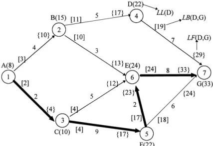
Example 3.Based on the results of Fig. 3, we use

Algorithm Latest-Time and the Algorithm for the second phase to solve the activity network in Fig. 1. Fig. 4 shows the ®nal results, where the longest path is indicated by bold lines.

3. Discussions of ¯oats

Since information about ¯oat is critical for a project manager who monitors the project to stay on schedule by adjusting budgets and allocating resources, in this section we provide a more de-tailed analysis of the ¯oat. Recall that the total ¯oat of an arc (u,v) in a traditional activity net-work is de®ned as

LL…v† ÿEA…u† ÿt…u;v†:

To have an insight into the ¯oat and study how it may a€ect the scheduling of the project when time-switch constraints are included, we decom-pose the total ¯oat of an arc (u,v) into four parts:

pre-waiting ¯oat, post-waiting ¯oat, in-waiting ¯oat and net ¯oat. Their de®nitions and calcula-tions are given as follows:

· pre-waiting ¯oat: the time we are forced to wait before begin the activity (ˆEB(u,v)ÿEA(u)), · post-waiting ¯oat: the time we are forced to wait

after ®nish the activity (ˆLL(v)ÿLF(u,v)), · in-waiting ¯oat: the time we are forced to wait

during the execution of the activity (ˆLF…u;v† ÿLB…u;v† ÿt…u;v††,

· net ¯oat: the beginning time of the activity can vary (ˆLB…u;v† ÿEB…u;v†).

It is easy to see that the following equation holds: total floatˆpre-waiting float‡in-waiting float

‡net float‡post-waiting float:

Consider the arc (4, 7) in Figs. 3 and 4, we have: EA…4† ˆ17; EB…4;7† ˆ19; LB…4;7† ˆ22;

EF…4;7† ˆ29; LF…4;7† ˆ32; LL…7† ˆ33:

Though node 4 is ready for execution at time 17, it can not be executed until the next work window, time 19. Therefore, the pre-waiting ¯oatˆ19ÿ

17ˆ2. In an analogous way, the postwaiting ¯oatˆ33ÿ32ˆ1. Suppose the activity begins at

time 22, it will ®nish at time 32 and thus the du-ration is 10. However, the actual working time is only t…u;v† ˆ7 and leaves the in-waiting ¯oat to be 3. Finally, the net ¯oat is 22ÿ19ˆ3, which indicates that we have the ¯exibility of 3 to begin the activity.

After introducing four kinds of ¯oats in the time-switch activity network, we present some in-teresting ®ndings and discuss their implications di€erent from those in a traditional activity net-work.

(1) The beginning time of an arc may no longer be a single range of continuous values but contain multiple ranges of values. Consider the arc (3, 6). We have

EB…3;6† ˆ4; LB…3;6† ˆ16:

According to the de®nition, the net ¯oat equals 12. In a traditional sense, the activity can begin in range [4, 16] without delaying the entire project. In this example, however, the allowable beginning times are in ranges [4, 6), [9, 12), and [15, 16). On the one hand, the result simply re¯ects the nature of the problem. On the other hand, it supple-ments information for e€ectively allocating the resources by properly meeting the separate schedule.

(2) The net ¯oat of an arc may not remain a constant. Consider an alternate form of de®nitions of the net ¯oat and in-waiting ¯oat:

· in-waiting ¯oat: the time we are forced to wait during the execution of the activity (ˆEF…u;v† ÿEB…u;v† ÿt…u;v†),

· net ¯oat: the ®nishing time of the activity can vary (ˆLF…u;v† ÿ EF…u;v†),

where the total ¯oat remains equal to the sum of four types of ¯oat. Interestingly, the net ¯oats in these two viewpoints could be di€erent. Consider the arc (3, 5):

EB…3;5† ˆ4; LB…3;5† ˆ10;

EF…3;5† ˆ17; LF…3;5† ˆ21:

According to the original de®nition the net ¯oat is 10ÿ4ˆ6, in contrast, the alternate form shows that the net ¯oat equals 21ÿ17ˆ4. What leads to these two values unequal is because di€erent

beginning times require di€erent work and rest windows. In this example, beginning at time 4 will ®nish the activity at time 17, while 4 out of 13 are in the rest window. In contrast, beginning at time 10 will ®nish the activity at time 21, leaving only 2 in the rest window. The result suggests that be-ginning earlier may require actual working times longer, an interesting outcome compared with a traditional model where the length of actual working time is generally insensitive to the begin-ning time. From a management perspective where the project's cost is related to the actual working time, the cost can be controlled more precisely using this information.

(3)The total ¯oat of a critical arc may no longer be zero. It is obvious from (2) the arc (3, 5) is on the longest path but with a positive ¯oat. What does it imply that a critical arc may have a positive ¯oat? From the perspective of scheduling, this ®nding suggests that a critical arc is likely to be delayable, i.e., to execute a critical activity but with relaxed time constraints. From the perspec-tive of resource allocation, it indicates that an arc on the longest path is less critical than that in a traditional one. Whether or not to pay the most attention to the critical arcs should actually de-pend on the progress or needs of the project. That is, we may execute the activities based on a priority list in order of their ¯oats.

(4)The whole system may have a system's ¯oat, because the latest beginning time of the entire pro-ject might be greater than zero. For example, Fig. 4 has the following:

EA…1† ˆ0; EA…7† ˆ33;

LB…1;3† ˆ8; LL…7† ˆ33:

Given the data, if the project begins at the earliest time 0, then it takes 33 time units to ®nish the project. However, if the project does not begin until time 8, it still can ®nish at time 33, only re-quiring 25 time units. The ®nding is in principal consistent with that of (2) above, since a project is composed of a set of activities with time-switch constraints. The implication is that we may have an option of evaluating the entire project's cost from an overall perspective without knowing each activity's detailed ¯oat.

4. Conclusions

Managing a project with e€ective allocation of budgets and resources is important in practical applications. Since time factors play a dominant role in scheduling and managing the project, fail-ure to include them not only produces misleading information but also results in incorrect decisions. In this paper, we incorporates one type of time constraint, called time-switch constraint, into the traditional network. The main results of this paper are summarized as follows.

(1) A more practical and useful model is pro-posed. In a traditional activity network, an activity is executed at any time after all of its preceding activities have been completed. In reality, however, an activity is rarely ready for execution at any time because of some forms of time constraints. Inclu-sion of such time constraints is more valuable and practical.

(2) Ecient solution methods have been devel-oped. Both the forward pass and the backward pass algorithms for determining the critical activ-ities are developed and can be run in time of O…jAj ‡kjVj†. Because of the algorithms' ecien-cy, they can be applied without causing serious computational diculties.

(3) The di€erences from a management per-spective between the traditional model and the proposed model are investigated. By decomposing the traditional total ¯oat into four components, the investigation reveals the following ®ndings: (a) the critical arcs may have ¯oats, (b) the entire project may also have the ¯oat, (c) the ¯oat of an arc may consist of multiple ranges of values, and (d) the net ¯oat of an arc can be viewed in two ways.

This paper has some possible extensions. First, the window time can be assumed to be uncertain in nature. Moreover, to re¯ect the importance of controlling the project's cost, a setup cost associ-ated with executing an activity can be considered. Finally, as discussed in the earlier section that the system may have a system's ¯oat, two interesting issues deserve further studying: (1) what is the shortest critical path in a time-switch network? and (2) when to begin the project with minimum actual time to ®nish the project?

Acknowledgements

The authors are grateful to the anonymous referees for their helpful comments.

Appendix A

Theorem A.1.LetEB(u,v)andEF(u,v)denote the

earliest beginning time and ®nishing time of arc (u,v). Then the algorithm Earliest-Time correctly ®ndsEB(u,v)andEF(u,v)for each arc(u,v)in the arc set A.

Proof.The central logic of the algorithm consists

of two parts: (1) determines the number ofk-pairs (Sk) advanced, and (2) ®nds the remaining time

and the window. To compute EB(u,v), Steps 2.1 and 2.2 obtainn, rem, andjas described in (1) and (2). Then, there are two cases.

Case 1. If EA(u) is in a work window, then arc

…u;v† can begin right away; therefore, EB…u;v† ˆEA(u).

Case 2. If EA(u) is in a rest window, then arc

…u;v† has to delay until the next work window; therefore, EB…u;v† ˆS…nk†‡jÿ1‡r…nk†‡j:

To compute EF…u;v†, Step 3.1 does (1) and (2) and obtainsnwandrw. After obtainingnwandrw, we ®rst ®nd the ®nishing time based on rw and EB…u;v†, and then add this ®nishing time to the result of multiplying Sk by nw. There are three

cases to be considered.

Case 1. If rwˆ0 and EB…u;v† ˆS…nk†‡jÿ1

‡r…nk†‡j, thenS…nk†‡jÿ1 is the end of work; there-fore, EF…u;v† ˆEB…u;v† ÿr…nk†‡j.

Case 2. Ifrw<wb (i.e., current work window),

then arc …u;v† can be ®nished in this window; therefore, EF…u;v† ˆEB…u;v† ‡rw.

Case 3. If rw>wb, then we must iteratively

search subsequent kÿ1 work windows, each by reducingrw, to ®nish arc…u;v†. In each iteration, there are two cases.

· If wb‡1>rw andˆ0, then wb is the end of

EF…u;v†; therefore, EF…u;v† ˆSb.

· If wb‡1>rw, then EF…u;v† can be ®nished in wb‡1; therefore, EF…u;v† ˆSb‡rb‡1‡rw. Finally, it is obvious the solution is infeasible if EF…u;v†>cSk.

Theorem A.2. Let EA(v) denote the earliest time that all predecessors to node v are completed.Then the algorithm for the ®rst phase correctly ®nds EA(v)for each node v in the node set V.

Proof.We prove this theorem by induction. Letv1

be the ®rst node examined in the algorithm. Obviously, v1ˆsand the theorem is true because node sis the source node. Assume the theorem is true for nodesv1;v2...;viÿ1. Now we consider node

vi whose topological order is i. For node vi, the

value of EA(vi) can be de®ned as Maxu {the earliest time arc…u;vi†reaches nodevij…u;vi† 2A}. Since EF…u;vi†found by Algorithm Earliest-Time is the earliest time arc …u;vi†reaches node vi, the

de®nition of EA(vi) can be rewritten as Maxu fEF…u;vi†j…u;vi† 2Ag. Since Step 2.1 matches this de®nition, EA(vi) is truly the earliest time that all

of the activities preceding node vi are

complet-ed. Appendix B

Lemma B.1. Algorithm Earliest-Time has time

complexity O(k),where k is the maximum number of pairs of windows in a cycle.

Proof.Steps 1 and 2.2 can be done in time O(k),

while Steps 2.1, 2.3, 3.1, 3.2, 3.4 and 4 can be done in time O(1). Because the loop in Step 3.3 iterates from bˆnk‡jtobˆ …n‡1† k‡jÿ1, the algorithm can be done in time O(k).

Lemma B.2.The time required for the ®rst phase is

O…jVj ‡ jEjk†, where k is the maximum number of pairs of windows in a cycle.

Proof. The ®rst phase examines every node one

time and every arc two times. Further, we call Algorithm Earliest-Time when initially examining each arc.

References

[1] S.E. Elmaghraby, Activity nets: A guided tour through some recent developments, European Journal of Opera-tional Research 82 (3) (1995) 383±408.

[2] K.C. Chae, S. Kim, Estimating the mean and variance of PERT activity time using likelihood-ratio of the mode and the midpoint, IIE Transactions 22 (3) (1990) 198±203. [3] J.C. Hershaur, G. Nabielsky, Estimating activity times,

Journal of Systems Management 23 (9) (1972) 17±21. [4] D.L. Keefer, W.A. Verdini, Better estimation of PERT

activity time parameters, Management Science 39 (9) (1993) 1086±1091.

[5] J. Magott, K. Skudlarski, Estimating the mean completion time of PERT networks with exponentially distributed durations of activities, European Journal of Operational Research 71 (1) (1993) 70±79.

[6] A. Nadas, Probabilistic PERT, IBM Journal of Research and Development 23 (3) (1979) 339±347.

[7] H. Soroush, Risk taking in stochastic PERT networks, European Journal of Operational Research 67 (2) (1993) 221±241.

[8] T.M. Williams, Criticality in stochastic networks, Journal of the Operational Research Society 43 (4) (1992) 353±357. [9] H.M. Soroush, The most critical path in a PERT network, Journal of the Operational Research Society 45 (3) (1994) 287±300.

[10] P.K. Anklesaria, Z. Drezner, A multivariate approach to estimating the completion time for PERT networks, Journal of the Operational Research Society 37 (8) (1986) 811±815.

[11] J. Kamburowski, An upper bound on the expected completion time of PERT networks, European Journal of Operational Research 21 (2) (1985) 206±212.

[12] P. Robillard, M. Trahan, The completion time of PERT networks, Operations Research 25 (2) (1977) 15±29. [13] D. Sculli, The completion time of PERT networks,

Journal of the Operational Research Society 34 (2) (1983) 155±158.

[14] D. Golenko-Ginzburg, D. Blokh, A generalized activity network model, Journal of the Operational Research Society 48 (4) (1997) 391±400.

[15] Y.L. Chen, D. Rinks, K. Tang, Critical path in an activity network with time constraints, European Journal of Operational Research 100 (1997) 122±133.

[16] M.M. Solomon, Algorithms for the vehicle routing and scheduling problems with time window constraints, Oper-ations Research 35 (1987) 254±265.

[17] T.H. Cormen, C.E. Leiserson, R.L. Rivest, Introduction To Algorithms, MIT Press, Cambridge, MA, 1992, pp. 485±488.