MPRA
Munich Personal RePEc Archive
Deterrence from self-protection measures
in the ‘market model’ of crime: dynamic
panel data estimates from employment in
private security occupations
Paul R. Zimmerman
US Federal Trade Commission
25. October 2010
Online at
https://mpra.ub.uni-muenchen.de/26187/
Deterrence from self-protection measures in the ‘market model’ of crime: dynamic panel data estimates from employment in private security occupations
Paul R. Zimmerman†
Abstract
Private individuals and entities invest in a wide variety of market-provisioned self-protection devices or services to mitigate their probability of victimization to crime. However, evaluating the effect of such private security measures remains understudied in the economics of crime literature. Unlike most previous studies, the present analysis considers four separate measures of private security: security guards, detectives and investigators, security system installers, and locksmiths. The effects of laws allowing the concealed carrying of weapons (an unobservable precaution) are also evaluated. Given that Ehrlich’s ‘market model’ suggests private security is endogenous to crime, the analysis relies primarily on dynamic panel data methods to derive consistent parameter estimates of the effect of self-protection measures. The relationship between self-protection and UCR Part II Index offense (arrest) data are also considered in order to provide exploratory evidence on the interaction between publicly and privately provisioned crime deterrence efforts.
Keywords: Crime, Deterrence, Market model, Private Security, Self-protection JEL Classification: K42
October 25, 2010
Copyright 2010 by Paul R. Zimmerman. All rights reserved. The views expressed herein are those of the
author and not necessarily those of the US Federal Trade Commission, its Chairman or Commissioners, or any other staff.
† Economist, US Federal Trade Commission, Bureau of Economics, Antitrust I, 600 Pennsylvania Avenue, Washington, DC, 20580. E-mail: <[email protected]>.
1 Introduction
In addition to fiscally supporting police, courts, prisons, and other publicly provided methods for deterring crime, private individuals or entities may also invest in market-provisioned self-protection devices or services to mitigate their probability of victimization. Common examples of such ‘private security’ efforts include, but are not limited to, the installation of residential burglar alarms, the use of closed circuit television (CCTV) cameras by convenience stores, and the purchase of firearms and mace.
Private security investments reflect society’s implicit ‘derived demand’ for offenses in the market model of crime (Ehrlich, 1981), and there has been a steady increase in the both the level and rate of such investments over the past several decades. For instance, in the 1970s there were 1.4 public police officers for every private security officer, but this proportion fell to just 0.33 in the 1990s (Blackstone & Hakim, 2010). Private expenditures on self-protection are now larger than public expenditures used towards maintaining the criminal justice system. Philipson & Posner (1996) estimate that annual expenditures on private protection amount to $300 billion,
although this figure does not include the opportunity cost of some private security measures (e.g.,
avoiding travel through crime-prone areas) (Ayres & Levitt, 1996).
It is well understood that private security efforts could either deter or displace crime depending on whether the investment is observable to potential offenders. Unobservable investments, such as carrying concealed handguns or installing hidden theft recovery systems in cars, might lower the probability of victimization for unprotected targets (a positive externality) since criminals cannot readily ascertain which potential victims are using the device. Overall crime rates may therefore fall in response to unobservable victim precautions. Conversely, observable precautions, such as employing uniformed security guards or installing a security system along with a sign indicating its presence, might simply displace crime to unprotected
targets (a negative externality) assuming that the uptake of such investments is not sufficiently
broad. The concomitant effect on the overall crime rate may be negligible or even positive.1
Despite the likely importance of self-protection in reducing victimization risks and the associated externalities, empirical evaluations of private security efforts (either observable or unobservable) remain sparse in the economics of crime literature. Several studies rely on
cross-sectional survey data for a specific locale (such as a city, community, or transportation system)
and often evaluate only a single type of precaution.2 Another body of literature employs
aggregate-level data and using panel methods to estimate the effect of private security on crime––
in particular, laws allowing private citizens to carry concealed weapons.3 These studies also tend
to consider only a single type of private precaution and, therefore, may also suffer from omitted variable bias if various types of self-protection are correlated with each other.
This paper contributes to and expands upon the previous empirical literature on estimating the deterrent effect of private security measures by employing a rich, public dataset
that has not been exploited in previous work.
Unlike most previous studies, the present analysis
considers four separate measures of private security: security guards, detectives and investigators, security system installers, and locksmiths––as proxied by the employment levels in each group. The effects of laws allowing the concealed carrying of weapons (an unobservable precaution) are
1 Lacroix & Marceau (1995) present a theoretical analysis wherein the adoption of an observable private
security measure may even induce crime at the protected location by signaling the presence of something valuable.
2 Hakim & Shachmurove (1996) provide evidence that burglar alarms deter commercial burglaries.
DiTella et al. (2006) (Argentinean data) find that private security guards deter the incidence of residential burglaries. Armitage & Smithson (2007) (British data) conclude that gating residential back alleys reduces crime. See Benson (1997, 1998) for cites to and discussion of earlier studies.
3
See, e.g., Lott & Mustard (1996), Ayres & Donohue (2003), and Lott (2010). Ayres & Levitt (1998) conclude that the (unobservable) Lojack anti-theft system deters auto thefts. Gonzalez-Navarro (2008) (Mexican data) reaches a similar conclusion. Benson & Mast (2001) find that some crimes are negatively correlated with the level of (possibly observable) security establishments or security personnel (in addition to concealed carry laws). Priks (2009) (Swedish data) finds that the installation of (observable)
surveillance cameras reduced crimes in subway stations with some displacement to surrounding areas. Cook & MacDonald (2010) report that the establishment of business improvement districts in Los Angeles correlate with fewer crimes and arrests without any displacement effects to adjacent areas. Vollaard & van Ours (2010) (Dutch data) find that a national law requiring the installation of burglary-proof windows and doors in new residential houses lowered the incidence of burglary with ambiguous displacement effects.
also evaluated. Since the market model suggests private security is endogenous to crime, the analysis relies primarily on dynamic panel data methods to derive consistent parameter estimates of the effect of self-protection measures. The relationship between self-protection and Part II Index offense (arrest) data are also considered in order to provide exploratory evidence on the interaction between publicly and privately provisioned crime deterrence efforts.
The paper proceeds as follows. Section 2 employs the market model to theoretically assess the relationship between self-protection and victimization risk and discusses conditions under which even observable precaution efforts may affect overall crime rates. Section 3 reviews the data while Section 4 discusses the empirical methodology for estimating the supply of crime. Section 5 presents structural and instrumental variable estimates of the effect of private security on Part I Index offenses. These results suggest that private security is in fact endogenous to crime and that some offenses are deterred by some types of private security. Section 6 turns to Part II Index arrests and shows that the relationship between public and private deterrence efforts may be dependent on characteristics of the latter. Section 7 provides concluding remarks.
2 Theoretical framework––Isaac Ehrlich’s ‘market for offenses’ model and the relationship between private security efforts and crime rates
Ehrlich (1981, 1982, 1996) extends Becker’s (1968) seminal theoretical work on modeling offender behavior to consider a ‘market model’ of crime. In this model both the propensity of offenders to enter into criminal activity on the ‘supply’ side and potential victims to ‘demand’ crime through their investments in private protection efforts are considered. Following Becker (1968), the framework also models the role of government intervention through law enforcement via a social planner’s minimization of a social loss function relating to private losses of crime (including costs associated with private security efforts) and the costs of implementing various levels of certainty and severity of punishment, which act as a ‘tax’ on criminal activity.
Potential offenders maximize expected utility, which is a function of income, by devoting
time to employment in either legal or illegal (criminal) income-generating activities.4 Expected
income earned in criminal activities is a decreasing function of the perceived risk of being apprehended and convicted by public (collective) law enforcement and the level of private precautions undertaken by potential victims to protect themselves and their property. Following Ehrlich, let
d pf
p = - (1)
represent the net gain per offense where d =d w w( , , )i l x is the expected differential gain per
offense on the margin as determined by the gross payoff from illegal activity (wi), the
opportunity cost of the offender’s time in an alternative (legal) activity (wl) and private security
taken by potential victims (x). Assume dwi >0, dwl < 0, and dx <0 (where subscripts
denote partial derivatives). The variables p and f indicate the probability of apprehension and
the expected punishment per offense, respectively.
Let O( )p denote the aggregate ‘supply-of-offenses’ schedule, which is an increasing
function of the net gains per offense, or Op ³0. Then write
( )s ( ) ( )
q =O p =O d -t , (1)
where q( )s is the quantity of crimes supplied and t = pf . The ‘derived-demand-for-offenses’ in
turn represents the average potential payoff per offense at alternative offense rates (Ehrlich, 1981
p. 309). This potential payoff , d , is the same as appears in the supply-of-offenses function and
reflects in part the level of vulnerable assets maintained by potential victims. Again, d is also a
function of victim expenditures on private security precautions. Such expenditures might include
burglar alarm systems, locks, guard dogs, safes, security guards, etc. Assume that the average
4 As in Ehrlich & Saito (forthcoming), the model assumes that (1) all offenses are of the same ‘type’; (2) all
potential offenders and victims are risk neutral; and (3) potential offenders and victims are distinguished by initial income levels; specifically, offenders have comparatively lower wealth levels and legitimate
perceived victimization risk is a function of the realized crime rate (Ehrlich, 1996 p. 49), or
( )q
x = x , which represents the demand function for optimal private security. Equilibrium
expenditures on private security efforts are increasing in the perceived victimization risk, or 0
q
x ³ . Substituting x( )q into d gives
( )
( d )
d =D q , (2)
such that Dq( )d £0.
Equilibrium in the market model is determined where
s d
q( ) =q( )
.
(3)Let q*denote the crime rate that implicitly solves equation (3), which corresponds to the solution
of a fixed-point problem (Ehrlich & Saito, forthcoming).5 The equilibrium of the virtual market
model of crime may then be characterized as
* ( ( )* ( ))*
q =O D q -t q . (4)
Of primary interest here is examining the comparative statistics results associated with an
exogenousincrease in private security efforts independent of any changes in public enforcement
or any change in the crime rate itself. For example, such exogenous variation may stem from technological advances in private security systems or changes in regulations governing the private security industry.
Let d* ºD q( )* , which upon substitution into equation (4) gives rise to the following
result.
Result 1. An exogenous increase in the level of (per-capita) private security expenditures results in a non-positive change in the equilibrium crime rate.
Proof: Applying the envelope theorem to equation (4) gives
5 An equilibrium solution is ensured to exist so long as D(0)-pf ³0, and the equilibrium will be unique
so long as dO( )/p dq =D Oq p <0, i.e., the net return from crime turns negative as the crime rate rises above its equilibrium value (Ehrlich & Saito, forthcoming).
* * * * ( )( ) 0 1 ( ) 1 O d q d q x t x ¶ ¶ + -¶ = ¶ ¶ = £ ¶ ¶ + + + ¶ . ■ (5)
Result 1 demonstrates, all else equal, that an exogenous increase in private security precautions
lowers the equilibrium offense rate, i.e., effectuates a deterrent effect. The various partial
derivatives in equation (5) inform the magnitude of the deterrent effect. Ceteris paribus, the
deterrent effect will be larger (i.e., more negative): (1) the more elastic the supply-of-offenses
function with respect to the expected differential gain per offense; and (2) the greater the
(negative) impact of private security efforts on the expected differential gain per offense.6
Furthermore, the deterrent effect of private security will be smaller the greater the response of public enforcement to increases in the crime rate.
Since the optimal private security function is increasing in the crime rate, it is possible that observed changes in private security efforts (or expenditures) could be positively correlated with observed changes in crime. Indeed, this is the same type of endogeneity bias that confounds empirically indentifying the deterrent effect of police or incarceration rates in aggregate data. The endogenous relationship between crime and private security can be readily demonstrated in the context of the market model considered above.
Consider Figure 1. Assume there is no instantaneous impact of a change in the level of per-capita private security efforts on any public enforcement efforts. Suppose there is an
exogenous decrease in wl due to, say, an unexpected labor demand shock that lowers ‘legitimate’
wages; thus wl,0 >wl,1. This change, operating through a positive effect on d0, shifts both the
6 These results can also be seen by rewriting equation (5) in elasticity form:
O q e q e * , , 1 x t x ¶ = ¶ + ,
where eO,x <0 denotes the elasticity of the supply of offenses with respect to private security efforts and q
et, >0 the elasticity of public enforcement efforts with respect to the crime rate. This expression is
arguably more relevant from an empirical perspective since data on d are rarely available or, for some offenses (e.g., murders committed as part of so-called ‘crimes of passion’), not even observable.
initial supply-of-offense (p0) and derived-demand-for-offenses (d0 =D q0( d,0)) schedules to
the right and puts upward pressure on the equilibrium crime rate. In response, potential victims
increase their expenditures on private security (x1 > x0) since, by assumption, xq ³0. But an
increase in (per capita) private security expenditures, because of its negative effect on d, would
shift the supply and demand schedules to the left. Thus, a decrease in wl simultaneously exerts
both a ‘direct’ outward shift (through d) and an ‘indirect’ inward shift (through x) of the supply
and demand schedules in the market model.
However, as shown in Figure 1, the net effectof the countervailing shifts in supply and
demand, however, will still be a rightward shift in both curves. The equilibrium crime rate
increases from Q0 to Q1 ( *
0
q to *
1
q ). Furthermore, at Q1 optimal private security expenditures
must be greater than at point Q0 since xq ³0 and * *
1 0
q >q . These effects also necessarily
imply that d1 >d0 (or p1 > p0) at point Q1. These results are formally proved below.7
Result 2. An exogenous decrease in the opportunity costs of committing crime necessarily results in d1 >d0, which implies an increase in both the equilibrium crime rate and the level of (per capita) private security expenditures.
Proof: With little loss in generality, following Ehrlich (1996, n. 4) let d0 and d1take the
following functional forms:
0 ,0 ,0 0 1 ,1 ,1 1. i l i l d w w d w w x x = - -= - - (6)
Assume that the gross payoffs from crime are unchanging, or wi,0 =wi,1. An exogenous
decrease in the legal wage implies that
,1 ,0
l l
w <w (7)
and, ceteris paribus, shifts the net returns schedule to the right, or d1 >d0. A new equilibrium is
established at Q1 (see Figure 2). By assumption x1 >x0 at Q1 since the
derived-demand-for-offenses schedule is increasing in q. But suppose instead that
d1 £d0 (8)
following a decrease in the legal wage, which implies that the equilibrium crime does not increase
relative to its initial value. Rewrite equation (8) as
7 The same effect would apply to a change in any other variable that parameterizes the market model and
increases the net returns to crime (or vice versa). The present discussion focuses on a decrease in legal wages only for the sake of demonstration.
i l i l i i l l l l l l w w w w w w w w w w w w ,1 ,1 1 ,0 ,0 0 ,1 ,0 ,1 ,0 1 0 ,1 ,0 1 0 ,0 ,1 1 0 ( ) ( ) ( ) 0 0 0 x x x x x x x x - - £ - - - - - £ - + - + £ - £ (9)
It must be the case that x1 £x0 if equation (9) is satisfied. Substituting this condition into
equation (10) shows that its inequality constraint can only be satisfied if w,1 £w,0, which is a
contradiction. ■
The analysis in Figure 1 and above suggests that it might be the norm rather than the exception to empirically observe a positive correlation between private security and crime. Such observation, however, would not reflect the effect of security on crime but rather their joint determination. Indeed, Clotfelter (1978) finds that the probability of adopting private security is positively correlated with the probability of victimization for almost all of the self-protection efforts he considers, so endogeneity is a real concern from an empirical perspective. Determining the actual causal effect of private security on crime requires identifying the supply-of-offenses schedule off of shifts in the derived-demand-for-offenses schedule induced by factors that are strictly exogenous to the market model. Any empirical evaluation of deterrence from private security efforts must therefore take into account the potential endogeneity between security and crime.
2.1 Observable private security efforts and the market model of crime
The market model of crime presented above implicitly takes potential victims as
homogeneous (i.e., in an ex ante sense). This assumption implies that, in equilibrium, all
potential victims will invest in the same level of private security efforts. Any changes in crime rates stemming from increased private security efforts or expenditures therefore correspond to ‘general’ deterrence, or reductions in overall crime stemming from fewer offenses being committed against both protected and unprotected targets.
The recent theoretical (Shavell, 1991; Hui-Wen & Png, 1994; Helsley & Strange, 1999, 2004) and empirical literatures on private security focus on unobservable protection efforts such
as the carrying of concealed weapons or the use of hidden theft recovery systems (e.g., Lojack).8
These precautions could result in general deterrence because of the positive externality that arises from criminals being unable to determine which potential victims have actually adopted the effort. Observable private security efforts, such as a sign indicating the presence of a burglar alarm system, may protect the specific target employing them, but criminals might simply divert their efforts towards visibly unprotected targets. As a result, aggregate crime rates, which are the focus of the market model, might not be affected by the adoption of such precautions.
Benson & Mast (2001), however, posit several theoretical avenues by which even highly
visible private security efforts may still effectuate general deterrence and, therefore, be evaluated
under the market model. First, if observable private security efforts result in criminals diverting
their efforts between protected and unprotected targets, entrepreneurs may recognize new sales opportunities and offer more security services to potential targets. If such entrepreneurial efforts are successful, the number of protected targets with observable security efforts could expand over time, perhaps to an extent that “the expected cost of searching for targets and/or committing
crimes could rise, making potential criminals less likely to become actual criminals.”9
Second, sellers of private security services may be unable to exclude some non-payers
from reaping some benefits of the sales made to other customers. For example, some potential crime victims may be able to take advantage of observable security investments made by others,
and if so, then general deterrence effects may arise as a positive externality. Benson & Mast (p.
730) note:
Firms in a shopping or entertainment area may employ security primarily to prevent shoplifting, vandalism, and employee theft, for instance, but a potential victim of robbery or rape may choose to shop or socialize in that area to take advantage of the security presence. If a substantial portion
8
See supra notes 2 and 3 for cites to recent empirical studies.
9 Benson & Mast (2001). DiTella
et al. (2006) present evidence that suggests the adoption of private security by higher-income households leads to more crime being diverted to lower-income households, who tended to adopt private security and a much smaller rate. An implication of this finding is that if lower-income households could afford private security (or where provisioned with it through government subsidy), then the displacement would not have occurred, which is consistent Benson & Mast’s argument. See also Cook & MacDonald (2010, p. 14: “If adoption of effective technology is broad enough, the scope for displacement . . . is limited.”).
of potential victims behave this way, robberies and/or rapes could be reduced because the cost for potential criminals of finding an easy target is higher.
Third, purchasers of observable security efforts might recognize the presence of the
above positive externalities and internalize them, e.g., by incorporating the cost of providing a
secure environment into the price charged for the final product, such as a higher ticket price at a movie theater. In this case “[t]he general deterrence impact could still arise, but it would be paid
for by those who benefit from it.”10 And fourth, some ostensibly ‘observable’ private security
efforts, such as plainclothes security guards or detectives, could in fact be difficult for potential criminals to detect. Uncertainty about where such security efforts are deployed could lead to a
general deterrence effect.11
Cook & MacDonald (2010) also offer some insights into how observable precautions might induce general deterrence. Criminals may be heterogeneous in their skills, and observable precautions may affect unskilled criminals more than skilled ones. For instance, use of a steering wheel lock may lower aggregate auto theft rates by deterring many ‘joyriding’ thefts (which tend to be committed by younger, less experienced criminals) but have little effect on the behavior of higher-skilled professional car thieves who fence auto body parts. Owners of higher-valued vehicles (or property in general) may also be more likely to adopt security measures, thereby forcing criminals to divert their efforts towards less lucrative unprotected targets. If the return from committing crime against these latter targets is sufficiently low, criminals may be better off seeking out legitimate employment.
In summary, the potential for even ‘visible’ private security efforts to induce general (as well as specific) deterrence allows even these types of precautions to be analyzed in the general context of the market model. The following section discusses data that can be used to
operationalize the market model in order to empirically evaluate the relationship between private security efforts and crime.
10 Benson & Mast (2001).
11
3 Data
Previous empirical research on private security efforts and crime have relied on both level data (obtained from surveys) and aggregate-level data. While some individual-level studies may consider a number of private security efforts, the data are typically measured at a single point in time. The cross-sectional estimates obtained from these studies may not control for a variety of unobservable factors that may influence both crime rates and the propensity to adopt private security, thereby leading to biased inference. Furthermore, the extent to which the results from these studies may generalize to other groups periods (be they proximate or
otherwise) is uncertain.
Aggregate-level studies, which typically employ pooled cross-section time series (panel) data, have allowed researchers to better control for omitted variable bias through estimation of fixed effects models. These studies, however, have not controlled for the wide range of private security efforts due to data limitations. Benson & Mast (2001) use county-level data obtained
from the US Census Bureau’s County Business Patterns (CBP) dataset, which reports the number
of establishments specializing in ‘security and detective services.’ However, the CBP dataset does not contain measures of any other forms of private security.
This study employs aggregate state-level data compiled by the Bureau of Labor Statistics (BLS) on private security efforts that have not been considered in previous studies. The data are
collected in the Occupational Employment Statistics (OES) series. The OES dataset provides
estimates of the number of persons employed (and wage estimates) for approximately 800
occupations based on a series of establishment-level surveys.13 Unlike the CBP dataset used by
Benson & Mast (2001), the OES dataset reflects employment in private security occupations
13 The OES dataset classifies an ‘employee’ as any full- or part-time worker paid a wage or salary. The
dataset does not reflect the self-employed, owners and partners in non-incorporated firms, household workers, or unpaid family workers. See BLS (2010) for further details.
outside of those firms specializing in providing security services. For example, some private retail establishments (such as department stores) may maintain their own security personnel rather than contracting out for such services. Similarly, various government agencies might recruit, train, and retain their own security personnel rather than rely on a specialized private security firm.14
The OES dataset also goes beyond the CBP dataset in that they measure employment in
several relevant occupations. 15 The CPB dataset groups together private guard and detective
services, which is a potential shortcoming since the duties performed by those two employment groups are quite different. Annual OES employment estimates are separately available for security guards, private detectives and investigators, security and fire alarm system installers, and locksmiths and safe repairers. Employment trends in these occupations should reflect variation over time in the extent those private security efforts are acquired and deployed by end users
across states.16
Private security services and devices are, of course, employed across a wide range of industries. Table 1 presents national-level employment estimates for the five largest industry employers of each OES private security group. Not surprisingly, the single largest employment industry is ‘investigation and security services,’ which comprises about 79.7 percent of the
employment in those industries listed in Table 1.17 ‘Government’ (including schools) is the
14 These data have not been widely used in academic studies; the majority of their (few) econometric uses
have been in the labor economics literature. See, e.g., Dey et al. (2009), Dey & Stewart (2008), and Abraham & Speltzer (2010).
15 The OES does not release state-level occupation-specific employment estimates by industry (such
estimates are available only nationally). Thus, one cannot determine the number of, say, security guards employed within retail establishments at the state level.
16 Employment levels for private guards and detectives will obviously represent the extent to which those
efforts are directly acquired and deployed by the purchasers of those services. The relationship between employment and deployment levels pertaining, e.g., to alarm systems may be somewhat less direct, but changes in employment levels are still likely to reflect changes in the extent to which alarms, security systems, safes, etc. are purchased and utilized by end users (the estimated effects of private security on crime are identified off of within-state variations in these measures).
17 This figure is likely biased upward (and all others downwards) since the OES data are effectively
capturing counts of employees that are ‘directly’ employed by each industry. It is almost certain that many of the persons counted in the ‘investigation and security services’ industry are actually deployed in other
second largest, comprising about 9.3 percent. Other notable industries include ‘legal services’ in the case of private detectives and investigators and ‘hospitals’ in the case of locksmiths and safe repairers.
While the OES dataset clearly provide several distinct advantages, Abraham & Speltzer
(2010) highlight several issues that may hinder its application to any econometric analyses
relying on the time series dimension of the data.18 Before 1996 establishments in specific
industries were surveyed on a three-year rotating cycle, but since then all industries are sampled in each year. However, save for the federal and state government ‘industries,’ the largest establishments within each industry are still surveyed only once every three years.
OES employment estimates for a given year are derived from panels of establishment surveys taken over prior years to ensure that large establishments are sampled. Prior to 2002, estimates were based on the current year’s survey panels plus the previous two year’s (each panel consisting of about 400,000 establishments across all industries), with establishments assigned an October, November, or December reference date. Beginning in 2002, the OES survey moved to a design using six semi-annual panels (each consisting of about 200,000 establishments) with each
establishment assigned a May or November reference date.19 As such, ensuring that a given
year’s estimates reflect the largest establishments in a given industry comes at the cost of those estimates not reflecting data pertaining exclusively to that year (which in turn makes it less likely
industries (e.g., government) through outsourcing (contracting with security firms). Regardless, these data may give a rough approximation of the rank order (i.e., in terms of employment intensity) of those
industries (outside of ‘investigation and security services’) that employ and outsource private security services.
18 Indeed, the BLS does not ‘encourage’ using OES data for conducting time series analysis and urges
researchers that choose to do so “to note the changes in survey procedures and the limits of the methods used with a pooled sample” (BLS 2010). As discussed herein, it does not appear that these changes have had a large effect on the estimates for the occupational classes considered in this analysis, and the BLS acknowledges that “comparisons of occupations [over time] that are not affected by classification changes may be possible if the methodological assumptions hold.” (Id.) Furthermore, the econometric methodology employed herein (which relies on panel data methods as opposed to pure time series analysis) should help to account for some of the shortcomings in the OES data (bearing in mind the BLS’s warnings regarding these methods).
19 So,
e.g., based on the current OES sampling design, annual estimates pertaining to May, 2008 are derived from data for the ‘current panel’ (dated May 2008) and the five previous panels (November 2005, May 2006, November 2006, May 2007, and November 2007), for six semi-annual panels in total.
that the data are able to capture actual year-to-year changes). The estimates, however, are benchmarked to the average of the most recent May and November employment levels.
Changes in industry classification schemes used in constructing the OES dataset may be another problem. In 1999, the OES survey changed from its own survey-specific occupational coding system to the Standard Occupational Classification (SOC) system, and in 1999 it changed from the Standard Industrial Classification (SIC) system to the North American Industry
Classification System (NAICS). These changes may make it difficult to make meaningful comparisons in the OES employment estimates over time. For example, only about half of all surveyed establishments could be assigned NAICS codes based upon their earlier SIC
classification (Abraham & Speltzer, 2010).
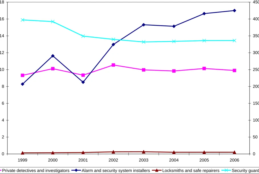
This study uses OES data beginning in 1999, which corresponds to the earliest year for which employment estimates for all four of the above-mentioned private security occupations are available, through 2006. Figure 2 graphs the national-level OES employment levels for the four private security occupation classes over the sample period. Most of the series display a relatively stable pattern over the sample period, suggesting that the changes in the occupational
classification schemes underlying the OES survey in 1999 and 2002 did not have a large effect on these employment estimates. The exception is the alarm and security system installer series. In the first three years of the sample (1999-2001) there is a marked peak in the series that occurs in 2000. Variation in the number of state cells containing employment estimates over these years appears to explain some of this movement. Data are available for 22 states in 1999, but this number increased to 38 states (an increase of 72 percent) in 2000. In 2001, however, the number of state-cells with usable observations then falls to 32.
There is a noticeable upward trend in the alarm and security system installer series after 2001. One possible explanation for this effect is the adoption of the NAICS system by the OES
in 2002. However, this explanation does not seem especially compelling given the smoother year-to-year patterns in the other series. Another possible explanation is that the September 11, 2001 terrorist attacks increased demand for private security, especially the demand for security
and alarm systems. 21
4 Empirical specification
Let j index the four OES private security occupation groups. The basic linear regression
model (which corresponds to the supply-of-offenses schedule in the market model) takes the following dynamic, double-logarithmic form:
j j i t i t j i t i t i t i t i t i t O O PrivSec CCL D X ( ) ( ) , , 1 , , , 1 , , ln ln (ln ) ln , a b g d q l e -= + + + + Y + G + + +
å
(10)where a and ei t, denote the constant and random error term, respectively. The subscript
i ={1, , 51} indexes states (including the District of Columbia) and t ={1999, , 2006}
years. The variables qi and lt denote vectors of state and year indicators, respectively.22 Table
2 presents descriptive statistics for select covariates used in estimating equation (10). These variables are discussed further below.
The dependent variable, Oi t, , denotes the reported number of Uniform Crime Report
(UCR) Part I offenses per 100,000 state residents. Oi t,-1 is the once-lagged value of the
dependent variable, which is employed as a regressor. Part I offenses consist of both violent (murder, rape, robbery, and aggravated assault) and property (burglary, larceny, and auto theft) crimes. Specifications using total violent or property offenses are not considered since the former
21 Dain & Brennan (2003) discuss the increasing liability of property owners for failing to provide security
to patrons following the September 11, 2001 attacks.
22 State-specific time trends are not included in the regression model for two reasons. First, given that
relatively short length of the panel, inclusion of these trends along with state and year indicators would likely over-parameterize the regression equation, reducing the efficiency of the estimates. Second, as discussed below, there is a concern with instrument proliferation when using dynamic panel data estimators; dropping state-specific trends reduces the instrument set considerably.
is dominated by assaults and the latter by larcenies; there is also little or no reason to weigh the individual crime categories equally.
The variable Di t,-1 denotes a vector of ‘public’ deterrence variables, which––according
to the market model (see equation (5))––may influence the impact of private security. These
measures include per-capita measures of police employment and prisoners (i.e., the incarceration
rate) as well as offense-specific arrest rates. These variables are lagged one year to mitigate
simultaneity bias. The variable Xi t, is a vector of other covariates typically included in crime
studies (per-capita income, population density, poverty rate, unemployment rate, and percent
black).23 All other Greek letters denote (vectors of) coefficients to be estimated.
The variable PrivSeci t( ),j denotes employment in the jth OES private security group,
expressed on a per-capita basis. The b( )j coefficients represent the associated crime rate
elasticity measured with respect to a one percentage point change in the jth employment class.
An estimate of b( )j that is negative and statistically significant is interpreted as evidence of a
(general) deterrent effect of that private security effort.
Another private precaution taken against crime is the ownership of weapons, particularly handguns. Allowing private citizens to carry concealed (unobservable) handguns may induce general deterrence. A large and contentious empirical literature debates the efficacy of concealed carry laws (CCLs) in reducing crimes, with some studies finding large negative effects (consistent
with deterrence) and others finding no effects or even positive effects.24 Following this
literature, equation (10) includes a dummy variable reflecting the presence of a law allowing citizens to carry concealed handguns. This variable takes a value of one in the first full year following the legal adoption of the law and in each subsequent year the law is in effect.
23 The logarithmic transformation is applied only to per-capita income and population density and not to the
other measures in Xi t, since they are defined in percentage terms.
24
5 Estimation results
5.1 Treating private security as exogenous to crime
Equation (10) is estimated via Newey-West regression, which takes the private security (and all other) variables as conditionally exogenous. The Newey-West estimator provides test statistics that are robust to heteroskedasticity and autocorrelation of arbitrary form. In
implementing the estimator, the maximum order of significant autocorrelation in the error terms is set equal to one.
Table 3 presents the estimation results. The elasticity estimates for private guards are consistently negative and statistically significant in the burglary and larceny specifications. A one percent increase in per-capita private security guards is associated with a 0.8 percent decrease in per-capita burglaries and larcenies. The estimated elasticity on private detectives is negative in five out of the seven specifications, but none of these estimates is statistically significant at conventional levels. There are also no statistically significant estimates pertaining to security system installers or locksmiths. The estimated elasticities pertaining to security system installers (locksmiths) take a negative sign in only four (three) specifications. The CCL coefficient takes a
positive sign in each specification and is statistically significant for murder, assault, and burglary.
This finding may suggest that CCL laws increase crime or that such laws tend to be passed in states with high crime rates.
The other coefficient estimates are generally consistent with expectations. The lagged dependent variable is positively and significantly correlated with crime in all specifications except murder. The (lagged) per-capita police employment elasticities are negative in five out of the seven specifications and statistically significant for robbery and auto theft. A one percent increase in the (lagged) police rate is associated with a 0.32 (0.30) percent decrease in per-capita robberies (auto thefts).
The (lagged) incarceration rate is negatively correlated with crime in only three cases. The incarceration elasticity is negative and statistically significant in the murder specification and
positive and statistically significant in the auto theft specification. One possible explanation for these ‘perverse’ positive estimates (as well as those associated with the police rate and arrest rate) is that lagging the incarceration rate does not adequately control for simultaneity bias. For instance, residual autocorrelation in the error terms disqualifies the use of deterrence lags to address endogeneity, which might explain in part the positive and/or statistically insignificant estimates on the various deterrence measures.
5.2 Treating private security as endogenous to crime
The theoretical framework considered in Section 2 and some of the previous results suggest that Newey-West estimates of private security effects could be inconsistent as they do not address the potential underlying endogeneity bias. Determining the uncontaminated causal effect of private security effects on crime therefore necessitates ‘breaking’ the simultaneity between crime and private security, or employing an empirical strategy that exploits exogenous shifts in the derived-demand-for-crime schedule in order to identify the supply-of-offenses schedule.
While many studies in the empirical economics of crime literature address endogeneity concerns (whether they be in regard to deterrence, labor market, or other factors), an ongoing difficulty with these efforts is the identification of appropriate instrumental variables. In this
regard, recent studies in this literature (e.g., Moody & Marvell 2008, Saridakis & Spengler 2009)
employ so-called ‘dynamic GMM’ estimators developed, inter alia, by Holtz-Eakin et al. (1988),
Arellano & Bond (1991), Arellano & Bover (1995), and Blundell & Bond (1998). These
estimators rely on instruments ‘internal’ to the model (i.e., the instruments are derived as lagged
levels or lagged differences of the endogenous regressors), which obviates the need to ‘find’ instruments (assuming any exist). Statistical tests can then be conducted to explore the performance of the instruments in terms of their validity and relevance. Dynamic GMM estimators are also specifically designed to address a number of econometric and data issues
relevant to this study25–– in particular, the dynamic bias in fixed effects models with lagged dependent variables (Nickell, 1981). The potential for dynamic bias that is particularly relevant to the panels with a large number of groups relative to periods, as is the case here. Dynamic GMM estimators account for this bias by also instrumenting the lagged dependent variable.
The predominant dynamic GMM estimators are ‘difference-GMM’ and ‘system-GMM.’ The difference-GMM estimator applies lagged levels of the endogenous variables as instruments in a first-differenced fixed effects model. System-GMM combines the first-differenced model with the same model in levels and uses lagged differences of the endogenous variables for the differenced equation.
Although the system-GMM is asymptotically more efficient relative to difference-GMM, the difference-GMM is preferable in the present context. The system-GMM estimator requires that the instruments are uncorrelated with unobserved state fixed effects––a condition that is met if the time series is stationary. In principle, panel unit root tests could be employed to determine stationarity, but such tests would be expected to be very low-powered with the use of only six years of data. Since difference-GMM, by definition, relies on a first-differenced specification, all
nonstationary variables are transformed to stationary ones (assuming they follow an I(1)process),
thereby making the estimator less sensitive to initial conditions.
Inference with dynamic GMM estimators is affected by the instrument count (Roodman, 2008, 2009). The number of instruments generated using these methods is increasing in the time (and group) dimension of the panel, and inference in finite samples is biased when the number of
instruments becomes ‘large’ (i.e., approaches the sample size). The relative efficiency of
system-GMM is achieved in part through the use of additional instruments. Given the relatively short
25 Specifically, these estimators are applicable to applications involving: (1) ‘large
N, small T’ panels; (2) a linear functional relationship; (3) a single dynamic, left-hand-side variable (which depends on its own past realizations; (4) independent variables that are not strictly exogenous (i.e., correlated with past and possibly current realizations of the error); (5) fixed group effects; and (6) heteroskedasticity and autocorrelation within (but not across) groups (Roodman, 2009). All of these aspects are applicable in the present case.
time dimension of the panel and only 51 potential groups,26 difference-GMM is likely a better option relative to system-GMM for obtaining valid inference.
Table 4 presents one-step difference-GMM estimates of the relevant analog to equation
(10).27 All four private security measures are treated as endogenous variables. In addition, the
CCL law, police rate, prison rate, crime-specific arrest rate, and lagged dependent variable are
assumed to be endogenous or predetermined, so all of these measures are instrumented as well.28
The ‘GMM-style’ instruments for the various endogenous and predetermined measures are their respective lagged levels. The maximum number of the relevant lags is set to two in
order to restrict the size of the instrument set.29 Following standard practice, all other covariates
used in estimating equation (10) (which are assumed to be strictly exogenous) are used as
additional (non-excluded) instruments.30
5.2.1 Evaluating the instruments
Before proceeding to the point estimates, consider the regression diagnostics given at the
bottom of Table 4. All seven models are statistically significant (as indicated by the F-statistics).
Although there are more instruments than groups (which is not the ideal), the difference is not very large. Either the Sargan or Hansen test can be used to evaluate the overidentifying
26 Because of missing data, the number of groups available for estimation is less than 51. This fact also
suggests favoring the use of difference-GMM to economize on instruments.
27 The covariance matrix of dynamic GMM estimators can be obtained through the ‘one-step’ or ‘two-step’
option (see Roodman, 2009 for further details), the latter being asymptotically more efficient. Arellano & Bond (1991) use Monte Carlo methods to show that two-step estimation of the difference-GMM model results in severely downward biased standard error estimates. Windmeijer (2005) offers a correction, but in the instant case this approach resulted in many models failing to estimate, thereby forcing reliance on the one-step estimator. Blundell & Bond (1998), however, show that one-step standard errors are virtually unbiased for moderately sized samples. Furthermore, the estimated standard errors on all the difference-GMM estimates presented herein are obtained using a cluster-robust correction, with the clustering applied to the group (state) level.
28 It may be that some of the deterrence measures are not endogenous to some crime measures. For
instance, because murders comprise only a small portion of incarcerated offenders, it may be more accurate to regard prison population as exogenous in the murder regression. Nonetheless, the same treatment is applied across the specifications for the sake of comparison and consistency.
29 Another way to reduce the number of instruments is to ‘collapse’ them (Roodman, 2009). However,
restricting the lag lengths resulted in a smaller set of instruments.
30 The state fixed effects are netted out due to differencing, and as such, state dummies are not used in the
restrictions; however, the former is less susceptible to bias resulting from using a larger
instrument set.31 The Saragn test is significant in the rape, assault, and auto theft regressions,
which suggests potential model misspecification. As such, these three models will not be discussed further.
Arrelano & Bond (1991) note that serial correlation in the idiosyncratic error term ei t,
may cause some of the lagged instruments to be invalid. The authors develop a test serial
correlation that is applied to the differenced residuals. First-order (AR(1)) serial correlation is
expected in the differenced residuals, and this result is borne out in the murder and larceny
regressions. However, the AR(1) test is not particularly important because the validity of the
instruments depends on whether there is serial correlation in the levels of the residuals, which can
be determined by testing for AR(2) in the differenced residuals. This latter test is insignificant in
all cases, which indicates that the instruments are not rendered invalid from serial correlation. Instruments must be relevant in addition to being valid. Bobba & Coviello (2007, p. 303) note that:
In a multivariate panel data framework it is not clear how to test for weak instruments, hence we use the known bias in Difference GMM by comparing its sample performances with alternative estimators with known properties in dynamic panel data . . . .
Specifically, following a procedure suggested by Bond et al. (2001), Bobba & Coviello test for
weak instruments in difference-GMM by comparing its estimated autoregressive coefficient (i.e.,
the coefficient estimate on the lagged dependent variable) with corresponding within-group (lower bound) and pooled (upper bound) estimates. If the difference-GMM autoregressive coefficient is smaller than the within-group estimate, then the difference-GMM estimator is likely
31 The Hansen test is severely weakened (meaning that it will fail to reject a false null hypothesis) when the
instrument count is relatively large. According to Roodman (2009), a Hansen-test p-value of even 0.25 with a relatively large instrument set could be indicative of weak test. In the present case, the estimated p -values for the Hansen test were well above this level (in some instances taking ‘perfect’ 1.0 value, which Roodman characterizes as a ‘telltale’ sign of a weak Hansen test). It is thus unlikely that the Hansen test can be relied upon for these estimations. And although the Sargan test (unlike the Hansen test) is not robust to heteroskedasticity, this problem is likely to be of relatively less importance here, and as such, the Sargan test is reported for all estimations.
to be seriously downward biased. This result would suggest that the instruments are only weakly
correlated with the endogenous regressors (Bond et al. 2001, p. 7).
The difference-GMM autoregressive coefficients in Table 4 all lie between their respective lower and upper bounds. This finding suggests that there is no weak instruments problem affecting the difference-GMM estimates and, therefore, that those estimates do not suffer from (downward) finite sample bias. The following subsection further evaluates the difference-GMM estimates.
5.2.2 The difference-GMM estimates
The top portion of Table 4 presents the difference-GMM estimates. Again, all reported t
-statistics reflect standard errors adjusted for generalized heteroskedasticity and autocorrelation. First consider the murder regression. While none of the Newey-West private security
employment estimates were statistically significant, the instrumented private detectives and investigators elasticity remains negative ( = -0.15) and is almost four times larger in magnitude relative to the Newey-West elasticity. Furthermore, the difference-GMM estimate of this elasticity is statistically significant at the 1 percent level with instrumenting whereas the Newey-West estimate is insignificant. As suggested by the market model, the Newey-Newey-West estimate
might suffer from endogeneity bias that operates in a positive direction (e.g., higher murder rates
may result in greater employment of private detectives and investigators). On the other hand, instrumenting causes the security guard and alarm system elasticities to turn from negative to positive, although both estimates remain statistically insignificant.
Similar to the Newey-West results, none of the difference-GMM private security employment estimates are statistically significant in the robbery regression. However,
instrumenting results in the estimated security guard and private detective elasticities to become more negative. The security alarm elasticity turns from positive to negative after instrumenting. The locksmith elasticity remains positive and is larger in magnitude than the Newey-West estimate, but it is still statistically insignificant. While these results, of course, should only be
regarded as tentative, they also suggest that the Newey-West estimates may suffer from simultaneity bias.
The difference-GMM security guard elasticity in the burglary regression remains negative and is 1.8 times larger in magnitude relative to the Newey-West estimate. The former estimate is no longer statistically significant (just missing the 10 percent significance level). The
private detective and alarm system elasticities are larger (i.e., more negative) than their
Newey-West counterparts, although these estimates are also not statistically different from zero. The locksmith elasticity remains positive and increases in magnitude after instrumenting, but is again found to be statistically insignificant.
Now consider the larceny regression. The security guard elasticity remains negative ( = -0.28) and statistically significant at the 5 percent level after instrumenting. However, the difference-GMM point estimate is 3.7 times larger in magnitude relative to the Newey-West estimate. Surprisingly, the private detectives elasticity remains positive after instrumenting and turns statistically significant at the 10 percent level. On the other hand, the magnitude of the alarm system and locksmith elasticities falls after instrumenting, but both estimates remain statistically insignificant.
The Newey-West estimates of the impact of CCLs were consistently positive, and in three specifications the coefficient estimates were statistically significant. However, after
instrumenting six of the seven CCL coefficient estimates turn negative (the exception is robbery), but all are statistically insignificant. These results suggest that CCLs may be endogenously related to crime rates, and as such, it may be necessary to instrument the law indicator in order to
derive a consistent estimate of effect of these laws.32 Instrumenting the other deterrence
variables has modest effects on their estimated elasticities (although in most instances the
32 Lott & Mustard (1997) present some results where the CCL dummy is instrumented and find that this
treatment results in more negative impacts of the law’s effect. Most studies that find a positive (crime-enhancing) effect of CCLs (e.g., Ayres & Donohue 2003) do not attempt to instrument the law. If the results presented here are any indication, such positive effects might reflect endogeneity bias rather than any tendency for CCLs to stimulate crime.
estimates move in the expected downward direction) and, with few exceptions, relatively little impact on the precision of those estimates.
6 An analysis of UCR Part II Index offenses
While the results of the previous section suggest that some types of private security deter specific Part I crimes, such efforts may also affect the incidence of ‘less serious’ offenses. The FBI also collects data on a large number of such offenses, known as Part II Index offenses, as part
of the UCR. These data consist of counts of arrests by state and year for each offense type as
opposed to reported offenses.33
Because Part II arrests reflect an output of the law enforcement production function and a potential outcome of criminal activity, their relationship to private security is ambiguous. For example, more security guards in an area may deter some Part II offenses from happening in the first place (‘pure’ deterrence), which would result in a negative relationship. Conversely, a greater presence of security guards (who may observe crimes in progress) may facilitate the apprehension of criminals by public law enforcement, which would result in a positive relationship.
The effect of private security on arrests may differ across the OES employment groups. Private security guards and detectives, to the extent that they are active ‘persons on the street,’ may tend to generate pure deterrence. For example, a graffiti artist looking for an edifice to deface might observe the presence of private security guards and decide not to commit the offense. In this case, positive variation in the employment of guards or detectives would be
33 Specifically, the UCR defines Part II Index offenses as consisting of: (1) ordinary (simple) assaults; (2)
forgery and counterfeiting; (3) fraud; (4) embezzlement; (5) stolen property: buying, receiving, possessing; (6) vandalism; (7) weapons: carrying, possessing, etc.; (8) prostitution and commercialized vice; (9) sex offenses (other than forcible rate, prostitution, and commercialized vice); (10) drug abuse violations; (11) gambling; (12) offenses against the family and children; (13) driving under the influence; (14) liquor law violations; (15) disorderly conduct; (16) vagrancy; (17) all other offenses; (18) suspicion; (19) curfew and loitering (persons under 18 years of age); and (20) runaways (persons under 18 years of age).
negatively correlated with Part II arrests since the crime is never committed and, as a matter of consequence, no arrest is ever made.
Crimes may not be directly deterred by the presence of more security system installers or
locksmiths in an area. Rather, the disembodied private security devices that they are responsible
for installing or maintaining might make crimes more difficult to commit or make offenders easier to identify. A CCTV camera may capture the graffiti artist in the process of the offense, and the video recording might be used by law enforcement to apprehend the offender. Similarly, the offender may activate an alarm that would draw police to the crime scene and potentially lead to an arrest. Hakim & Shachmurove’s (1996) survey analysis indicates that alarm systems do in fact aid in the detection of offenders: 19 percent of offenders apprehended for commercial burglaries were arrested on the premises of alarmed establishments while none were arrested on non-alarmed establishments. If these types of effects hold generally, then higher employment levels of alarm installers or locksmiths (which are assumed to be positively related to the deployment of various security devices in an area) would tend to be positively correlated with
higher Part II arrest rates.34
The above hypotheses may be tested by estimating a regression of the form
j j
j j
i t i t j i t j i t i t
i t
i t i t i t i t
A A PrivSec PrivSec Police
CCL D X ( ) ( ) ( ) ( ) , , 1 , , , 1 , , , 1 , ln ln ln (ln ln ) ln . a b g x d q l e - -= + + + ´ + + Y + G + + +
å
å
(11)The variable Ai t, denotes per-capita arrests for a given Part II offense, Policei t, -1 the
once-lagged police employment per-capita, and all other variables are defined analogously to equation
(10) (except that Di t,-1 no longer includes a measure of the crime-specific arrest rate).
To the extent that, say, the activation of security alarms leads to the eventual involvement of public law enforcement efforts, the ultimate impact on the arrest rate may be a function of the
34 The arrests effectuated by these devices might themselves deter subsequent incidents of the offense from
occurring, so it is also possible that increases in the employment rates of alarm installers or locksmiths might be negatively correlated with Part II arrest rates. In either case, the issue is ultimately an empirical matter.
size of the police force. For instance, more police per-capita may mean that there are more officers available to respond to such incidents, which in turn affects the probability of arrest. Thus, in equation (11) the effect of private security employment is allowed to vary with the level
of the police force. The elasticity of arrests with respect to the jthprivate security employment
class is then given by j j
i t Police
( ) ( ) * ,
g +x , where Police* denotes the median value of per-capita
police employment.
Since private security may be endogenous to arrests as well as crimes, equation (11) is
also estimated via difference-GMM.35 The estimation results are voluminous and, in the interest
of space, only a summary of the main results is presented here (the full results are available upon request). The coefficient estimate on the lagged dependent variable is negative in all Part II specifications, which indicates mean reversion over the sample period. The Sargan test indicates model misspecification in the suspicion, curfew, drunk driving, and drunkenness specifications.
There may be a weak instruments problem in several other specifications (i.e., other assaults,
forgery, fraud, vandalism, drug abuse violations, disorderly conduct, and liquor laws), and the autocorrelation test is significant in the gambling regression. Thus, estimates obtained from these models should be interpreted with caution.
There are eight Part II models for which the various specification tests are satisfied: embezzlement, stolen property, weapons carrying, prostitution, sex offenses, vagrancy, other offenses, and runaways. The CCL coefficient estimate is negative in each case and statistically
significant in the embezzlement, stolen property, prostitution, other offense,36 and ‘offenses
against family and children’ regressions. That the incidence of embezzlement might be lowered
35 The same identification strategy as used in estimating the Part I Index offense models is used,
i.e., all private security employment variables (included the interaction terms), the (lagged) deterrence measures, and the lagged dependent variable are instrumented.
36 A number of offenses reflected in this residual category might be deterred by the passage of CCL laws,
including ‘abduction and compelling to marry;’ ‘kidnapping;’ ‘criminal syndicalism;’ ‘possession, repair, manufacture, etc., of burglar's tools; ‘public nuisances,’ ‘riot and route,’ and ‘trespass.’ See