Intraday market dynamics

(1)

(2)

INTRADAY MARKET DYNAMICS

BY

YASHAR HEYDARI BARARDEHI

DISSERTATION

Submitted in partial fulfillment of the requirements

for the degree of Doctor of Philosophy in Economics

in the Graduate College of the

University of Illinois at Urbana-Champaign, 2015

Urbana, Illinois

Doctoral Committee:

Professor Dan Bernhardt, Chair

Associate Professor Ryan J. Davies

Professor Timothy C. Johnson

Professor Roger Koenker

(3)

Abstract

The revolutionary technological and regulatory changes in financial markets over the first few years of the new millennium have radically altered trading routines and strategies. Algorithms have taken over trade executions in an environment where interactions between virtual traders happen faster than blink of an eye. New trading strategies of long-term investors, e.g. institutional investors, have moved from one of submitting a few large orders to one of finely splitting orders over time and across trading venues in order to minimize their market impacts. Instead if human decisions, instructions that algorithms follow in order to locate liquidity, arbitrage opportunities, pattern detection, etc. determine the size and timing of transactions. As a result, individual transactions are far from reflecting economic decisions, and classical models of market microstructure may not be used to describe phenomena at transaction level.

I develop a novel aggregation approach that accounts for features modern markets; for a given stock, I identify successive sequences of transactions where cumulative dollar volume of each se-quence is a fraction of previous month’s market-capitalization plus a fixed dollar-amount. Time durations of these trade sequences measure trading activity, and the corresponding price changes reflect market impacts of a fixed dollar volume traded at variable intensities. With this approach I (a) control for the temporal dependence across individual transactions induced by dynamic order-splitting, (b) finely isolate different market conditions, e.g. volume spikes from low trading activity,

(4)

(c) tell apart trading activity from trading volume, (d) reduce the effect of odd-lots bias that exists at transaction level, and (e) provide a measure of trading activity that helps us study intraday dynamics of trading activity and prices.

I first show that, for most stocks, price impacts of fixed dollar-positions significantly fall in trading activity. But price impacts and trading activity, on average, are endogenously determined: trading activity rises when liquidity (depth near good prices) is unusually high which presents itself as small price impacts. I then show that one can predict this variation using a simple instrument. Moreover, the relationships between price impacts (trading costs) and instrumented trading activity are very similar across differently-sized stocks post 2006, suggesting greater cross-stock homogeneity post RegNMS. In sharp contrast, greaterheterogeneityobtains if one examines the levels of price impacts (trading costs): smaller (less liquid) stocks became less liquid post 2007, but the opposite holds for larger (more liquid) stocks. Using a CAMP that includes four Fama-French factors and key stock characteristics, I show that this divergence in liquidity is translated to greater liquidity premia post financial crisis. I findings indicate that the massive changes in the design of markets did not led to uniform improvements in stock liquidity and that the asymmetric evolution of liquidity across different stocks affected investment decisions.

I then begin to investigate the intraday dynamics of trading activity and price movements by contrasting two separate cases of changes in trading activity: I capture a relative increase in trading activity by a pair of successive trade sequences whose first sequences has a longer time durations—the opposite pattern reflects a decline in trading activity. I show that, surprisingly, increases in trading activity are associated with return momentum, but declines in trading activity are associated with price reversals. Return momentums are stronger when starting/concluding activity levels are higher and signed trades are less balanced. In sharp contrast, price reversals are

(5)

stronger when starting/concluding activity levels are lower and signed trades are more balanced. I conclude that these patterns are liquidity driven, e.g. price reversals of falling activity reflects rewards to liquidity provision after a phase of high activity. I then document more interesting time of day patterns: while increases in trading activity are least likely in earlier trading hours, return momentum of rising activity is strongest at these times; similarly, while activity decrease are least likely near close price reversals of falling activity are strongest in later trading hours. These findings highlight the highly variable nature of trading over the course of trading day. Earlier hours witness execution of overnight trading decisions that raise trading activity and persistent price impacts. Later trading hours, however, feature lower competition to provide liquidity since traders target flat closing positions; thus greater rewards to liquidity provision in expected.

I conclude my work by trying to model the dynamic structure of trading activity in the form I measure it. I employ the ACD models of Engle and Russell (1998) that were designed to model the time durations between individual transactions (inter-transaction durations). In todays markets, however, individual transactions are hard to reconcile with economic behavior. Thus, estimates of ACD models or any other dynamic structure that utilized inter-transaction durations have limited economic interpretations. An important contributions of my work is to introduce an alternative input to ACD models that fit features of modern financial markets and can provide a basis for economic interpretations. Moreover, my approach indirectly addresses other computations and statistical challenges one would face dealing with inter-transaction durations. Performing stock-year specific estimates of ACD models, I identify several interesting routes for future research in the fields of empirical market microstructure and financial econometrics.

(6)

(7)

Acknowledgments

Many individuals have contributed to my academic life whose most recent output is this document. I would like to extend my gratitude to every single one of them knowing that I will unintentionally exclude some of these individuals to whom I apologize.

First of all, I am grateful to my advisor, Dan Bernhardt, who has been inspiring me over the past five years. His commitment to train advisees well is one of a kind, and it is a key factor to one of his many significant contributions to the profession. I would not be able to develop my research, had he not provided generous help and guidance.

I also would like to thank members of my dissertation committee, Ryan J. Davies, Timothy C. Johnson, and Roger Koenker for their valuable advice. Each of these scholars are top-quality experts in their fields of study, and following their comments and suggestions played a significant role in shaping my work.

I would like to thank Jiaying Gu, Adam Calrk-Joseph, Praveen Kumar, Stefan Negal, George Pennacchi, Ronni Sadka, Mao Ye, and the seminar participants at the 2014 FMA annual meeting and the departments of Finance and Economics at the University of Illinois at Urbaba-Champaign for helpful discussions and comments.

(8)

were not only my first teachers; they literally devoted their lives to provide for my wellbeing and education. I owe them my life. I highly appreciate every bit of their efforts, hoping that I can somehow pay back at list a tiny portion of my debt.

Finally, I recognize huge contributions of a person who devoted the best days of her life to stand by me while I was in the PhD program. My wonderful wife, Mina Kamouie, spent seven years of her life very patiently next to me. I had no chance of completing this degree in her absence; her words and attitude were my last resorts in times of crisis when nothing else would cheer me up. Undoubtedly, she gets much credit for any academic achievement I have made or will make in my life. I simply cannot thank her enough!

(9)

List of Tables

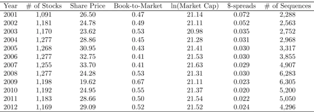
1.1 Year-by-year summary statistics of the final sample. Closing share prices,

book-to-market ratios, and log of market capitalizations are reported as the medians of their monthly values. $-spreads are the median time-weighted dollar bid-ask spread at the NBBO. The last column reports the median number of trade sequences (each with an aggregate value of at leastVj,t) in a year across stocks. . . 18

1.2 Trading costs and instrumented trading activity. For each stock-year observation, the absolute return realized over a trade sequence is regressed on the corresponding in-strumented trading activity percentile. The empirical distributions of these point estimates within each size decile are used to draw statistical inference. The sampling distribution is

assumed to follow a studenttdistribution (panel A). Observations are pooled across stocks

within a size decile. Absolute return is regressed on the corresponding instrumented trading activity percentile; partial regression outputs are reported (panel B). The point estimates

give the amount by which trading costs change asinstrumentedtrading activity rises from

1st percentile to the 99th. Results are reported for 2001–2012, and subperiods 2001–2006

and 2007–2012 . . . 37

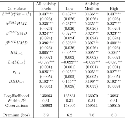
1.3 Augmented CAPM including trade-time liquidity measure. Estimation

re-sults for (1.6) using the trimmed sample, where the error term allows for stock fixed effects. Standard errors are clustered at the stock level. Month dummies capture any common variation in excess returns. β(rmkt

t −r

f

t) is the product of a firm’s market

beta and excess monthly return based on monthly holding period returns from CRSP and 1-month treasury bills. BMt−1 is the previous period’s Book-to-Market ratio. Ln(Mt−1) is the natural logarithm of the firm’s market capitalization at the end

of previous month. BBDt−1 is the previous month’s trade-time illiquidity measure

based on θ= 0.04. Symbols ∗, ∗∗, and∗∗∗ denote significance at 10%, 5%, and 1% levels, respectively. Robust standard errors are reported in parentheses. Premium is the product of theBBDcoefficient and the median value ofBBD. . . 43

(12)

1.4 Augmented CAPM using standard illiquidity measures. The table reports panel estimates of (1.6) using AM L, AM H, P SP, and DSP. Month dummies capture common variation caused by market condition changes, i.e., by common variation in excess returns over time. Standard errors are clustered at the stock level. Stock fixed effects capture any fixed heteroskedasticity. Observations in the top 1% tail of the relevant illiquidity measure are excluded. Symbols ∗, ∗∗, and∗∗∗ denote significance at 10%, 5%, and 1% levels, respectively. . . 47 1.5 Augmented CAPM estimates for orthogonal decompositions. The table reports

panel estimation results for (1.6) using the full sample. Standard errors are clustered at the stock level. Stock fixed effects capture any fixed heteroskedasticity. Month dummies capture any common variation caused by market condition changes. We separately present results

that contrast BBDagainst each alternative measureAM L,AM H, andP SP. Durations

are generated based on θ = 0.04. Observations in the upper 1% tail of either BBD or

F ∈ {AM L, AM H, P SP}in a month are excluded. Robust standard errors are reported

in parentheses. Symbols ∗,∗∗, and∗∗∗ denote significance at the 10%, 5%, and 1% level,

respectively. . . 48

1.6 Subsample estimation of augmented CAPM with different liquidity measures.

Panel estimation results of (1.6) for three subsamples: April 2001–Dec 2007, Jan 2008–Dec 2009, and Jan 2010–Dec 2012. Standard errors are clustered at the stock level. Stock fixed effects are introduced to capture any fixed heteroskedasticity. Month dummies are included to capture any common variation caused by market condition changes. The first column

for a given sub-sample present results for ourBBDmeasure based onθ= 0.04 computed

over all trade sequences. The other three columns of a panel present estimation results for

the standard liquidity measures, AM L,AM H, andP SP. Observations in the upper 1%

tail of the relevant liquidity measure are excluded. Robust standard errors are reported in

parentheses. The symbols ∗, ∗∗, and ∗∗∗ denote significance at 10%, 5%, and 1% levels,

respectively. . . 49

2.1 Sample mean and confidence intervals of correlation parameters, isolating in-creases from reductions in stock-specific market activity. Model 2.5 is estimated

each year, stock by stock, on subsamples representing increases in activity (yielding ˜ρjy)

and decreases in activity (yielding ˆρjy). Sample means and 99% confidence intervals of

correlation parameters ( ˜ρin panel A and ˆρin panel B) are reported by size group in periods

2001–2006 and 2007–2012. The cumulative trade value over each trade sequence is$80,000

plus 0.025% of market-capitalization. . . 73

2.2 Sample mean and confidence intervals of correlation parameters, isolating in-creases from reductions in stock-specific market activity by year. Model 2.5 is estimated each year, stock by stock, on subsamples representing increases in activity

(yield-ing ˜ρjy) and decreases in activity (yielding ˆρjy). Sample means and 99% confidence intervals

of correlation parameters ( ˜ρand ˆρ) are reported by year. The cumulative trade value over

(13)

2.3 Sample means and confidence intervals of correlation parameter estimates, iso-lating increases from reductions in activity by starting stock-specific market activity level. Model 2.5 is estimated year-by-year, stock-by-stock, on subsamples

repre-senting increases in activity (yielding ˜ρjy) and decreases in activity (yielding ˆρjy). Sample

means and 99% confidence intervals of the correlation parameter are reported by starting

activity group. Panel A reports the sample mean confidence intervals correlation parame-ters given no restrictions on activity changes. Panel B reports sample means and confidence

intervals for activity changes that are less than twenty activity percentiles. . . 81

2.4 Sample means and confidence intervals of correlation parameter estimates, iso-lating increases from reductions in activity by concluding trading activity level.

Model 2.5 is estimated year-by-year, stock-by-stock, for each activity quintile, on

subsam-ples representing increases in activity (yielding ˜ρjy) and decreases in activity (yielding ˆρjy).

Sample means and 99% confidence intervals of the correlation parameter are reported by

concludingactivity group. Panel A reports the sample mean confidence intervals correlation parameters given no restrictions on activity changes. Panel B reports sample means and

confidence intervals for activity changes that are less than twenty activity percentiles. . . . 84

2.5 Conditional likelihood of return persistence as a function of stock-specific mar-ket activity level and the size of activity change. For each stock-year, pairs of successive trade sequences are grouped into quintiles of starting/concluding activity. For each activity quintile, observations are classified into groups of changes in activity percentile: percentile changes are categorized into (−20,−10), (−10,0), (0,10), and (10,20) to reflect large decreases, small decreases, small increases, and large increases, respectively. Relative frequencies of successive returns of same sign are computed at the stock level. Reported conditional likelihoods reflect averages of such relative frequencies across stocks and time

by category. (∗) symbolizes the categories whose results are subject to potential selection

biases. . . 85

2.6 Sample means and confidence intervals of correlation parameter estimates, iso-lating increases from reductions in activity at highest and lowest levels of signed trade imbalance by stock size decile. Model 2.5 is estimated year by year, stock by

stock, for the highest and lowest starting/concluding imbalance quintiles, on subsamples

representing increases in activity (yielding ˜ρjy) and decreases in activity (yielding ˆρjy).

Increases and decreases in activity that exceed twenty percentiles are excluded. Sample means and 99% confidence intervals of the correlation parameter are reported by stock size decile. Panel A (Panel B) reports the sample means and confidence intervals of correlation

parameters at different starting (concluding) signed trade imbalance levels . . . 90

2.7 Mean relative frequency of increases/decreases in trading activity at different time-of-day windows by size decile. For each stock year, pairs of successive trade se-quences are categorized by the start time of the second sequence into three time windows: early, 9:30:00AM–11:30:00AM; mid-day, 11:30:00AM–2:00:00PM; and late, 2:00:00PM–4:00:00PM. The relative frequencies of increases and decreases in activity are computed across time win-dows for each stock-year. Relative frequencies are averaged across stocks and years by size

(14)

2.8 Sample mean and 99% confidence intervals of of ρj,y estimates that distin-guish increases from decreases in activity at different time-of-day windows by stock size decile Model (2.5) is estimated year-by-year, stock-by-stock by time-of-day window: early, 9:30:00AM–11:30:00AM; mid-time-of-day, 11:30:00AM–2:00:00PM; and late, 2:00:00PM–4:00:00PM. Model 2.5 is estimated year-by-year, stock-by-stock, for each time

window, on subsamples representing decreases in activity (yielding ˆρjy, Panel A) and

in-creases in activity (yielding ˜ρjy, Panel B). Activity changes are less then twenty percentiles.

Stocks are sorted by their market-capitalizations at the beginning of each year into size

deciles. Sample means and confidence intervals are computed by stock size decile. . . 99

2.9 Sample mean and 99% confidence intervals of of ρj,y estimates that distin-guish increases from decreases in activity at different time-of-day windows over

time Model (2.5) is estimated year-by-year, stock-by-stock by time-of-day window: early,

9:30:00AM–11:30:00AM; mid-day, 11:30:00AM–2:00:00PM; and late, 2:00:00PM–4:00:00PM. Model 2.5 is estimated year-by-year, stock-by-stock, for each time window, on subsamples

representing decreases in activity (yielding ˆρjy, Panel A) and increases in activity (yielding

˜

ρjy, Panel B). Sample means and confidence intervals are computed year-by-year. . . 102

3.1 Overview of transaction sequence duration: The median time duration of each stock’s transaction sequences is computed annually. Each year, stocks are grouped into size deciles based on market-capitalizations at the end of the previous year; size decile 1 contains stocks with smallest market-caps and size decile 10 contains those with largest. The second column of the table reports the cross-stock averages of stock-specific median durations, the third column reports the inter-quartile range of stock-specific median durations, and the last

column reports the cross-stock mean annual number of transaction sequences. . . 123

3.2 Number of insignificant estimates: WACD(2,2)s are fitted on a stock-year basis.

Re-ported are the number of cases where a particular parameter in an ACD fit isinsignificant

at 5% level. Durations measure the time it takes for a sequence of transactions worth

$80,000 plus 0.025% of market capitalization. Durations are adjusted for diurnal patterns

and overnight regime changes according to 3.4. . . 126

3.3 Predictability of duration and standardized duration series: yjt=π0j+

P20 i=2π j iI n jt+

ujt is estimated using the stock-year specific series if ˜xjtandjt. Mean point estimates and

mean t-statistics of{π2. . . π20}for the two series ˜xjt andjt are reported. The last row of

(15)

A.1 Signed trade imbalances versus trading activity and instrumented trading ac-tivity. For each stock-year observation, the absolute return realized over a trade sequence is regressed on the corresponding activity percentile (Panel A) or instrumented activity percentile (Panel B). The empirical distributions of these point estimates within each size decile are employed to draw statistical inference. The sampling distribution is assumed to

follow a student t distribution (“Stock level estimates”). Observations are pooled across

stocks within a size decile. Absolute return is regressed on the corresponding activity per-centile; partial regression outputs are reported (“Size group level estimates”). The point

estimates reflect the amount by which trade imbalances change as activity (instrumented

activity) rises from lowest to highest percentile. . . 144

A.2 Illiquidity coefficients in the two sub-periods, after orthogonal decomposition.

The table reports panel estimation partial results of (1.6) for two subsamples, April 2001– Dec 2006 and Jan 2007–Dec 2012. Standard errors are clustered at the stock level. Stock fixed effects capture any fixed heteroskedasticity. Month dummies capture common

varia-tion caused by market condivaria-tion changes. The coefficients of ztF−1 and ˜z

F

t−1 are reported,

the version ofBBDbased on all trade sequences is contrasted against the three standard

liquidity measures. Observations in the upper 1% tail of the relevant liquidity measures are

excluded. Robust standard errors are reported in parentheses. The symbols∗,∗∗, and∗∗∗

denote significance at 10%, 5%, and 1% levels, respectively. . . 149

B.1 Sample means and confidence intervals of correlation parameter estimates, iso-lating increases from reductions in trading activity in most and least active markets by stock size decile. Model 2.5 is estimated year by year, stock by stock, for the highest and lowest starting/concluding activity quintiles, on subsamples representing

increases in activity (yielding ˜ρjy) and decreases in activity (yielding ˆρjy). Increases and

decreases in activity that exceed twenty percentiles are excluded. Sample means and 99% confidence intervals of the correlation parameters are reported by stock size decile. Panel A (Panel B) reports the sample means and confidence intervals of the correlation parameters

(16)

List of Figures

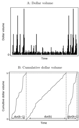
1.1 An illustration of how we measure the durations of trade sequences with

an aggregate value of at least Vj,t. . . 13

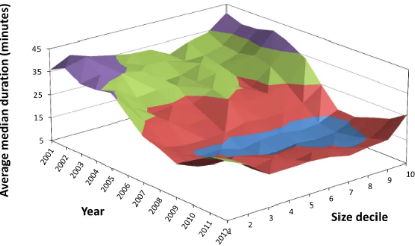
1.2 Trading activity by year and by firm size. Average median duration (in

min-utes) of a sequence of trades with a cumulative aggregate value of at least 0.04% of a firm’s market capitalization. Median durations are calculated on a stock-by-stock basis. The average is then computed for stocks in a size decile each year. Size decile 1 contains the smallest firms; decile 10 contains the largest. . . 19

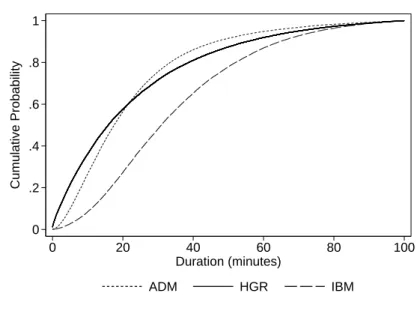
1.3 Distribution of durations of trade sequences for representative stocks.

Cu-mulative distribution functions of durations (in minutes) for International Business Machines (IBM), Archer Daniels Midland (ADM), and Hanger (HGR) from Jan-uary 1, 2001 to December 31, 2012. Durations are based on the elapsed time for a sequence of trades with a cumulative aggregate value of at least 0.04% of the firm’s market capitalization. . . 20

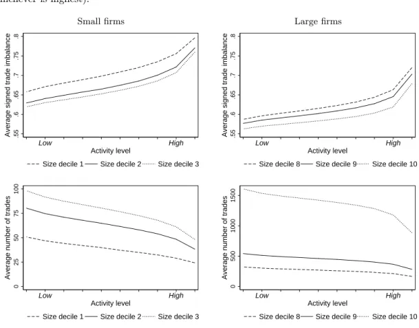
1.4 Average signed dollar-volume and average number of trades by trading

activity level. Average signed trade imbalance and average number of trades for

trade sequences with cumulative value of 0.04% of market capitalization in 2001–2012 versus activity level for the three deciles of smallest and largest stocks. Reported average signed trade imbalance and average number of trades are, respectively, the average of firm-specific annual mean estimated signed trade imbalance and number of trades (realized over trade sequences), computed at a trading activity level. Firm-specific means at a given trading activity level are averaged over all firms in a size decile, over the entire sample period. . . 21

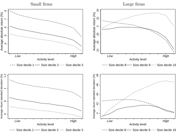
1.5 Average absolute return and return volatility by duration group. Market

impacts ofθ= 0.04% of market capitalization in 2001–2012 versus activity level for the three deciles of smallest and largest stocks. The reported average price impact is the average of firm-specific monthly means of absolute returns (realized over trade sequences), computed per duration group. Reported average return volatility is the average of firm-specific monthly standard deviations of returns (realized over trade sequences), computed per duration group. The averages of means and standard deviations are taken over all firms in a given size decile, over the entire sample period by activity level. . . 24

(17)

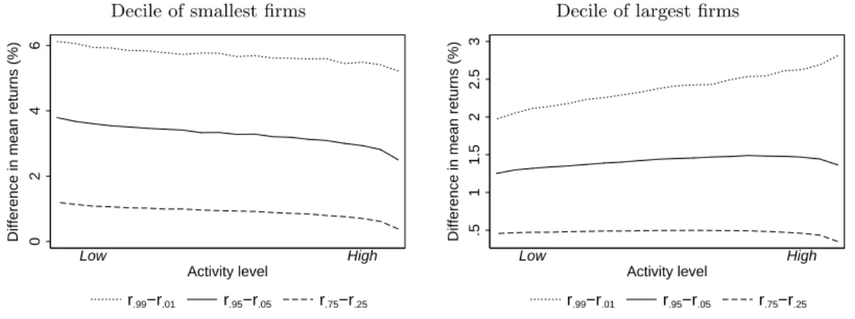
1.6 Estimated interpercentile ranges for realized returns by duration group. Plot of the interpercentile ranges of the distribution of realized returns for different activity levels. The percentile statistics of returns (realized over trade sequences) are first computed stock-by-stock, annually, for each duration group, and then aver-aged across stocks/years. Finally, the differences between selected average percentile statistics (r.99−r.01, r.95−r.05, andr.75−r.25) are computed by activity group.

Durations are based onθ= 0.04. . . 25

1.7 Empirical distribution of linear correlations and log-polynomialF-statistics

by size decile. In the top graphs, for each stock-year observation, we find the the

correlation between current duration and lagged number of trades. The kernel den-sity of these correlation coefficients is estimated by size groups. In the bottom graphs, for each stock-year observation, the current log duration is regressed on a second-order polynomial of the lagged number of trades and the corresponding F-statistic is obtained. We then estimate, by size groups, the kernel density for the empirical distributions of theF-statistics. The vertical dashed lines indicateF-statistics of 10. Values exceeding 500 are omitted for visual clarity. . . 30

1.8 Average absolute return by predicted activity group. Average absolute

re-turn of 0.04% of market-cap in 2001–2012 versus predicted trading activity for the deciles of smaller and larger stocks. The reported average absolute return is the average of firm-specific annual mean absolute return (realized over trade sequences), computed per predicted activity group. The average of means is taken across all firms in a given size decile, over the entire sample period by predicted activity level. Average absolute return versus activity is also displayed to highlight differences. Stock-year observations with first stage regression F-statistics below 10 are dropped. 32

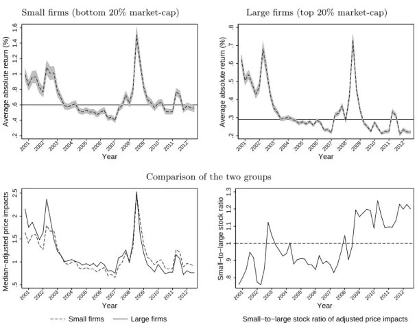
1.9 Temporal changes in average price impacts for small and large firms.

Stock-specific mean price impacts of 0.04% market-capitalization are computed quarterly. Then averages of these means are calculated quarterly across stocks in a market-cap

quintile. Average price impacts and the corresponding 99% confidence intervals are

presented for small (bottom 20% market-cap) and large (top 20% market-cap) stocks (top row)—the horizontal lines give medians of average price impacts are computed over the entire sample. The time series of price impacts normed by these sample medians are compared in the bottom row both in absolute and relative terms. . . 38

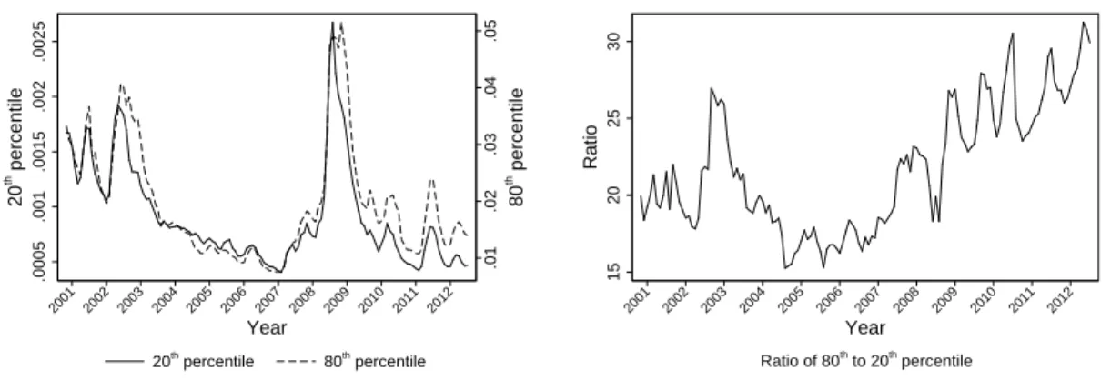
1.10 Temporal changes in levels and the ratio of the 20th _{and the 80}th

per-centiles of BBD. BBDis constructed based on all trade sequences. The 20th_and

the 80th_{percentiles of}_BBD _{are determined on a monthly basis. The ratio reflects}

the 80th_{percentile divided by the 20}th_{percentile every month. . . .} ₄₀

1.11 Monthly median values of different illiquidity measures over time. The

BBD measure (based on θ = 0.04) is calculated using observations from all trade sequences. Also shown is the high frequency Amihud measure (AM H), the low frequency Amihud measure (AM L) and percentage bid-ask spreads (P SP). . . 45

(18)

2.2 Time duration of trade sequences by year and by firm size. The figure reports the average median duration (in minutes) of a sequence of trades with a cumulative aggregate

value of at least$80,000 plus 0.04% of a firm’s market capitalization. The median duration

is first calculated on a stock-by-stock basis, and then the average is taken across stocks within a size decile in a year. Size decile 1 contains the smallest firms; decile 10 contains

the largest. . . 66

2.3 Average return by activity group. Average return trade sequences with cumulative

value of$80.000 plus 0.025% of market capitalization in 2001–2012 versus activity level by

stock size categories. Reported average return is the average of firm-specific annual mean returns (realized over trade sequences), computed per activity group. The average of means

is taken across all firms in a given size decile, over the entire sample period by activity group. 67

2.4 Empirical distributions of correlation parameter estimates and the correspond-ing t-statistics, isolatcorrespond-ing increases from decreases in stock-specific market ac-tivity. Model 2.5 is estimated year-by-year, stock-by-stock, on subsamples representing

increases in activity (yielding ˜ρjy) and decreases in activity (yielding ˆρjy). The top row

re-ports the empirical distributions of ˜ρand ˆρ, separately for stocks falling in the bottom 30%,

middle 40%, and top 30% of beginning-of-the-year market-capitalizations, for the periods 2001–2006 and 2007–2012. The bottom row exhibits the corresponding t-statistics with vertical lines standing for the 95% critical values for relevant one-sided significance tests.

The cumulative trade value over each trade sequence is $80,000 plus 0.025% of

market-capitalization. . . 70

2.5 Empirical distributions of correlation parameter estimates for signed past re-turns, isolating increases from decreases in stock-specific market activity. I estimate model 2.5 each year, stock by stock, on subsamples representing increases in

activ-ity (yielding ˜ρjy) and decreases in activity (yielding ˆρjy), conditioning on the sign of return

realized over the first trade sequence, rjy(k−1). The cumulative trade value over each

trade sequence is$80,000 plus 0.025% of market-capitalization. . . 74

2.6 Empirical distributions correlation parameter estimates that isolate increases from reductions in activity by starting stock-specific market activity level.

Model 2.5 is estimated each year stock by stock, for eachstartingactivity quintile, on

sub-samples representing increases in activity (yielding ˜ρjy) and decreases in activity (yielding

ˆ

ρjy). The top row displays the empirical kernel densities of estimated correlations with no

restrictions on activity changes. The bottom row reports similar densities whose estimates

are based on activity changes that are less than twenty activity percentiles. . . 80

2.7 Empirical distributions correlation parameter estimates that isolate increases from reductions in activity by concluding stock-specific market activity level.

Model 2.5 is estimated year-by-year, stock-by-stock, for each concluding activity quintile,

on subsamples representing increases in activity (yielding ˜ρjy) and decreases in activity

(yielding ˆρjy). The top row displays the empirical kernel densities of estimated correlation

estimates with no restrictions on activity changes. The bottom row reports similar densities

(19)

2.8 Empirical distributions correlation parameter estimates that isolate decreases in activity by starting/concluding signed trade imbalance level for stock size groups. Model (2.5) is estimated year-by-year, stock-by-stock, controlling for conclud-ing/starting imbalance quintiles for the subsample of trade sequences associated with a

decrease in activity (yielding ˆρjy). Decreases in activity that exceed twenty percentiles are

excluded. The top (bottom) row reports the empirical density estimates at the highest and

lowest starting (concluding) signed trade imbalances. . . 88

2.9 Empirical distributions of correlation parameter estimates that isolate increases in activity by starting/concluding signed trade imbalance level for stock size groups. Model (2.5) is estimated year-by-year, stock-by-stock, controlling for conclud-ing/starting imbalance quintiles for the subsample of trade sequences associated with a

increase in activity (yielding ˆρjy). Increases in activity that exceed twenty percentiles are

excluded. The top (bottom) row reports the empirical density estimates at highest and

lowest starting (concluding) signed trade imbalance. . . 89

2.10 Sensitivity of current signed trade imbalance to past changes in activity by concluding stock-specific market activity level. The sample is decomposed by year,

size decile, and concludingactivity group—observations are pooled across different stocks.

Within each category, signed trade imbalance is regressed on the past change in activity percentile, inversely weighting observations on each stock by its number of trade sequences that year. The point estimates and the associated t-statistics are reported by activity groups and sub-periods (top row). Similar estimates are obtained, isolating samples of increases

and decreases in trading activity (bottom row). . . 94

2.11 Sensitivity of current price impact to past changes in activity by concluding stock-specific market activity level. The sample is decomposed by year, size decile, and concluding activity group—observations are pooled across different stocks. Within each category, price impact is regressed on the past change in activity percentile, inversely weighting observations on each stock by its number of trade sequences that year. The point estimates and the associated t-statistics are reported by activity groups and sub-periods (top row). Similar estimates are obtained, isolating samples of increases and decreases in

tradting activity (bottom row). . . 95

2.12 Empirical distributions of ρj,y estimates that distinguish increases from de-creases in activity at different time-of-day windows by stock size group. Model (2.5) is estimated year-byyear, stock-by-stock by time-of-day window: early, 9:30:00AM–11:30:00AM; mid-day, 11:30:00AM–2:00:00PM; and late, 2:00:00PM–4:00:00PM. Model 2.5 is estimated year-by-year, stock-by-stock, for each activity quintile, on subsamples representing increases

in activity (yielding ˜ρjy, top row) and decreases in activity (yielding ˆρjy, bottom row).

Activity changes are less then twenty percentiles. Stocks are sorted by their

market-capitalizations at the beginning of each year into bottom 30%, middle 40%, and top 30%

(20)

2.13 The temporal evolution of the commonality in the return corelations associated with increases and decreases in stock-specific market activity. Every quarter, I estimate the correlation structure of returns realized over two successive trade sequences for the sample of increases in activity and for the sample of reductions in activity, stock-by-stock. I then estimate the cross-stock correlations of these two correlation parameters

quarterly. . . 104

2.14 The temporal evolution of mean change in proportion of buyer-initiated trad-ing when stock-specific market activity falls by signed past returns.Samples of successive trade sequence pairs that represent reductions in activity are decomposed by signing the return realized over the first trade sequence of each pair (past return). To avoid selection bias, the reduction in activity must be smaller than twenty activity percentiles. For each stock, the mean change in the proportion of buyer-initiated trades, associated with a decline in activity after signed returns, is computed annually. Averages of those means are taken across stocks of a size group (bottm 30%, middle 40%, and top 30% of

market-capitalizations at the beginning pf each year) year-by-year. . . 106

2.15 The relation between concluding stock-specific market activity level and the change in the proportion of buyer-initiated trades as trading activity declines.

Samples of successive trade sequence pairs that represent reductions in activity are de-composed by signing the return realized over the first trade sequence of each pair (past return). To avoid selection bias, the reduction in activity must be smaller than twenty activity percentiles. For each stock, the mean change in the proportion of buyer-initiated trades, associated with a decline in activity after signed returns, is computed by activity decile, annually. Averages of those means are taken across stocks of a size group (bottm 30%, middle 40%, and top 30% of market-capitalizations at the beginning pf each year) and over time within the periods 2001–2006 and 2007–2012 by activity decile. Solid and dashed

curves signify positive (negative) past returns, respectively. . . 108

2.16 The relation between concluding stock-specific market activity level and the change in the proportion of buyer-initiated trades as trading activity declines by time of day in 2007–2012. Samples of successive trade sequence pairs that represent reductions in activity are decomposed by signing the return realized over the first trade sequence of each pair (past return). To avoid selection bias, the reduction in activity must be less than twenty activity percentiles. For each stock, the mean change in the proportion of buyer-initiated trades, associated with a decline in activity after signed returns, is computed

by activity decileandtime of day, annually. Averages of those means are taken across stocks

in a size group and over time within the period 2007–2012 by activity decile.. . . 110

3.1 Calculations of successive transaction sequences of a given stock. . . 121

3.2 Empirical distributions of parameter estimates: WACD(2,2)s are fitted on a stock-year basis. The histograms reflect the empirical distributions of stock-stock-year-specific estimates

of parameters {αj1, α j 2, β j 1, β j 2, ω j

, γj}. Durations measure the time it takes for a sequence

of transactions worth$80,000 plus 0.025% of market capitalization. Durations are adjusted

(21)

3.3 Pair-wise correlations of parameters: WACD(2,2)s are fitted on a stock-year basis. The scatter plots reflect the pair-wise associations between stock-year-specific estimates of

parameters {αj₁, αj₂, β₁j, β₂j, ωj, γj}. Durations measure the time it takes for a sequence of

transactions worth $80,000 plus 0.025% of market capitalization. Durations are adjusted

for diurnal patterns and overnight regime changes according to 3.4.. . . 129

3.4 Shape parameter estimates and log-number of durations against stock size:

Stock-year specific shape parameter estimates γjs and log-number of durations are

plot-ted against stock size percentile. Size percentiles reflect annual normalized rank statis-tics that sort stocks from smallest to largest by market-capitalization each year—market-capitalizations are measured at the end of the previous year. Durations measure the time

it takes for a sequence of transactions worth$80,000 plus 0.025% of market capitalization.. 131

3.5 Empirical distributions of AR(2) coefficients and their corresponding t-statistics:

yjt=δj0+δ

j

1yjt−1+δj2yjt−2+ujtis estimated using the series of ˜xjtandjtfor each stock-year

set of observations. The empirical distributions of the corresponding parameter estimates and t-statistics for the two series types are contrasted. Vertical short-dashed lines in the bottom row represent two-sided critical values at 0.1% significance level. Durations

mea-sure the time it takes for a sequence of transactions worth $80,000 plus 0.025% of market

capitalization. . . 133

3.6 Point estimates and t-statistics of mean hazard errors: WACD(2,2)s are fitted on a stock-year basis. Using stock-year-specific estimates, hazard errors (ratios of

empirical-to-predicted hazard) are computed for eachjt. Observations on each stock-year are sorted

into twenty equally-sized groups of standardized duration (jt), and mean hazard errors are

computed by standardized duration group per stock-year set of observations. The top row presents the averages of mean hazard errors at different levels of standardized duration; the bottom row reports the corresponding t-statistics for a null of average error equal to unity (the two horizontal lines stand for critical values at 0.1% significance level). Averages and t-statistics are calculated across stocks and years, controlling for stock size decile. Size deciles are formed at the beginning of each year by sorting stocks into ten equally-sized

groups of market-capitalizations at the end of the previous year. . . 135

A.1 Average signed trade imbalances versus predicted trading activity. Average

signed trade imbalances of trade sequences versus predicted trading activity for the deciles of smaller and larger stocks. The reported average signed-dollar volume is the average of firm-specific annual mean dollar-weighted proportion of buy- (sell-) oriented trades (realized over trade sequences(sell-), computed per predicted activity group. The average of means is taken across all firms in a given size decile, over the entire sample period by predicted activity group. Average signed trade imbalances versus trading activity is displayed to highlight differences. Stock-year observations with first stage regression F-statistics below 10 are dropped. . . 143

(22)

A.2 Average daily return volatility by activity group. Average return volatility of 0.04% of market capitalization in 2001–2012 versus activity level for the three deciles of smallest and largest stocks. The reported average daily return volatility is the average of firm-specific annually computed daily standard deviations of returns

SD

i (y, j), computed per duration group. The average of daily standard deviations is

taken across all firms in a given size decile, over the entire sample period, by activity level. . . 145

A.3 Empirical cumulative density functions of duration by size decile.

Dura-tions are computed based onθ= 0.04 and their CDFs are presented for two subsets of large and small stocks, over the entire period (2001–2012), and the early (2001-2006) and later (2007–2012) sub-periods. To calculate the CDF of durations for stockj in year y, every month, we first sort durations into 20 buckets, each containing 5% of observations. Then we pool buckets across different months. The median of these durations corresponds to the quantile statistic falling at the midpoint of that dura-tion bucket. For example, the median in the pooled bucket of shortest 5% estimates quantile statistic 2.5%; that for next bucket estimates quantile statistic 7.5%; etc. For each duration bucket, we average the stock-specific quantile statistic estimates over years and stocks in size decile x. Plotting these averages against their rele-vant percentile points, for each size portfolio, yields the empirical CDF of durations conditional on firm size. . . 150

A.4 Average absolute return, return volatility, and average number of trades

versus signed trade imbalance. Average absolute return, average return

volatil-ity, and mean number of trades for trade sequences versus signed trade imbalance for deciles of smaller and larger stocks. We first sort trade sequences into ten equally-sized groups of percent signed trades, every month. The reported averages are the sample averages of firm-specific annually-computed mean absolute return, return standard deviation, and mean realized depth (all assessed over sequences), computed per signed trade imbalance decile. The averages of means are taken across all firms in a given size decile, over the entire sample period by signed trade imbalance level. 151

B.1 Empirical distributions correlation parameter estimates that isolate decreases in activity by starting/concluding stock-specific market activity level for stock size groups. Every year, model (2.5) is estimated stock by stock, controlling for conclud-ing/starting trading activity quintiles. Estimates are obtained using the sample of trade

sequences that are associated with a decrease in activity (yielding ˆρjy). Decreases in activity

that exceed twenty percentiles are excluded. The top (bottom) row reports the empirical

density estimates at highest and lowest starting (concluding) activity levels. . . 153

B.2 Empirical distributions correlation parameter estimates that isolate increases in activity by starting/concluding stock-specific market activity level for stock size groups. Every year, model (2.5) is estimated stock by stock, controlling for conclud-ing/starting trading activity quintiles. Estimates are obtained using the sample of trade

sequences that are associated with an increase in activity (yielding ˜ρjy). Increases in

activ-ity that exceed twenty percentiles are excluded. The top (bottom) row reports the empirical

(23)

B.3 Sensitivity of current signed trade imbalance to past changes in activity by concluding stock-specific market activity level. The sample is decomposed by year,

size decile, and starting activity group—observations are pooled across different stocks.

Within each category, signed trade imbalance is regressed on the past change in activity percentile, inversely weighting observations on each stock by its number of trade sequences that year. The point estimates and the associated t-statistics are reported by activity groups and sub-periods (first row). Similar estimates are obtained, isolating samples of increases

and decreases in trading activity (second row). . . 157

B.4 Sensitivity of current price impact to past changes in activity by concluding stock-specific market activity level. The sample is decomposed by year, size decile, and starting activity group—observations are pooled across different stocks. Within each category, signed trade imbalance is regressed on the past change in activity percentile, inversely weighting observations on each stock by its number of trade sequences that year. The point estimates and the associated t-statistics are reported by activity groups and sub-periods (first row). Similar estimates are obtained, isolating samples of increases and

(24)

Chapter 1

Trading costs and priced illiquidity

in high frequency trading markets

I

Introduction

Prior to 1997, stock prices were quoted in eighths, and this tick size drove trading costs and limit order book depth. Today, the typical tick size is a penny, and depth near inside quotes has collapsed. The primary providers of market-making services are now algorithmic and high frequency traders (HFT henceforth) who submit many thousands of small, fleeting orders each trading day. As a result, average trade sizes, inside bid-ask spreads and depth are tiny.

To establish and unwind positions, institutional investors now employ specialized brokers who use sophisticated algorithms to split intended trading positions into many small orders that are dynamically submitted over time and across trading venues. This makes institutional “child orders” temporally dependent, a phenomena that HFT can profitably exploit, further raising institutional trading costs. Individual transactions and the corresponding price changes largely reflect execution processes, not institutional trading decisions. The price change associated with each small individual trade trivially contributes to trading costs, implying that traditional measures of trading costs and liquidity no longer describe concerns of institutional investors. Rather, institutional investors care about the cumulative price impacts of these trades that together comprise their larger intended trade positions.

(25)

The key contributions of our paper are to measure these trading costs, how they vary with the level of market activity and firm characteristics, and to show how these trading costs explain the cross-section of expected returns in asset pricing models. We identify the primitive economic forces underlying the variations in trading costs, trade sizes and signed trade imbalances at different trading activity levels, teasing out implications for theorists seeking to understand today’s markets. We also identify how the divergence of trading costs in the cross-section of stocks translates to greater liquidity premia post RegNMS.

We first develop a stock-specific measure of trading activity that serves as a tool to isolate different trading activity conditions. We then use it to measure how trading costs vary with the level of trading activity, firm size and time. Our findings indicate that, on average, endogenous consumption of liquidity, not information arrival, is the primary driver of trading activity and the associated price impacts. This inference highlights the importance of identifyingwhen to begin to establish or unwind a position. We employ a simple instrument to control for this endogeneity, and show how an institutional investor can predict future stock-specific trading activity levels, and thereby optimally time trades.

We then establish that, over time, theshapesof trading cost-trading activity level relationships have become more similar across stocks—in recent years, as trading activity rises, trading costs decline in similar ways for most stocks—suggesting that markets of different stocks became more homogeneous in an important way. In other ways, however, the RegNMS and advent of algorithmic trading seem to have increased cross-stock heterogeneity: we find that although the trading costs of larger and more liquid stocks have fallen in recent years, those of smaller and less liquid stocks have not. Finally, we establish that this divergence in trading costs translates into post-financial crisis illiquidity premia that exceed pre-crisis levels.

(26)

O’Hara (2015) highlights the ways in which changes in the market make individual trades min-imally relevant for existing microstructure models. Any measure of stock-specific trading activity must aggregate sufficiently to control for the temporal dependence of trades, but not by so much that one aggregates over very different market conditions. Aggregation is also necessary to deal with issues with available data sets.1 The question becomes: how to aggregate? There are two popular approaches.

Amihud (2002) aggregates volume over a trading day to construct his price impact measure. One could modify his approach by aggregating over shorter (e.g., twenty minute) time intervals within a trading day, where greater volumes indicate greater activity. For our purposes, this approach does not work. Such aggregation gives rise to massive variation in trading volumes across time intervals. As a result, intervals with very low volume deliver noisy measures of market metrics such as returns, and represent far lower volumes than would be relevant for institutional investors. In addition, intervals with volume spikes aggregate over different market conditions. Furthermore, aggregating in this way means that relationships between price impacts and trading volumes conflate both activity and volume: it is unclear whether a positive relationship between price impacts and volume in a fixed time interval is due to higher activity, or to activity being linked to volume, which in turn is positively correlated with price volatility (Andersen and Bondarenko (2014)).

Easley et al. (2012) instead divide trading volume on each day into a fixed number ofequally-large

volume bundles (e.g., 50). Within a trading day, bundles that span longer time periods indicate lower activity. For our purposes, this approach also does not work: it leads to huge variation

1 _{O’Hara et al (2012) highlight that monthly TAQ data misses odd-lots that, on average, account for only 7% of}

trading volume, but 35% of price discovery. Braccini (2014) reports that 25% of trades coincide given millisecond time scales, which makes analysis of time series properties of trades challenging. Murvayev and Picard (2014) highlight issues of mechanical trade clusters. Holden and Jacobsen (2013) documents shortcomings of monthly TAQ relative to daily TAQ.

(27)

from one day to the next in volume bundle sizes, a variation that is compounded by the exploding trading volumes in recent years. Issues arise when trying to aggregate across days or over time for estimation purposes, because a low level of activity on one day is not comparable with a low level on another day.

To circumvent these issues, we develop a novel aggregation method that groups consecutive transactions together into atrade sequencewith a fixed cumulative target dollar value (e.g., 0.04% of a firm’s market capitalization). Once a stock’s target dollar value is reached, we start over, grouping the next set of consecutive trades until their cumulative dollar value reaches its target value, continuing in this way iteratively over a year. We measure trading activity by the time it takes for a trade sequence to reach its target dollar value—shorterdurationsindicate more active markets. Controlling for the dollar value of a sequence preserves two key features: (1) it delivers comparable fundamentals measured over different trade sequences of a stock; (2) it lets us isolate

the effects of activity from those of trading volume. By setting target dollar values neither too

large nor too small, we address concerns about (a) aggregating over multiple activity levels due to excessively large targets, (b) mis-attributing variation in activity due to excessively small targets, and (c) the impact of missing odd-lots; and it delivers trade volumes of interest to institutional investors, objects that are economically and empirically tractable.

We first show that both trade size and signed trade imbalance rise with trading activity: on average, as the duration of a trade sequence for a stock shrinks, (1) fewer trades comprise the sequence and (2) trade becomes less balanced.2 _{Going from least to most active markets, signed}

trade imbalances rise by roughly 20%, and for small stocks, mean trade sizes double.

2_{We use the Lee and Ready (1991) algorithm to identify the share of value-weighted trades in a trade sequence}

(28)

It is not surprising that more active markets feature more aggressive trading. Classical models of speculation (Kyle (1985), Easley and O’Hara (1992), Glosten (1994)) predict precisely this: speculators with substantial private information will establish larger positions, submitting larger marketable orders that cause trading activity, signed trade imbalance, and trade sizes all to rise. But, a very different explanation presents itself. Liquidity provision may be state-varying—more depth may be available near inside quotes at some times than others. When the market is unusually liquid on one side, traders respond aggressively, submitting larger marketable orders that are filled at these “good” prices. As a result, the corresponding trade sequences have shorter durations, with fewer trades and less balanced signed trade. In contrast, with little depth, traders submit less aggressive orders (i.e., marketable orders that consume less liquidity), and submit more passive orders (i.e., limit orders that supply liquidity) to reduce price impacts.3 The result is lower trading activity, more balanced signed trade, and more trades comprising a trade sequence.

To distinguish between these two explanations, we look at price impacts. Models of speculation predict that more aggressive trading should lead to larger price impacts; but, if endogenous con-sumption of unusually high depth at “good” prices is the primary driver, price impacts should fall as activity rises. We measure price impacts in two ways: (1) the average absolute return over a trade sequence at a trading activity level; and (2) the average annual standard deviation of those returns. For small and mid-sized stocks, both price impact measuresfall sharplyas trading activ-ity rises—declines on the order of 40%. Thus, even though volatilactiv-ity is positively associated with volume and activity, the opposite relationship holds once one controls for volume. In contrast, for larger stocks, price impacts peak at intermediate activity levels, and, indeed, the standard deviation of returns is smallest when markets areleastactive.

3_{See Bloomfield et al. (2005), Goettler et al. (2005), Hollifield et al. (2004), Hollifield et al. (2006) or Easley et}

(29)

The uniformly negative relationship between price impacts and activity for small and mid-sized stocks indicates that varying endogenous consumption and provision of liquidity is the key driver of variation in trading activity and price impacts, not information. In contrast, fat tails of the return distribution in active markets of large stocks suggests that, in unusual times, information arrival drives some higher activity, but, in normal times, activity mostly reflects variation in liquidity.

Advice to investors who seek to minimize trading costs to “trade when markets are liquid at good prices” has modest value. Thus, we proceed to isolatestableandpredictableactivity–trading cost relationships: we examine how price impacts vary withpredictedtrading activity.

To control for information arrival and the endogeneity of order composition, we use the number of trades filling the previous trade sequence to instrument for the time duration of the current trade sequence. The insight underlying this instrument is that liquidity persists over time—present and past states of the order book are positively correlated. The endogenous composition of current orders, however, hinges only on the contemporaneous state of the order book, which strongly co-varies with current activity and price impacts. Effects of past order book states on current price impacts only transmit via the current state of the order book and the dollar volume in a trade sequence is large enough to minimize the temporal dependence associated with endogenous order composition. Intuitively, the endogenous responses quickly offset imbalances in liquidity—when liquidity is high, it is consumed, and when it is low, it is provided. Appropriate aggregation is crucial for this result, since at ultra-high frequency, it takes some time for “unusual” liquidity to be absorbed, as Hirschey (2013) shows.

We provide extensive evidence that our instrument choice is a good one, and that signed trade imbalances only rise weakly with predicted trade activity. In sharp contrast,verystable and uniform

(30)

trading costs–predicted trading activity relationships obtain across all firm sizes. Instrumenting flattens the price impact/activity relationship for small stocks by roughly 75%; but for larger stocks, the price impact/activity relationship not only becomes monotone, it becomessteeper. The uniform reduction in average price impacts (of a trade sequence) of five to eight basis points as predicted market conditions rise from least active to most active levels are meaningful from the perspective of an institutional investor.

We next investigate how trading costs evolved between 2001 and 2012 as U.S. equity markets were transforming. We first show that in more recent years the relationship between predicted trad-ing activity and tradtrad-ing costs became more similar across stocks—tradtrad-ing costs fall by comparable amounts as predicted trading activity rises. But, markets did not become uniformly more liquid:

levelsof price impacts ofmore liquid stocksfellpost crisis, but those ofless liquidstocksrose. As

such, the narrower bid-ask spreads of recent years are a misleading indicator of changes in trading costs. These findings lead us to explore their asset pricing implications.

To create a measure of individual stock liquidity that is appropriate for today’s markets we scale our price impact measure by the dollar amount traded. Our illiquidity measure, denotedBBD, is a rolling average of the per-dollar price impact of trading a fixed proportion of a stock’s market capitalization that controls for trading activity level. BBD is a trade-time analogue of Amihud’s (2002) temporal measure of liquidity that isolates the effects of trading activity from trading volume and controls for the variation in trading costs with activity.

Regardless of which trading activity levels are used to calculate BBD, it is priced in an aug-mented capital asset pricing model (CAPM), and indeed similar illiquidity premia obtain. We verify thatBBDbetter captures illiquidity considerations of investors than do standard illiquidity

(31)

measures—average percentage bid-ask spreads, Amihud’s per dollar price impact, and a high fre-quency version of Amihud’s measure constructed at hourly frequencies—especially, post RegNMS. To do this, given the high correlation in the measures, we employ the residuals from the regression of one measure on a second in the pricing regressions. TheBBDresidual is always priced, whereas the other residuals are not.

We then show that illiquid stocks become more illiquid post RegNMS, and that liquid stocks became more liquid. Splitting the sample into pre-crisis, crisis, and post-crisis periods reveals that despite far higher trading volumes associated with high-frequency trading, illiquidity premia post-crisis exceed pre-crisis levels. That is, increased cross-stock dispersion in trading costs and illiquidity translates to greater dispersion in expected excess returns.4

Our paper is organized as follows. We next discuss related research. Section II develops our trading activity measure. Section III shows how various fundamentals vary with activity. Section IV evaluates the illiquidity measures in an asset pricing model. Section V concludes. Chapter A explores calendar time relationships between volatility and stock-specific trading activity, and shows our results are robust to different error structure specifications.

A

Related Literature

Trade time and market dynamics. Mapping financial market dynamics onto trade-time space

is not a new idea. Dufour and Engle (2000) examine the duration between successive trades and show that price adjustments are faster when trading intensities are high (i.e., durations are short). They argue that high trade intensities reflect informed trading and conclude that these periods

4_{In contrast, Ben-Rephael et al. (2015) find lower liquidity premia in 2000-2011 than in earlier sub-periods between}

(32)

represent periods of market illiquidity. Engle and Russell (1998) and Engle (2000) develop related models of autoregressive conditional duration (ACD) that provide semi-parametric estimates of trade intensities based on trade arrival rates. ACD models are largely designed to estimate the expected cost and time to execute a single order, submitted within a short time frame, not the cost of a series of orders submitted over a longer window.

In modern markets, the information content of one trade is small; and consecutive trades may represent a single trading decision, where a larger order is crossed against multiple smaller orders in the book. To account for these features, Gouri´eroux et al. (1999) measure activity by the time it takes the market to execute an exogenous level of volume or dollar volume. They focus on the evolution of trading activity over the trading day on Paris Bourse for a single stock over 18 trading days, exploring the average time duration to unwind a fixed position at different times. They find activity peaks at times corresponding to the opening of the London Stock Exchange and NYSE. Easley et al. (2012) are similarly motivated to group consecutive trades across time according to the time required to trade an exogenous level of order flow. Within each group, they use the sign of price changes over one-minute periods to infer buyer-initiated versus seller-initiated trades, creating a measure of volume “toxicity”, VPIN, the high frequency analogue to their probability of informed trading (PIN) measure.5

Feldh¨utter (2012) develops the notion of an imputed roundtrip trade, based on the empirical feature that trades in corporate bonds often occur infrequently, but when they do trade, there are often several trades in a short period of time. He argues that these trades are likely linked and

5_{Our findings indicate a tension between concerns about using and consuming liquidity, and identification of}

probabilities of informed trade off of a zero-profit limit order pricing condition. If liquidity provision is competitive, traders should always consume liquidity—it isbecausemarkets are sometimes more liquid than others that a trader sometimes consumes and sometimes supplies liquidity (Andersen and Bondarenko (2014)). Based on execution algorithms of ITG, O’Hara (2015) provides evidence of order-splitting strategies that employ variable weights of aggressive and passive orders at different levels of institutional trade intensity.

(33)

should be considered together when measuring trading costs.

Relation between trading activity and liquidity. There has been a long debate about the

relation between activity and liquidity. Demsetz (1968) finds that more active stocks tended to be more liquid, and argues that more frequent trading is associated with low dealer costs. Lippman and McCall (1986) argue that active markets have a lower opportunity cost of searching and are thus more liquid. Jones (2002) and Fujimoto (2004) find no relation between liquidity measures and changes, or shocks, in turnover. Johnson (2008) develops a model in which volume is positively re-lated to liquidityrisk, rather than liquidity, and provides supporting evidence from U.S. government bond markets.

Liquidity Measures. Amihud and Mendelson (1986) show that when the standard tick size was

one-eighth, bid-ask spreads were priced and were a good measure of liquidity. Other quote-based liquidity measures include effective bid-ask spreads, Roll’s (1984) measure, and Hasbrouck’s Gibbs estimate.6 _{Lesmond et al. (1999) argue that periods of zero returns may represent an absence of}

informed trading, periods where informed trading costs are high.

Variants of Kyle’sλ(Kyle (1985)) have also been used as liquidity measures (see, e.g., Glosten and Harris (1988), Brennan and Subrahmanyam (1996), or P´astor and Stambaugh (2003)). Bern-hardt and Hughson (2002) estimate price impacts using a structural model whose equilibrium, unlike Kyle’s, explicitly incorporates orders that are not pooled.

Chordia et al. (2011), Angel et al. (2011), Kim and Murphy (2013), and others have questioned the accuracy and feasibility of many existing liquidity measures in a high frequency trading world with tiny spreads and little depth at the inside quote. Holden and Jacobsen (2014) document

6_{Effective bid-ask spreads measure the spread between the trade price and quote midpoint. Roll (1984) focuses}

on how the tick size induces negative autocorrelation in returns. Hasbrouck (2009) proposes a Bayesian platform to generate a Gibbs estimate of Roll’s effective trading cost indicator.

(34)

realized dollar spreads and share depth as low as 0.88¢ and 564 shares, respectively, for a sample of randomly selected stocks in 2008. Today, liquidity concerns do not revolve around avoiding minimum price ticks, so spreads do not capture liquidity from that perspective. Order-splitting makes consecutive trades dependent (Hasbrouck (2009), Easley et al. (2012)) and interpretations of estimates ofλheroic—especially since TAQ data omit odd-lots, which now account for 35% of price discovery. Moreover, high trading volumes result in few instances of zero returns (Mazza (2013)). Further, the increased use of hidden orders makes it difficult to measure depth directly. Deuskar and Johnson (2012) propose a measure of liquidity that uses information from the cumulative depth in the book, not just the inside quote. Unfortunately, using order book information is not feasible for most applications, and their measure is not designed to capture dynamic order splitting.

In light of these issues, liquidity measures based on volume, rather than orders have been developed. These aggregative measures are minimally affected by dynamic order-splitting and omission of odd-lots. The most widely used is Amihud’s (2002) measure, which is based on the ratio of absolute daily returns divided by daily dollar volume. This measure has been useful at explaining the cross-section of returns, and, indeed, in time series (Amihud (2002) and Jones (2002)). Goyenko et al. (2009) show that Amihud’s measure remains useful in the post-decimalization era. With increased high frequency trading, however, such low frequency measures may lose valuable information by aggregating across heterogeneous conditions.

Acharya and Pedersen (2005) incorporate a portfolio-level aggregate of Amihud’s measure in a market model and argue that premia can be explained by covariations of stock liquidity with market-wide return and this liquidity proxy. Akbas et al. (2011) extend Acharya and Pederson (2005) by adding a measure of idiosyncratic liquidity volatility. These papers are related to research on the commonality of market-wide liquidity (Chordia et al. (2000), Sadka (2006)). Our focus is

(35)

on illiquidity as a stock characteristic, as in Ben-Rephael et al. (2014).

II

Measuring Activity

To start, we define a trade sequence and explain how we use the time duration of a trade sequence to measure stock-specific trading activity. Each year, we number trades in stock j se-quentially, using indexnj. For tradenj, we useτj(nj),Qj(nj) and Pj(nj) to denote respectively,

(i) its time measured in seconds from the beginning of the year, (ii) its size (in shares), and (iii) its price. We construct our activity measure by calculating the time it takes to execute a sequence of consecutive trades that have an aggregate value of at leastVj,t for stockj in montht. Thus, a

shorter time duration indicates a more active market. For the reasons detailed below, we setVj,tto

be proportional to stockj’s market capitalization at the end of the previous month, Mj,t−1. The

first trade sequence begins with the first trade of the year, and each subsequent trade sequence begins with the first trade following the previous sequence. Figure 3.1 illustrates a typical pattern.

Formally, we iteratively solve for the last trade of thekth_{trade sequence,}_k₌_{₁_,₂_,₃_{, . . .}}_{, as:}

nk_j = argmin n∗      n∗ X n=nk−1 j +1 P_jC(n)×Qj(n) n∗ X n=nk−1 j +1 P_jC(n)×Qj(n)≥Vj,t      , (1.1)

wheren0_j = 0 and the value of aggregate trades is measured using the previous day’s closing price,

P_jC(nj).7 Then we obtain the time duration of thekthtrade sequence,

durj(k) =τj(nkj)−τj(nkj−1+ 1), (1.2) 7_{The last quoted bid-ask midpoint is used when the closing price is not available.}

(36)

A: Dollar volume

0

Dollar volume

Time

B: Cumulative dollar volume

dur(k−1) dur(k) dur(k+1)

V

0

Cumultive dollar volume

Time

Figure 1.1: An illustration of how we measure the durations of trade sequences with an

aggregate value of at leastVj,t.

the corresponding return,

rj(k) =

Pj(nkj) Pj(nkj−1+ 1)

−1, (1.3)

and the dollar value of the sequence,

DV OLj(k) =

Xnkj

n=nk_j−1+1P

C

Intraday market dynamics