Weighting and Normalisation of Synchronous HMMs for Audio-Visual Speech
Recognition
David Dean
∗, Patrick Lucey
∗, Sridha Sridharan
∗and Tim Wark
†∗∗
Speech, Audio, Image and Video Research Laboratory, Queensland University of Technology
†
CSIRO ICT Centre
Brisbane, Australia
[email protected], {p.lucey, s.sridharan}@qut.edu.au, [email protected]
Abstract
In this paper, we examine the effect of varying the stream weights in synchronous multi-stream hidden Markov models (HMMs) for audio-visual speech recognition. Rather than con-sidering the stream weights to be the same for training and test-ing, we examine the effect of different stream weights for each task on the final speech-recognition performance. Evaluating our system under varying levels of audio and video degradation on the XM2VTS database, we show that the final performance is primarily a function of the choice of stream weight used in testing, and that the choice of stream weight used for training has a very minor corresponding effect. By varying the value of the testing stream weights we show that the best average speech recognition performance occurs with the streams weighted at around 80% audio and 20% video. However, by examining the distribution of frame-by-frame scores for each stream on a left-out section of the database, we show that these testing weights chosen primarily serve to normalise the two stream score dis-tributions, rather than indicating the dependence of the final performance on either stream. By using a novel adaption of zero-normalisation to normalise each stream’s models before performing the weighted-fusion, we show that the actual con-tribution of the audio and video scores to the best performing speech system is closer to equal that appears to be indicated by the un-normalised stream weighting parameters alone.
Index Terms: audio-visual speech recognition, multi-stream hidden Markov models, normalisation
1. Introduction
Automatic speech recognition is a very mature area of research, and one that is increasingly becoming involved in our day-to-day lives. While many systems that can recognise speech from an audio signal have shown promise when performing well de-fined tasks like dictation or call-centre navigation in reasonably controlled environments, automatic speech recognition has cer-tainly not yet reached the stage where a user can seamlessly interact with an automatic speech interface [1]. One of the ma-jor stumbling blocks to speech becoming an alternative human-computer interface is the lack of robustness of present systems to channel or environmental noise, which can degrade perfor-mance by many orders of magnitude [2].
However, speech does not consist of the audio modal-ity alone, and studies of human production and perception of speech have shown that the visual movement of the speaker’s
This research was supported by a grant from the Australian Re-search Council (ARC) Linkage Project LP0562101.
face and lips are an important factor in human communication. Hiding or modifying one of these modalities independent of the other has been shown to cause errors in human speech percep-tion [3, 4].
Fortunately many of the sources of audio degradation can be considered to have little effect on the visual signal, and a sim-ilar assumption can also be drawn about many sources of video degradation. By taking advantage of visual speech in combi-nation with traditional audio speech, automatic speech recogni-tion systems can increase the robustness to degradarecogni-tion in both modalities.
The chosen method of combining these two sources of speech information is still a major area of ongoing research in audio-visual speech recognition (AVSR). Early AVSR sys-tems could be generally be divided into two main groups, early or late integration, based on whether the two modalities were combined before or after classification/scoring. Late integra-tion had the advantage that the reliability of each modality’s classifier could be weighted easily before combination, but was difficult to use on anything but isolated word recognition due to the problem of aligning and fusing two possibly significantly different speech transcriptions. This was not a problem with early integration, where features are combined before using a single classifier, but, on the other hand, it would be very diffi-cult to model the reliability of each modality.
To allow a compromise between these two extremes, mid-dle integration schemes were developed that allow classifier scores to be combined in a weighted manner within the struc-ture of the classifier itself. The simplest of the middle integra-tion methods, and the subject of this paper, is the synchronous multi-stream HMM [1] (MSHMM). There are more compli-cated middle integration designs, primarily intended to allow modelling of the asynchronous nature of audio visual speech, such as asynchronous [5], product [1] or coupled HMMs [6]. These designs can be significantly more complicated to train and test, however, and the small performance increase may not be worth it, especially in embedded environments where pro-cessing power or memory might be limited.
In this paper we will investigate the effect of varying the stream weighting exponents for both training and testing of our MSHMM speech recognition system. While the effect of varying stream weights during decoding has been studied ex-tensively, the effect of varying stream weights whilst training has not yet been studied in the literature. In addition, we will also investigate a novel adaptation of zero-normalisation [7] to show that the best performing decoding stream weights are not reflecting the true dependence of each modality on the final speech recognition performance.
Auditory-Visual Speech Processing
2007 (AVSP2007)
Hilvarenbeek, The Netherlands
August 31 -- September 3, 2007
ISCA Archive
http://www.isca-speech.org/archive
2. Experimental setup
2.1. Training and testing datasetsTraining, testing and evaluation data were extracted from the digit-video sections of the XM2VTS database [8]. The train-ing and testtrain-ing configurations used for these experiments were based on the XM2VTSDB protocol [9], but adapted for the task of speaker-independent speech recognition. Each of the 295 speakers in the database has four separate sessions of video where the speaker speaks two sequences of two sentences of ten digits. The first two sessions were used for training, the third for tuning/evaluation, and the final for testing. As per the XM2VTSDB protocol, 200 speakers were designated ‘clients’, and 95 were designated ‘impostors’. Training of the speaker-independent models were performed on the ‘client’ speakers and tested on the ‘imposters’ to ensure that none of the test speakers were used in training the models.
The data in the testing sessions were also artificially cor-rupted with speech-babble noise in the audio modality at levels of 0, 6, 12 and 18 dB signal-to-noise ratio (SNR) to examine the effect of train/test mismatch on the experiments. Video degra-dation through decreasing the JPEG quality factor was also con-sidered, but was found to have little effect on the final speech recognition performance and, as such, will not be reported in this paper.
2.2. Feature extraction
Perceptual linear prediction (PLP) based cepstral features were used to represent the acoustic features in these experiments. Each feature vector consisted of the first 13 PLPs including the zeroth, and the first and second time derivatives of those 13 tures resulting in a 39 dimensional feature vector. These fea-tures were calculated every 10 milliseconds using 25 millisec-ond Hamming-windowed speech signals.
Visual features were extracted from a manually tracked lip region-of-interest (ROI) from 25 fps (40 milliseconds / frame) video data. Manual tracking of the locations of the eyes and lips were performed every 50 frames, and the remainder of the frames were interpolated from the manual tracking. The eye locations were used to normalise the rotation of the lips. A rect-angular region-of-interest, 120 pixels wide and 80 pixels tall, centered around the lips was extracted from each frame in the video. Each ROI was then reduced to 20% of its original size (24×16pixels) and converted to grayscale.
Following the ROI extraction, the mean ROI over the utter-ance is removed. Our mean normalisation is similar to that of Potamianos et al [1], where the authors have used an approach called ‘feature mean normalisation’ for visual feature extraction which resembles the cepstral mean subtraction (CMS) method commonly used with audio features. However in our approach we perform normalisation in the image domain instead of the feature domain. A two-dimensional, separable, discrete cosine transform (DCT) is then applied to the resulting mean-removed ROI, with the 20 top DCT coefficients according to the zig-zag pattern retained, resulting in a ‘static’ visual feature vec-tor. Subsequently, to incorporate dynamic speech information, 7 neighboring such features over±3adjacent frames were con-catenated, and were projected via aninter-frame linear discrim-inant analysis (LDA) cascade to 20 dimensional ‘dynamic’ vi-sual feature vector. The delta and acceleration coefficients of this vector were then incorporated, resulting in a 60 dimensional visual feature vector.
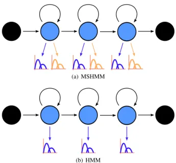
(a) MSHMM
(b) HMM
Figure 1:State diagram representation of a MSHMM compared to a regular HMM
2.3. Speech recognition modelling
The MSHMMs were trained using the HTK Toolkit [10] over the two training sessions. All models were trained on a topology of 13 states and 10 mixtures (each, for both audio and video), which was determined empirically to provide the best perfor-mance on the evaluation sessions.
For the training and testing of the MSHMM system, the closest video feature vector was chosen for each audio feature vector and appended to create a single 99-dimensional feature-fusion vector. No interpolated estimation of the video features between frames was performed.
For the purposes of these experiments, stream weightings for the MSHMMs were defined to beαfor the audio stream and1−αfor the video streams.
All models were tested for the task of small-vocabulary (digits only) continuous speech recognition on the XM2VTS dataset as outlined in Section 2.1. Speech recognition was per-formed on a simple word-loop with word-insertion penalties calculated for each system on the evaluation session. Speech recognition results were reported as a word-error-rate (WER) calculated by 1−H−I N ×100% (1) WhereH is the number of correctly estimated words,Iis the number of incorrectly inserted words, and N is the total number of actual words.
3. Stream weighting of MSHMMs
3.1. Multi-stream HMMsA MSHMM can be viewed as a regular single-stream HMM, but with two observation-emission Gaussian mixture models (GMMs) for each state–one for audio, and one for video– as shown in Figure 1. In the existing literature, MSHMMs have been trained in one of two manners: Two single-stream HMMs can be trained independently and combined, or the entire MSHMM can be jointly-trained using both modalities.
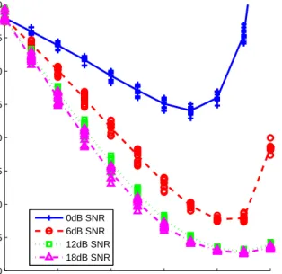
0 0.2 0.4 0.6 0.8 1 0 5 10 15 20 25 30 35 40 αtest
Word Error Rate
0dB SNR 6dB SNR 12dB SNR 18dB SNR
Figure 2:Speech recognition performance againstαtest. Each
point is a differentαtrain, and the lines show average WER for
eachαtest.
Because the combination method makes an incorrect assump-tion that the two HMMs were synchronous before combina-tion, better performance can be obtained with the joint-training method [11], and this is the method we chose for this paper.
As mentioned previously, the major benefit of MSHMMs over feature-fusion is the ability to weight either modality to represent its reliability. Therefore the choice of these weights is an important part in designing a MSHMM-based system. Much work has been done on the estimation of stream weights for decoding in various conditions [1], but due to the design of the MSHMM system the weights also have an effect on the training process, and the effect of these training weights has not yet been directly studied in the literature.
3.2. Speech recognition results
To investigate the effect of varying the training and testing weights independently, we conducted a large number of speech recognition experiments, as outlined in Section 2.3. 11 differ-ent training alphas, αtrain = 0.0,0.1, ...,1.0, and testing
al-phas,αtest = 0.0,0.1, ...1.0, were combined to arrive at 121
individual speech experiments. These experiments were then conducted over all 4 testing noise levels, resulting in a total of 484 tests. A plot of the WER obtained for each of these experi-ments againstαtestis shown in Figure 2.
From examining Figure 2 it can be seen that the variance in WER of the entire range ofαtrainis of little-to-no
signifi-cance to the final speech recognition performance. This can be seen more clearly in Figure 3, which shows the effect of varying
αtrainon the best performingαtestfor each noise level. Other
than the 0 dB SNR tests, which show a slight dip in error at
αtrain = 0.7, there appears to be no relationship between the
choice ofαtrainand the final speech recognition performance.
0 0.2 0.4 0.6 0.8 1 0 5 10 15 20 25 30 35 40 αtrain
Word Error Rate
0dB SNR (α test = 0.7) 6dB SNR (α test = 0.8) 12dB SNR (αtest = 0.9) 18dB SNR (αtest = 0.9)
Figure 3: Speech recognition performance againstαtrain for
the best-performingαtestin Figure 2.
3.3. Discussion
Training of HMMs is basically an iterative process of continu-ously re-estimating state boundaries (including state-transition likelihoods), and then re-estimating state models based on those boundaries. This cycle of (boundaries→models→ bound-aries) continues until there is no significant change in the pa-rameters of the estimated state models. The value ofαtrain
has no direct effect on the re-estimation of the state models, so the only effect of this parameter comes about when using the estimated state models to arrive at a new set of estimated state boundaries [10]. For example, ifαtrain = 0.0, then only the
video models determine the state boundaries during training. Similarlyαtrain = 1.0will only use the audio models, and
values between those two extremes will use a combination of both models for the task.
Because the speech transcription is known, training of a HMM is a much more constrained task than decoding unknown speech during testing. The 18dB SNR results presented in the previous section shows the decoding WER varies from around 3% for audio-only to a much higher 37% for video only, when the testing weight parameter,αtest, is set at the extremes of 1.0
and 0.0 respectively. That changing the training weight parame-ter,αtrain, has no similar effect on the final speech recognition
performance suggests that the video or audio models perform equally well in estimating the state boundaries during training, and there appears to be no real benefit to a fusion of the two during training.
4. MSHMM normalisation
Score normalisation is a technique used in multimodal biomet-ric systems that can be used to combine scores from multiple different classifiers [7] that may have very different score dis-tributions. By transforming the output of the classifiers into a common domain, the scores can be fused through a simple weighted sum of scores, where the weights can more accurately
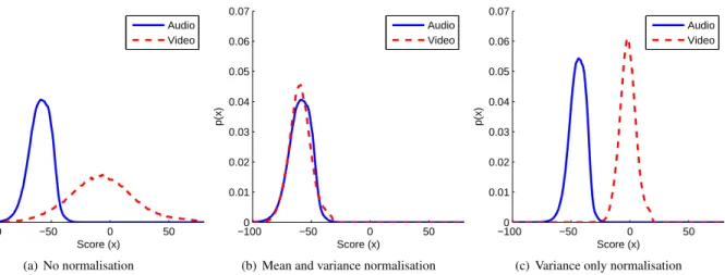
−1000 −50 0 50 0.01 0.02 0.03 0.04 0.05 0.06 0.07 Score (x) p(x) Audio Video (a) No normalisation −1000 −50 0 50 0.01 0.02 0.03 0.04 0.05 0.06 0.07 Score (x) p(x) Audio Video
(b) Mean and variance normalisation
−1000 −50 0 50 0.01 0.02 0.03 0.04 0.05 0.06 0.07 Score (x) p(x) Audio Video
(c) Variance only normalisation
Figure 4: Distribution of per-frame scores for individual audio and video state-models within the MSHMM under different types of normalisation.
represent the true dependence of the final score on the individ-ual classifiers. In this section, we will show how the concept of score normalisation can be used within a MSHMM to perform a similar function for audio-visual speech recognition.
4.1. Mean and variance normalisation
Before normalisation can occur within the MSHMM, the score distributions of the audio and video modalities first have to be determined. For our speech recognition system, we chose to use an adapted form of zero-normalisation [7]. Zero-normalisation transforms scores from different classifiers that are assumed to be normal into the standard normal distribution
N ∼ µ= 0, σ2= 1using the following function for each modalityi: Zi(si) = si−µˆi ˆ σi (2) wheresiis an output score from the classifier from
distri-butionSsuch thatS∼ µˆi,σˆi2
. The estimated normalisation parametersµˆiandσˆiare typically calculated on a left-out
por-tion of the data. Then during actual use or testing of the system, the final output score would be given by
sf =
X
i
wiZi(si) (3)
wherewiis the weight for modalityi, if desired.
For our speech recognition normalisation, we chose to adapt the video-score distribution to that of the audio-score, rather than perform zero normalisation on both distributions. This configuration was chosen because zero-normalisation would cause the state emission likelihoods to be much smaller than the state-transition likelihoods, causing the final speech recognition to mostly be a function of the latter. By using the audio-score distribution as a template, the final scores should be in a similar range to the state-transition likelihoods.
Before the video-normalisation could occur, the normalisa-tion parameters of both distribunormalisa-tions were determined by scor-ing the known transcriptions on the evaluation session with stream weight parameter,α, set such that only the modality of interest was being tested (i.e.α= 0andα= 1).
We also attempted to perform a full speech recognition task (rather than force alignment with a transcription) to calculate
Modality (i) Mean (µˆi) Standard Deviation (σˆi)
Audio -59.55 9.41
Video -7.07 27.88
Table 1:Normalisation parameters determined from the evalu-ation score distributions shown in Figure 4(a).
the distribution parameters, but no major difference was noted in the final parameters. This was most likely because the differ-ence between the two modality’s score distributions was much larger than any difference between the score distributions of dif-ferent state models within a particular modality.
The scores of the best path were then recorded on a frame-by-frame basis to determine the score-distribution of each modality, shown in Figure 4(a). The normalisation parameters, shown in Table 1 , were then estimated from the score distribu-tions for each modality.
To perform the video normalisation the output of the video-state models were first transformed to the standard normal dis-tribution, then to the audio distribution. The final score from the combined MSHMM state-model is given as
sf =αsa+ (1−α) sv−µˆv ˆ σv | {z } →N(0,1) × σˆa+ ˆµa | {z } →N(µˆa,ˆσ2 a) (4)
The effect of the transformation on the score-distribution can be seen in Figure 4(b). It can be seen that the audio score re-mains untouched, while the video scores have been transformed into the same domain as the audio.
Because this normalisation occurs within the Viterbi decod-ing process, we had to use our in-house HMM decoder to imple-ment this functionality, as it was not possible within the HTK Toolkit [10]. However, before discussing the results of our nor-malisation experiments, we will have a brief look at the possi-bility of normalising only the variances of the two distributions, as this can be performed solely with the weighting parameters already available in HTK.
4.2. Variance-only normalisation
Speech recognition is a comparative task, in that the model scores are only compared to each other and have no real
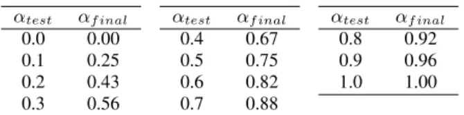
mean-αtest αf inal 0.0 0.00 0.1 0.25 0.2 0.43 0.3 0.56 αtest αf inal 0.4 0.67 0.5 0.75 0.6 0.82 0.7 0.88 αtest αf inal 0.8 0.92 0.9 0.96 1.0 1.00
Table 2: Final weighting parameter,αf inal, for intended test
parameter,αtestusingαnorm= 0.75.
ing external to that comparison. For this reason, a change in the mean log-likelihood scores on a stream-wide basis will have no effect on the ability to discriminate between individual word models, as they will all have their means affected similarly.
Therefore, if mean normalisation is not required, normal-isation can be more easily performed by considering the final modality weights (φa
f inal, φvf inal) to be a combination of the
intended test weights and calculated normalisation weights:
φaf inal = φ a test×φ a norm (5) φvf inal = φ v test×φ v norm (6)
Where the testing and normalisation weights can further be expressed in terms ofαtestandαnormrespectively:
φaf inal = αtest×αnorm (7)
φvf inal = (1−αtest) (1−αnorm) (8)
However, to ensure the state model emission likelihoods re-main in the same general dore-main as the state-transition like-lihoods, we need to ensure that the stream weights add to 1. Using (7) and (8) we can arrive at the final weight parameter,
αf inal = φaf inal φa f inal+φvf inal (9) αf inal = αtestαnorm
αtestαnorm+ (1−αtest) (1−αnorm)
(10)
To calculate the normalisation weighting parameterαnorm, we
use the following property of normal distributions,
kN ∼ kµ,(kσ)2 (11) and attempt to equalise the standard deviations of the two weighted score distributions:
αnormσˆa = (1−αnorm) ˆσv (12) αnorm = ˆ σv ˆ σa+ ˆσv (13)
Using the normalisation parameters from Table 1, we arrive at a normalisation weighting parameter of
αnorm=
27.88
27.88 + 9.41 = 0.75 (14)
Using our knowledge of the normalisation weighting pa-rameterαnormand the relationship shown in (9), we can map
any intendedαtestto the equivalentαf inalwhich will include
the effects of variance-normalisation, as shown in Table 2. The effect of this normalisation parameter on the unweighted score distributions is shown in Figure 4(c). It can be seen that the vari-ance of the two score distributions has been equalised, while the means are still very separate, although changed from the non-normalised score distributions.
4.3. Speech recognition results
To investigate the effect of normalisation on speech recognition performance, we conducted a series of tests at varying levels of
αtestfor both methods of score normalisation: mean and
vari-ance; and variance alone. These scores were conducted using the models trained in Section 3 with the training weight param-eter ofαtrain= 0.7. As discussed in Section 3.3, the choice of
the training weight parameter was fairly arbitrary, but 0.7 was chosen as it had the lowest average WER over all noise levels by a minor margin.
The results of these experiments are shown for the audio SNRs of 0, 6 and 12 dB in Figure 5. 18 dB was not included due to space constraints, but was not significantly different from the 12 dB graph shown. The non-normalised performance of
αtrain= 0.7calculated in Section 3.2 has also been included
for comparison.
4.4. Discussion
From examining Figure 5, it can be seen that both normalisation methods are very similar about the best-performing section of the curve. However, it would appear that, at least in this case, normalising the video scores into the range of the audio scores improves the video-only performance (5% WER decrease at
αtest = 0.0). It is not entirely clear at this stage what causes
this improvement, but it is likely a side-effect of the interaction of the transformed video scores and the state-transition likeli-hoods, and it is not clear if it would always be in favour of the mean-and-variance normalisation.
From the results in Figure 5 and the αtest → αf inal
variance-normalisation mappings shown in Table 2, we can see that normalisation is essentially moving the center of theαtest
range closer to the best-performing non-normalisedαtest, and
also producing a flatter WER curve around this point. These results show that the main effect of the best-performing weight-ing parameter ofαtest≈0.8from our earlier weighting
exper-iments primarily serves to normalise the two modalities rather than indicate their impact on the final MSHMM performance. The best-performingαtestin either of the normalised systems
is much closer to 0.5, indicating that both modalities are con-tributing almost equally to the final performance.
5. Conclusion and future research
In this paper we have shown that the choice of stream weights used during the training process of MSHMMs is far less im-portant than the choice of stream weights used during decod-ing. For the particular case of training being performed in a clean environment, we have shown that there is no real differ-ence between any particular combination of stream weights on the final speech recognition performance. While there was a considerable difference in the audio or video only performance in decoding, both appear to work equally well in determining the state alignments during the joint training process, and no increase was noted for any combination of the two.In our stream weighting experiments, we showed that the best speech recognition performance was obtained when the models where combined within the MSHMM at around 80% audio and 20% video. However, by performing normalisation of the audio and video score distributions within the MSHMM states before combining the two models, we have shown that the true dependence of the final system on each modality is much closer to 50% each. The normalisation performed was a novel adaption of zero-normalisation to MSHMMs, and we
0 0.2 0.4 0.6 0.8 1 0 5 10 15 20 25 30 35 40 αtest
Word Error Rate
None Variance Only Mean and Variance
(a) 0 dB SNR 0 0.2 0.4 0.6 0.8 1 0 5 10 15 20 25 30 35 40 αtest
Word Error Rate
None Variance Only Mean and Variance
(b) 6 dB SNR 0 0.2 0.4 0.6 0.8 1 0 5 10 15 20 25 30 35 40 αtest
Word Error Rate
None Variance Only Mean and Variance
(c) 12 dB SNR
Figure 5:Speech recognition performance under normalisation. 18 dB SNR was not included as it was very similar to 12 dB SNR.
also presented an alternative variance-only normalisation that can be implemented solely through adjusting the stream weights to achieve much the same results.
Some of our future research in this area will investigate whether MSHMM training can be performed by training video state models directly from state alignments generated by an audio HMM. As our training weight experiments here have shown, the state-alignment should be as good as any a MSHMM would arrive at, and by training the video state models directly there would be no chance of re-estimation errors being intro-duced into these models. This work will be based on our exist-ing work with Fused HMMs [12].
In addition, although we have not presented normalisation as a method of stream weight estimation in this paper, it would appear that normalisation could play a valuable part in this area of research. Instead of viewing the normalisation as an internal part of the MSHMM, one could use the variance-only normal-isation method to produce a good estimate of the optimal non-normalisedαtest, which could be used as a starting point for
more sophisticated stream-weight estimation.
6. Acknowledgments
The research on which this paper is based acknowledges the use of the Extended Multimodal Face Database and associated documentation. Further details of this software can be found in [8] or athttp://www.ee.surrey.ac.uk/Research/ VSSP/xm2vtsdb/.
7. References
[1] G. Potamianos, C. Neti, G. Gravier, A. Garg, and A. Se-nior, “Recent advances in the automatic recognition of au-diovisual speech,”Proceedings of the IEEE, vol. 91, no. 9, pp. 1306–1326, 2003.
[2] Y. Gong, “Speech recognition in noisy environments: A survey,”Speech Communication, vol. 16, no. 3, pp. 261– 291, 1995.
[3] H. McGurk and J. MacDonald, “Hearing lips and seeing voices,” Nature, vol. 264, no. 5588, pp. 746–748, Dec. 1976. [Online]. Available: http://dx.doi.org/10.1038/ 264746a0
[4] S. M. Thomas and T. R. Jordan, “Contributions of oral and extraoral facial movement to visual and audiovisual speech perception,”Journal of Experimental Psychology: Human Perception and Performance, vol. 30, no. 5, pp. 873–888, 2004.
[5] S. Bengio, “Multimodal speech processing using asyn-chronous hidden markov models,” Information Fusion, vol. 5, no. 2, pp. 81–9, June 2004.
[6] A. Nefian, L. Liang, X. Pi, L. Xiaoxiang, C. Mao, and K. Murphy, “A coupled hmm for audio-visual speech recognition,” inAcoustics, Speech, and Signal Process-ing, 2002. Proceedings. (ICASSP ’02). IEEE International Conference on, vol. 2, 2002, pp. 2013–2016.
[7] A. Jain, K. Nandakumar, and A. Ross, “Score normaliza-tion in multimodal biometric systems,”Pattern recogni-tion, vol. 38, no. 12, pp. 2270–2285, 2005.
[8] K. Messer, J. Matas, J. Kittler, J. Luettin, and G. Maitre, “XM2VTSDB: The extended M2VTS database,” in Au-dio and Video-based Biometric Person Authentication (AVBPA ’99), Second International Conference on, Wash-ington D.C., 1999, pp. 72–77.
[9] J. Luettin and G. Maitre, “Evaluation protocol for the ex-tended M2VTS database (XM2VTSDB),” IDIAP, Tech. Rep., 1998.
[10] S. Young, G. Evermann, D. Kershaw, G. Moore, J. Odell, D. Ollason, D. Povey, V. Valtchev, and P. Woodland,The HTK Book, 3rd ed. Cambridge, UK: Cambridge Univer-sity Engineering Department., 2002.
[11] C. Neti, G. Potamianos, J. Luettin, I. Matthews, H. Glotin, D. Vergyri, J. Sison, A. Mashari, and J. Zhou, “Audio-visual speech recognition,” Johns Hopkins University, CLSP, Tech. Rep. WS00AVSR, 2000. [Online]. Available: citeseer.ist.psu.edu/neti00audiovisual.html
[12] D. Dean, S. Sridharan, and T. Wark, “Audio-visual speaker verification using continuous fused HMMs,” in