Costs of Deep Geothermal Energy in the Netherlands

(1)

MSc Sustainable Development

Thesis

Costs of Deep Geothermal Energy in the Netherlands

Derk Straathof

June 30

th

, 2012

ECN-O--12-043

(2)

Contact Information

Author Derk Straathof

Sustainable Development; Track Energy & Resources Utrecht University

Supervisor UU Dr. Robert Harmsen

Assistant Professor Energy & Resources

Department of Innovation and Environmental Sciences Faculty of Geosciences

Utrecht University

Email: r.harmsen@geo.uu.nl

Telephone: +31 (0) 30 2534419 Second Reader Drs. Sander van Egmond

Project Manager, Utrecht Centre for Energy Research Utrecht University

Email: s.vanegmond@uu.nl

Telephone: +31 (0)30 2537529 Supervisor ECN Paul Lako, MSc

Senior Research Fellow, Policy Studies Energy research Centre of the Netherlands

Email: lako@ecn.nl

Telephone: +31 (0)88 5154418 Supervisor TNO Prof. Jan-Diederik van Wees

Senior Researcher, Sustainable Geo-energy TNO Bouw en Ondergrond

Email: jan_diederik.vanwees@tno.nl Telephone: +31 (0)88 866 49 31

(3)

Abstract

The costs of deep geothermal energy in the Netherlands are analysed. A database is constructed using data from the existing projects in the Netherlands and nearby countries, producing an equation for costs of drilling. A model is developed in Java, building on prior models developed by TNO, using the methodology for calculating SDE+ subsidies by ECN. This model primarily calculates the Unit Technical Costs of deep geothermal projects. This allows for rapid assessment of the economic attractiveness of locations and quick comparison to the SDE+ base rates for possible subsidy applications.

Foreword

Much of this research would not have been possible without the internships I followed at ECN and TNO. The following paragraphs give a short description of how my internships came about and are also for readers who are not acquainted with these organisations.

ECN

ECN is the Energy Research centre of the Netherlands, located in Petten, with ancillary locations in Amsterdam, Brussels, and Beijing. It was developed around the small experimental nuclear reactor at Petten to research new energy technologies. As such, it performs cutting edge research on solar, wind, biomass and energy efficiency technologies. In addition to these more laboratory-based fields of research, there is a Policy Studies unit which does primarily research from a policy/economic point of view and from the point of view of social sciences, usually through building models and scenarios and writing papers and advices. Into this unit I was invited to research geothermal energy as an intern. As geothermal energy is not at the heart of research at ECN, knowledge of this energy technology is limited and ECN does not have much on offer today for development of geothermal energy. My supervisor was Paul Lako, a senior researcher in the Policy Studies department, who had worked on advice for the SDE+ subsidy in 2011.

TNO

TNO is the Netherlands Organisation for Applied Scientific Research. It performs a frontline research role in many areas, primarily for the Dutch government, which provides significant funding. One of TNO’s responsibilities, through its DINO and NLOG sectors, is collating the known information of seismic and core data resulting from oil and gas research. With the expertise that came with this responsibility, it was natural for TNO to also start performing research into geothermal energy, as there are many similarities between the two. Jan-Diederik van Wees is a senior researcher in the Sustainable Geo-Energy unit, and also works at the University of Utrecht in the Geosciences department. After interviewing him in the course of my internship at ECN, it became clear that collaboration between ECN and TNO would be very useful, with my internship as its fulcrum. TNO possesses great knowledge of the subsurface, and ECN Policy Studies has important expertise from the economic and policy side. It was thus decided that I would also be a guest intern at TNO alongside my internship at ECN.

(4)

Dedication

This one is for my dad, Dirk Jan Straathof. I wish you were here to read it.

Acknowledgements

This thesis was written during an immensely difficult time for me, and I’m incredibly grateful for all the help and support I received during this time. In particular, I want to thank the many colleagues at ECN and TNO who made working there so interesting and so much fun. Also, I strongly appreciate all the people who graciously allowed me to interview them, who answered my queries and brought me in contact with the required expertise. However, certain people deserve special recognition:

Robert, for being my supervisor and getting this project started, and helping me out in times of trouble.

Paul, also for being my supervisor, and for the many discussions, debates and of course the Lange Afstand Loop!

Jan-Diederik, who was also my supervisor, for accepting me at TNO and allowing me to build on the tremendous work they have already accomplished.

Maarten, for helping me significantly with Java, and with my badge at TNO! Marloes, my fellow intern, with whom I learned to write in Java together. And of course I want to thank my family and friends, for everything. Last but not least, I can’t forget Yvonne, who is simply amazing!

(5)

1 Introduction

Geothermal energy refers to energy contained within our planet Earth. The etymology derives from ancient Greek, where “geo” refers to Earth and “therme” to heat. In general, the Earth can be regarded as a sphere, with the Earth’s interior warmer than its surface. The surface is a suitable temperature for human and all other life as we know it, but relatively speaking, it is the coldest part of the Earth. The far hotter interior has heat which originates from the residual heat of formation of the Earth, as well as the decay of radioactive isotopes. It is thus theoretically possible to utilize this temperature differential to produce useful energy.

The Earth can be considered nearly spheroid in shape, with a radius of about 6370 km. Along its radius, there are three identified zones, defining concentric spheres: the core, the mantle and the crust. The innermost is the core, with a radius of 3470 km. It is predicted to have a temperature of at least 4000°C, and a pressure of at least 360,000 MPa. However, this has not been proven empirically, as human technology is thus far incapable of reaching such depths. (Barbier, 2002)

In fact, human technology cannot even reach the second layer, the mantle, which is about 2900 km thick and consists of very hot rock. The outermost layer is the crust, on which we reside, which is also the thinnest: it varies from about 7 to 65 km in thickness. This layer is also the coldest, as the heat that conducts from the interior is passed from here to the atmosphere and then space. (Barbier, 2002) Fortunately for humans, the atmosphere’s natural greenhouse effect keeps the surface warm enough to be survivable. Only the top ten meters or so of soil are susceptible to changes in

atmospheric temperatures, and are for the Netherlands characterised by an average temperature of 10°C. Below that, the Earth’s crust warms up as one gets deeper, on average by about 30°C/km, although this can vary from 10-100°C/km depending on location. (Tester et al, 2006, Rogge, 2003)

1.1 Technologies

There are several technologies, which fall under geothermal energy in common parlance. It thus becomes necessary to define the types examined in this thesis. The following technologies can all be categorized as geothermal energy, in that they extract energy from the ground:

1. geothermal heat pumps, which extract heat from the shallow underground by taking advantage of a heat pump

2. heat and cold storage, which stores heat during the summer and cold during the winter in shallow underground reservoirs

3. volcanic geothermal, which extracts heat from natural shallow hotspots and is only feasible near volcanoes and the edges of tectonic plates

4. deep aquifer, which involves a borehole drilling deep into the earth to extract warm water from an aquifer (also known as a hydrothermal system)

5. enhanced geothermal systems (EGS), the successor of hot dry rock, which usually drills even deeper but also has to fracture rock to allow water flow.

These technologies fall roughly into two families: the former two are shallow, relatively small scale, and very low temperature technologies, and the latter three are deeper, larger scale higher

(8)

systems which are not applicable for the Netherlands due to its lack of tectonic activity, will not be addressed in this report. Instead, the focus will be on the deep technologies: aquifer (hydrothermal system) and EGS.

1.2 Deep geothermal

The primary system under investigation is deep aquifer geothermal (hydrothermal system). An aquifer is an underground layer of porous rock, such as sandstone, which bears water in the pores. With the temperature rising by around 31°C /km depth, an aquifer at two kilometres deep will typically have a temperature of around 70°C. This water is at a useful temperature for many

residential and horticultural applications. Should such an aquifer be available beneath the customer of interest, it can be interesting to drill for geothermal energy. Apart from a sufficiently high

temperature, the aquifer will also need to have a suitable transmissivity, which is defined as

The thickness of the aquifer is the height of the aquifer, as long as this is contiguous, not broken by sealing faults or other layers of less porous rock. The permeability is a measure of how easily water flows through the pores of the rock structure, and is roughly related to porosity. If the transmissivity is high enough, a sufficient flow rate can be established for the topside purposes. Of the two critical characteristics required for geothermal energy, transmissivity is often harder to guarantee

beforehand than temperature for a prospective exploiter.

If the aquifer is thought to be suitable, it can be accessed by a well. The well is drilled from the surface and extracts water through a pump and a pressure differential. To maintain aquifer pressure, a second well is needed to reinject water. The reinjected water is at a lower temperature for

thermodynamic reasons. The temperature differential between the extracted and injected water is used to extract useful energy. A pair of wells, consisting of an injection and a production well, is known as a doublet. If the water is between 60°C and approximately 100°C, this can only be used for heating, considering the economics of geothermal power generation.1_{Thus a heat exchanger is} installed and the heat of the subsurface water transferred to fresh water above ground. This fresh water is used for whatever purpose required, and the now cooler geothermal water is injected back into the aquifer completing the closed loop. At no point is the geothermal water exposed to the open atmosphere, and thus no gases escape to the atmosphere and there should be no contamination of the aquifer during operation.

1.3 Enhanced Geothermal Systems and Electricity Production

To generate electricity, temperatures of at least 130°C are preferred. Thermodynamically speaking, the temperature should be as high as possible, provided that the technology to access geothermal prospects with such high temperatures is commercially available. In other words, to reach such temperatures, one needs to drill deeper, as per the previously defined temperature gradient. However, pressures at these depths are also greater, as there is more overbearing rock. This extra pressure usually reduces the porosity of rock layers, which in turn reduces the transmissivity.

Therefore, there are few aquifers with temperatures in the range usable for electricity generation. In

1

One small power plant in Chena, Alaska uses 73°C water to produce electricity, but this is an exceptional case. (Holdmann, 2007)

(9)

this case, a suitable reservoir situation has to be stimulated. This is what Enhanced Geothermal System (EGS) means. A process known as fracking is used to create multiple fractures in the hot dry rock. These fractures can be carefully controlled and directed, and create the necessary porosity and transmissivity for a usable geothermal source. With the rock between the injector and producer well suitably fractured, water can flow between the two. This water returns to the surface at a high temperature and can be used for the desired purpose.

Whether EGS is used or not, if the temperature of the water is high enough, it can be used to produce electricity via a turbine. Sometimes, both electricity and heat are produced in what is called a Combined Heat and Power (CHP) facility. Several types of electricity producing facilities are possible for geothermal power, but all involve a generator producing electricity being turned by a gas heated geothermally. At low temperatures (<130°C) it is best to use a binary system like either a Kalina cycle or an Organic Rankine Cycle (ORC). These cycles are called binary because the hot geothermal water transfers the heat in a heat exchanger to a secondary liquid (sometimes called the working fluid). The working fluid evaporates with this heat, and this gas goes into the turbine. The turbine drives the generator, and electricity is produced. In a Kalina Cycle, the working fluid is an ammonia and water mix, and in an ORC, the working fluid is one of many organic liquids. Both can be calibrated

specifically for the particular geothermal plant so that the optimum efficiency is reached.

At higher temperatures, it is more common to use flash or dry steam cycles (sometimes in tandem with an ORC) to produce electricity, because they are more efficient. Both of these cycles do not use a secondary liquid, but the geothermal liquid itself is used. This can be more damaging to the turbine and can result in the escape of undesired gases.

After the heat is extracted from the geothermal water, it is pumped back into the aquifer through the injection well. The pumps require electricity which can either come from the geothermal plant (if it produces electricity), when it will be called parasitic demand, or it needs to come from an external source.

For further information on electricity generation for geothermal power, Rogge (2006) and Koehler (2006) are recommended.

2 Problem definition

The ever-increasing consumption of fossil fuels as an energy source is not sustainable for two main reasons. Firstly, fossil fuels are non-renewable, and while plentiful, will become increasingly more expensive to discover and produce. Secondly, there are dire environmental consequences resulting from the combustion of fossil fuels. The most fearsome is global climate change, which is the worldwide disruption of climatic patterns due to excess heat trapped in the Earth’s atmosphere by the so-called greenhouse gases, chief among them carbon dioxide. However, other consequences include rising acidity of bodies of water and soils, smog, release of particulates harmful to human health and oil spills such as in the Gulf of Mexico recently. While some technological and policy solutions have been developed for some of these issues, such as catalytic converters and NOx and SO2 reduction (desulphurization) in coal-fired power plants, it is clear that a structural energy

(10)

This has led to the rise of renewable energy sources, primarily wind, solar and biomass. A reliable energy source which happens to be out of the spotlight is geothermal energy. This is despite some obvious advantages geothermal has over other energy sources. Compared to biomass and fossil fuels, geothermal is advantageous in that it has no fuel costs, and fuel does not need to be

transported. Also, there are very few emissions of greenhouse (or other harmful) gases associated with geothermal energy. This is especially true for the closed-loop doublets used in the Netherlands. Conversely, fossil fuels and biomass both directly emit greenhouse gases such as carbon dioxide (albeit without net CO2 emission if biomass is grown sustainably), as well as other emissions such as nitrous oxides and sulphur dioxide, which need to be sequestered with filters. Compared to solar and wind power, two high-profile renewable energy sources, geothermal is advantageous because it provides constant base-load energy, it occupies very little surface space, and it has a long lifetime. The first is a major advantage: wind and solar energy do not operate constantly, perhaps 2500 (wind) to at most 4000 (solar) hours in a year, and then not always at predictable or useful times.

Geothermal can reliably produce energy for at least 7500 predictable hours if there is demand. The second is a smaller advantage, but still worth mentioning. Wind energy requires large, highly visible turbines. Solar energy requires a great deal of south-facing, shadow-free surface area. In comparison, geothermal requires a small building once it is installed, although the construction phase does require an area of about a football pitch. There are two main disadvantages keeping the widespread development of geothermal energy back from fulfilling its potential: high and uncertain investment costs, and technological and geological uncertainty regarding production levels of energy.

It is therefore the intention of this report to investigate the costs of geothermal plants, and create a flexible model that can provide an assessment of these costs at various locations and incorporate the inherent uncertainty to produce a useful financial estimate.

2.1 Research Question

With that goal in mind, this research project investigates the following research question:

What are the costs of deep geothermal heat and power in the Netherlands now and over the next 30 years?

The costs should be determined in absolute costs per project, and then evaluated for several factors, including cost/depth (in €/m) and cost of energy (in €/kWh or €/GJ). Initially, a simple empirical trend of past and current costs can be developed, but the final result is an integral analysis of all costs involved in the project, with uncertainty ranges and variations depending on relevant factors. Costs should include the initial investment costs (including cost of exploration, drilling, and production of the wells), and fixed and variable operation and maintenance costs.

2.2 Research sub-questions

What factors decide the costs of a project, and what influence do they have?

For the initial investment, in particular the costs of depth and breadth of wells are analysed, in addition to the costs of capital and insurance. Furthermore, an assessment of the operational and maintenance costs is needed. Moreover, the influence of the market should be evaluated,

(11)

particularly the influence of the prices of oil and gas (which may impact on the drilling costs), and steel (which will influence material costs).

The investment costs also include the equipment needed to provide the desired product (heat, electricity or both) to the location, which could range from a simple heat exchanger for horticultural purposes, to an entire district heating network, to an Organic Rankine Cycle. Each of these scenarios should be examined.

What influence do government policies have on the costs?

Current government policies such as the MEI and UKR are incidental investment subsidies. The potential SDE+ subsidy is now for both heat and electricity, what kind of shift in investment can this cause? Can such subsidies encourage wavering project planners to make the investment jump? Or are the incidental subsidies and the (adjudged to be) expensive guarantee fund not sufficient? How do the costs of drilling compare to the costs abroad?

Are the many realised projects in Germany, France, and the U.S.A. comparable in nature to potential Dutch projects? What differences are there (in geological, economic and policy terms) and how do these affect the costs?

How will delays affect the costs?

A common issue with projects appears to be delays before, during and after drilling. How much do these delays cost the project owners?

2.3 System Boundaries

The scope of this project is deep geothermal energy in the Netherlands over the next 30 years. “Deep” means, by law, deeper than 500 m from the surface, but to be commercially attractive it generally refers to at least 1500 m deep. Geothermal refers to the residual heat of formation and the heat from radioactive decay in the Earth’s core. Although current technologies are only capable of reaching several kilometres into the crust, it is still far warmer than the surface. The energy derived from this is extracted from the subsurface in the form of warm water (either liquid or gaseous depending on the conditions), and either heat or electricity, or both, can be derived from this carrier. Current Dutch applications are mainly heat for horticultural and residential purposes (district

heating), but others are possible.

The project looks specifically at current and future geothermal heat and power in the Netherlands. However, comparisons are drawn to geothermal power in other countries, especially (nearly) neighbouring countries like France and Germany. This is because more or a similar number of projects have been realized in these countries, providing more experience and data. These can be compared and contrasted with the Dutch situation.

Of the several different types of geothermal power, this project will focus mainly on aquifer systems, as these are the ones currently in use in the Netherlands at the time and those being developed. Enhanced Geothermal Systems will also be looked at, because while these are not in use at the

(12)

moment, they do appear to be the future system of choice next to more shallow geothermal energy systems used for heating.

The technical boundaries of a system include the underground source, the injection and production wells, and any surface installations for converting and transporting the energy to the existing demand. This includes heat exchangers and turbines. However, it is mainly the economic side of a project that is investigated.

2.4 Previous work

When researching the literature of geothermal energy, it quickly becomes clear that the seminal work in this section is that of Tester et al, an MIT study in 2006 performing a large-scale economic analysis of deep geothermal energy in the United States of America. The 12 co-authors are all experts in the field and have written often on the topic. Tester et al provides a strong, detailed analysis of geothermal energy, including the costs and how these have developed over time. One of the key results is that there has been a tremendous increase in costs since the early 2000’s.

The main reasons why this work is needed when Tester et al has already been published is because geothermal energy in the Netherlands is not developed in the same manner as the Unites States. The USA primarily derives geothermal energy from aquifers in volcanic conditions. These tend to be shallower and hotter than Dutch reservoirs. Additionally, they tend to be more remote and thus useful for electricity production but not heat production, whereas Dutch geothermal energy thus far is all in the form of heat. This resulted in a wholly different approach to geothermal energy in the USA compared to the Netherlands. It is not uncommon in the USA to perform “wildcat” drillings, which have only a 25% success rate. In contrast, in the Netherlands drilling will not start until all available information has been collected and the greatest possible knowledge of the situation is available.

In the Netherlands, significant research has been performed by TNO. The model ThermoGIS is a model which provides a map of subsurface water reservoirs (also known as aquifers) in the Netherlands. This information is derived from the known seismic and well data that has been provided to TNO. As such, it can make estimates of all the important data for aquifers at a given location, such as temperature, thickness, depth and permeability. This information is used to calculate a likely heat in place and potential recoverable heat for a well at a particular location. An attached economic module called DoubletCalc determines the cost and other economic aspects of such a project. For in-depth description of ThermoGIS and DoubletCalc, Kramers, et al (2012) and van Wees, et al (2012) are recommended.

ECN Policy Studies is responsible for advising the Ministry of Economic Affairs on subsidy issues (SDE+), in collaboration with KEMA (a private consultancy owned by DNV). The SDE+ scheme (a subsidy named Besluit stimulering duurzame energieproductie +) has been expanded in 2012 to include projects delivering heat as well as projects delivering electricity and green gas. As a result, significant new research was needed on the costs of renewable technologies delivering heat, in particular geothermal heat.

(13)

3 Methodology

This chapter presents the two products that will lead to answering the research questions. First, a database is compiled, and then a model is developed. The approaches to these two products are briefly described.

3.1 Database

To determine the cost of geothermal energy in the Netherlands, it was decided to first develop a database of recently completed geothermal projects. This was done for several reasons. First, it gave a good indication of the state of the technology and the economic dimension. Secondly, it provided a useful cache of case studies for both the author and ECN. Thirdly, it allowed for a test of the drilling cost results of Tester et al (2006) and van Wees et al (2009) as they apply to the current Dutch situation. Fourthly, it allows some measure of comparison between the Dutch facilities already developed, and similar facilities in nearby countries.

This database contains publically available information on these projects, with a key emphasis on the technical and economic aspects, especially depth, production capacity and cost. Microsoft Excel proved to be a useful tool for making such a database.

The database builds on data gathered in Lako et al (2011), and is supplemented by an in-depth literature and news article search. Projects are identified first through national geothermal

organisations, such as Stichting Platform Geothermie for the Netherlands, and then researched using a search engine for news articles and websites which contain relevant details. Care needs to be taken to identify discrepancies between articles. Usually, in such cases, the quality of the source is

assessed, and the point in time it was authored. A later report will probably have a more complete picture of the investment costs.

Selected projects are primarily recent (since 2002), and in Europe in non-volcanic conditions. The choice of timeframe is because literature (Tester et al, 2006) and discussions with experts shows that since about this time, the cost of drilling has been dramatically higher. This rise is attributed to a rise in the price of oil, a diminishment in the number of drilling rigs and the advent of shale gas drilling. Thus, comparison with older geothermal projects is not helpful in predicting costs of future and current projects. The choice of locations limits projects to primarily those in the Netherlands and Germany, with a few projects in France, Denmark and Hungary. Not included are projects in Iceland or Italy, where volcanic subsurface conditions mean wells are significantly less deep, and other equipment is needed to deal with the higher temperatures. Also not included are projects in Turkey or Eastern Europe, where costs of labour are lower and thus not representative of projects in the Netherlands. Projects in Germany and neighbouring countries are legitimately included, as many drilling companies operate in both countries. Drilling rigs can be easily transported in containers by trucks.

Data on the projects comes from publically available sources, including national geothermal databases if accessible, media reports, company websites and publications. While there may be some scepticism regarding the accuracy of such data, there is little reason for this. Many projects are by small companies that only intend to develop one source, and thus there is no reason for them to

(14)

requirement of government subsidies and permits. Thus there is little uncertainty in technical and geological data. One area that is generally vaguer is the costs, as there are competitive reasons to keep this general, especially for drilling companies. Furthermore, the costs that are quoted tend to be rounded off to the nearest million. However, as most projects cost at least 10 million euro, this means the uncertainty for cost figures is less than ten percent. The reliability of these statements can be checked if there are multiple sources available, or perhaps if there are preliminary studies.

Overall, the end results are expected to be accurate enough for this research.

Once the database has been built and filled with projects, trends and patterns can be evaluated. This includes, but is not limited to, average costs per meter, average cost per kWh, costs developing over time, and that per country and depth category. These trends and costs can be inserted into the model developed in the second stage.

3.2 Modelling

As the results of the database will show, there is not yet a significant amount of data available to empirically answer many of the sub-questions to the research question. There is a great deal of uncertainty involved and every geothermal site is different. An effective way to handle that is to develop a model. A successful model will be user-friendly, allowing the user to set variables. Such a model is flexible enough to adapt to different geotechnical and economic situations and should have the capacity to answer the various research sub-questions.

The language of the model was a difficult decision. Given the author’s past experience, a model in Excel seemed the most probable way forward. However, a meeting with the Sustainable Geo-energy group at TNO, a group which had already accomplished significant model development in Java, led to the decision to write this model in Java, expanding on the expertise and knowledge at that institute. Java is a programming language, and is written and manipulated using a programme called Eclipse, which provides a sort of digital workbench. The result is a model called DoubletCalc, which performs geotechnical and economic calculations. TNO already had an early version of DoubletCalc, see van Wees et al (2010), and have also produced a new version recently (van Wees et al, 2012).

4 Results

This chapter provides an overview of the results that have been obtained in the research project. First, the results from the database are presented. Next the model is described in several stages. First, the way it was put together, by presenting the changeable variables and the calculations that operate on them. Then the user interface is shown, along with a typical, hypothetical project. Finally, the model is tested using available data for two potential projects.

4.1 Database results

The section describes the main results from the database. The database includes 62 deep geothermal installations that have recently been built in the Netherlands and other European countries which

(15)

have reasonably similar subsurface conditions as the Netherlands. Of these, 34 have publically available drilling cost totals which are considered reliable. These 34 geothermal projects are thus used in the analysis to follow.

Most (27 out of 34) of the facilities are used exclusively for heating. In general, these projects are cheaper as the wells are less deep and the installations do not require a turbine. However, plants where the heat is used for district heating can carry significant network construction costs with them. Of the 27 projects only producing heat, 20 are for district heating, six for greenhouses and 1 for heating an airport. Interestingly, all the greenhouse projects are in the Netherlands.

Six of the 34 projects are for CHP, with the majority using that heat for district heating or in a cascade system for nearby buildings. Just one project only produces electricity, and that is the experimental Soultz project (France), which tested EGS.

It should be clear that the database is not exhaustive. This is indicated by the mere fact that nearly half the projects, (28 out of 62) are not used in the analysis because there is not enough publically available information on them. Furthermore, some of the data, especially costs, has a significant uncertainty margin due to the nature of the reporting. However, it does provide an interesting indication of the state-of-the-art costs, and the current trends.

4.1.1 Country divisions

The figure below shows in which European countries the 34 geothermal projects in the database have been realized:

Figure 4.1 Division of projects in database by country.

The sample is thus clearly mostly based on German projects, though the Netherlands is also well represented in the database.

4.1.2 Cost per meter

One of the key results of the database is the relationship between drilling costs and depth of the well as shown in the figure below.

0 2 4 6 8 10 12 14 16 18 20

Austria Denmark France Germany Hungary Netherlands

N u m b e r o f p ro jec ts

(16)

Figure 4.2a and b Cost of drilling over depth of well, and b) cost of drilling divided by country.

Figure 4.2a shows thirty-four data points. The most accurate equation for a trendline is displayed. The figure shows that there is a general relationship between cost and depth: deeper wells tend to be more expensive in terms of drilling costs. However, the R^2 value of 59% indicates that while depth is linked with costs, the relation is not strong. The smallness of the error bars indicates that the weakness of the relationship between depth and drilling costs is not due to the uncertainty of the data points. y = 1E-07x2_{+ 0,0018x + 0,3859} R² = 0,596 0 2 4 6 8 10 12 14 16 0 1000 2000 3000 4000 5000 6000 Co st o f d ri lli n g [M e u ro ] Depth of well [m]

Cost of drilling

0 2 4 6 8 10 12 14 0 1000 2000 3000 4000 5000 6000 Co st o f D ri lli n g [M e u ro ] Depth [m]

Cost of Drilling Trendlines divided by Location

Germany R² = 0,5363 Other European R² = 0,7884 Netherlands with outlyer R² = 0,4258

(17)

Figure 4.2b shows that same data, divided by country. To protect possible confidentiality of projects, only the resulting trendlines are shown. Again, the R^2 values are small, indicating a poor fit between trendlines and data points. The Dutch curve is of particular interest.2 It has been shortened because there are no data points above 3000 m depth, but it appears to shrink with depth. This can be attributed to insufficient data, as there are only 7 data points, and these are of relatively shallow depths. Given the proximity of the lines, it could be expected that with more projects, the curve will resemble those of other European projects. The German and ‘other European’ trendlines are surprisingly similar.

4.1.3 Cost per capacity

The figure below shows the relationship between output capacity and the cost of drilling.

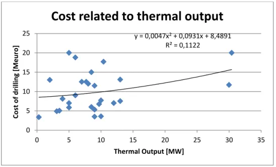
Figure 4.3 Cost of drilling over thermal output.

The data points in the figure show that the relationship between drilling costs and thermal output is not strong at all since the R^2 value is only 11%. The relationship between thermal output and drilling costs is not significant, especially compared to the relationship between depth and cost of drilling and depth. Nonetheless, this relationship is still commonly mentioned in reports. From this result, it appears clear that if a cost equation is needed to describe a geothermal facility, this is better done through a cost per depth formula than cost per output.

4.2 Model Development, Calculations and Output

The model is effectively the major result of this project. Thus the construction, testing and results from the model are all listed here, in one consecutive section.

My alternative version of DoubletCalc builds upon the model developed by TNO (Van Wees, et al, 2010, 2012) and is written entirely in the programming language Java. This alternative model comes

2

One curiosity is that six of the points form a line with an R^2 value of 96%. This is a surprisingly close correlation between depth and costs of drilling. However, the projects are mostly of similar depth and this is

y = 0,0047x2_{+ 0,0931x + 8,4891} R² = 0,1122 0 5 10 15 20 25 0 5 10 15 20 25 30 35 Co st o f d ri lli n g [M e u ro ] Thermal Output [MW]

(18)

in two versions: Heat and CHP (combined heat and power). The Heat version is more narrow and streamlined towards use by horticulturalists, and has the most recent TNO update on the geotechnical side (van Wees et al, 2012). The Heat version is also intended to be linked to the

ThermoGIS model which is currently being revamped by TNO. The CHP version is designed for a more academic purpose, as it is very unlikely that the geothermal CHP market will develop strongly in the near future. However, this means the CHP model is also used to try out a few experiments such as overland pipelines and delay effects.

4.2.1 The Heat Model Variables

The user interface of DoubletCalc allows the user to manipulate nearly all variables, and thus many results can be produced. The geotechnical variables were developed by TNO and are shown in Appendix B. Further information on them can be found in van Wees et al (2012). The economic variables that are changeable are shown in the tables below. Key among these are geotechnical variables such as depth, porosity and temperature, and lifetime, interest and debt-equity ratio as economic variables.

Changeable Economic variables

Economic lifetime the expected lifetime of the plant, mainly dependent on equipment and the aquifer

Pump replacement frequency

one major operational cost is the frequent replacement of pumps, especially the ESP in the production well. This variable caters for that need.

Heat exchanger season factor

the season factor is the fraction of the year that the plant is operational Load Hours derived from the season factor, represents the number of hours per

year the plant is on

Electricity price to buy the range of the expected costs of electricity, which is needed to run the pumps

CAPEX for heat exchanger

the investment cost of the heat exchanger CAPEX pump the investment cost of the ESP

Well cost scaling the scaling factor in front of the TNO drilling cost equation Fixed OPEX rate the operational costs which are constant year to year, especially

standard maintenance

Variable OPEX rate the operational costs which vary from year to year. In the ECN methodology, this is primarily cost of electricity. Since that is covered elsewhere in this model, this is set to 0.

Pump workover costs the cost of replacing the ESP every few years as designated by the pump replacement frequency

Tax rate the Dutch tax rate on businesses

Inflation the yearly percentage by which money loses value over time Interest on the loan the interest rate on the loan required for the initial investment

Debt percentage the percentage of the total investment which is funded by debt. Certain guarantee schemes and loans are dependent on a certain level of equity from the exploiter.

Required return on equity

the rate at which the capital investor expects returns on investment, usually derived by comparison to other potential projects

(19)

Table 1: List of changeable economic variables in DoubletCalc.

All of these variables are alterable by the user. However, if the user does not know, then there are standard, default values available.

Outputs and Calculations

The next step is to run the long list of geothermal and economic variables through the program to produce a variety of outputs. The outputs of the model include capacity, kWh produced, and the capital investment costs and the annual expenses. This allows for a calculation of the Unit Technical Cost (UTC), which is used to determine the base rate for the SDE+ subsidy. The UTC is the key output, which in general terms is calculated as:

This gives a result with units [€/GJ]. The UTC value can be compared directly with other technologies and effectively produces the breakeven price of selling heat from that technology. In the SDE+, this is used on many renewable technologies, and directly compared with a benchmark price which

represents the standard price of heat from non-renewable, cheaper alternatives such as a gas-fired boiler.

In the HEAT model, the total discounted expenses are calculated as such:

∑

Each of these elements consists of a large number of sub-elements, some of which are related, but as indicated above, clearly fall into two categories: Initial investment, and annual costs. The initial investment is a sum of all costs of construction of the plant, which are the dominant pre-operational costs when compared to surveying and planning costs. For a heat plant, construction is considered to be the sum of the drilling costs of the wells, the costs of all the pumps, including the electric

submersible pump in the production well, the heat exchanger, and possible pipeline, hydrocarbon separator and reservoir stimulation costs.

Investment costs

Of these investment costs, the most difficult to compute and predict are the well costs. No two wells are alike, even the two wells of the same project, and the cost of each has to be calculated

separately. However, as Tester et al (2006) and van Wees et al (2012) have shown, it is possible to use an equation to describe the costs of drilling. TNO have decided to use the following equation:

Where W is a factor called Well Cost Scaling, which allows for a rapid change to the equation if market conditions were to fluctuate significantly. The variable d stands for depth. The Results chapter gives an indication of how accurate equations are for predicting drilling costs, but for this section, it is useful to continue using TNO’s equation.

(20)

The sum of the initial investment costs is thus:

The initial investment is paid in the first year of the model, represented as Year 0. This is mostly in accordance with actual practice, as drilling of the wells takes two to four months, depending on the depth and possible trouble encountered, and construction of the facilities takes perhaps half a year for heating networks but far less for horticultural heating purposes.

This initial investment is comes from three sources. The Debt-Equity Ratio variable determines how much comes from the capital investment by the owner and other shareholders, and how much is covered by loans from a bank. The third source is the EIA subsidy, which is a relatively small amount coming from the Dutch government. The EIA subsidy stands for Energie-Investerings Aftrek, which translates as a tax deduction on investments in energy technology. The amount awarded as EIA is determined as 41.5% (as per legal mandate) of the total investment, multiplied by the corporate tax rate, divided by 1 plus the interest rate of the project. In other terms:

Where total investment is the previously determined sum of capital expenditures, r is the project interest rate, and the corporate tax rate is currently set at 25.5%.

In general, government subsidies and the government guarantee scheme for drilling require an equity percentage of at least 20%, not including the EIA. Thus, in general, up to 80% of the capital expenditures are covered by loans in horticultural projects. This allows the project owner to delay his capital costs at the price of annual interest. The interest (i) is a key factor in annual costs, together with the lifetime (L) of the loan. For the purposes of this analysis, repayment of the loan is assumed to be accomplished in equally sized annual instalments. Other important terminology is principal, which refers to the amount of money borrowed initially and present value and future value. The present value (pv) is the size of outstanding debt at the outset, L=0, and the future value (fv) is what the size of the outstanding debt at a given point in time, L = y. The annual loan payment (pmt) is calculated using the following equations:

From these equations, it can also be determined how much of each yearly payment is payment of interest (ipmt) and how much is repayment of the principal (ppmt). This is accomplished like so:

(21)

The loan payments are only some of the annual outgoing cash flows. There are also operational and maintenance costs, both fixed and variable. Fixed operational costs are seen as a function of

produced heat, thus directly related to the size of the facility. This value is alterable by the user in the start-up screen of the model, set by default to 5% of the capital expenditure. Variable operational costs are the sum of the costs of electricity for the electric submersible pump (ESP) and the

occasionally necessary replacement of pumps. The price of electricity can be described as a triangular function to represent uncertainty over time of how this will develop. The pump workover costs are another alterable feature, and the frequency of replacement can also be modified.

∑

Here the pump power produced is determined from the Coefficient of Performance of the pump, and the load hours are the number of hours in a year that the facility is operational.

Another source of costs is taxes. Corporate taxes in the Netherlands are levied in a complicated way over the expenditures, since it is assumed that profits in one part of the company are compensated for by expenditures in another area. Thus the corporate tax rate of 25.5% is applied to the sum of the operational costs, depreciation and the interest part of the loan payment. (Taxes over the principal were already paid at the moment of investment).

∑ Under this tax construction, the net income of year y is thus determined as the sum of the

discounted operational costs, the loan repayment, and the taxes paid. It is described as income even though, in this case, it is a negative number consisting only of expenditures.

∑ If the net income is discounted and summed up for all years in the economic lifetime, the total discounted expenses can be determined, which allows calculation of the UTC.

The discounted heat produced is determined by simply discounting the annual heat production over the same interest rate as the annual expenses are discounted over. The annual heat produced is determined as a function of temperature and flow rate, which stem from the geological properties of the doublet.

Finally, 0.25 €/GJ is added to the UTC as transmission costs. The resultant value is considered the SDE+ base rate, the price at which projects are evaluated for the SDE+ subsidy. The SDE+ base rate is the value which is compared to the SDE+ correction amount, which is the price of a competitive, non-renewable technology (probably natural gas fired boilers). The difference between the base amount and the correction amount is what will be granted to the project owners as subsidy, per approved GJ renewable heat produced.

(22)

4.2.2 The CHP Model

The CHP model is similar to the HEAT model in many ways, but is less streamlined and practical and allows room for more fanciful aspects, such as the co-production of electricity. A variable called the Primary Energy Division is used to determine how much of the primary energy is devoted to the production of electricity and how much is used for heat. Electricity production requires additional investment costs and brings with it additional operational costs, as there are more parts involved such as the turbine.

Additional investment costs are mainly the installation of an electricity-generating cycle such as an Organic Rankine Cycle (ORC), or a Kalina Cycle, which use secondary working fluids such as organic compounds or ammonia to turn a turbine and generate electricity. At higher temperatures, it may also be worthwhile to use flash or steam cycles as alternatives. While ORCs and Kalina turbines can operate with sub-100°C temperatures, efficiency will be very low and the project will not be cost-effective in the Dutch climate. Thus, deeper drilling is required, which also raises investment costs. Furthermore, at these depths, stimulation of the reservoir may also be needed, which is another investment cost. All of these options can be modified in the model.

The electricity generating part of the plant has a separate load hours curve, as heat is more dependent on demand side load curves, while electricity can in theory produce continuously throughout the year under base load.

The efficiency of turbines is approximated using a temperature dependent equation which also comes from TNO (van Wees, 2012):

The investment of turbine costs are also determined using an equation dependent on the capacity of the turbine. Capacity is calculated as a function of electrical efficiency and primary energy allocated to the generation of electricity:

Turbine and associated investment costs are then determined as

This constant has been confirmed by turbine construction companies who have preferred to remain anonymous.

Capital expenditures can further be increased for electricity generating purposes through stimulation costs. At greater depths, permeability of the reservoir has a tendency to decrease, resulting in lower flow rates and thus a lesser capacity. Through a variety of means collectively labelled stimulation of the reservoir (also “fracking”), the reservoir can be broken open further to enhance flow rates and thus result in a greater productivity, a process which has been proven in the oil and gas industry but not often applied to geothermal projects. Stimulation costs can vary wildly, depending on the extent

(23)

needed, and are often (see Lako et al, 2011) taken as a lump sum. Here, the stimulation costs are one more adaptable variable for the user and are considered a capital investment.

4.2.3 Effect of Government Policy

There are several government policies that can have effect. There are several lump sum subsidies, such as the MEI or provincial grants, which provide the project owner with an upfront sum of money. However, these will likely be phased out with the SDE+ subsidy, as owners will probably be

prohibited from having both subsidies. For this analysis, a subsidy of 2 M€ is chosen and compared with the effect of the SDE+.

Then there is the government guarantee, which will return the owner with 85% of his investment in case his project fails up to a maximum of 7.2 M€. This is only granted with P90 predictions of success, so failure is quite unlikely. The premium is 7% of the refundable amount, paid before drilling. This results in investment costs being higher. The owner can also seek private insurance, but these premiums are not in the public domain. Large companies tend to ignore insurance for their projects, as determined by personal interviews.

Due to recent hydrocarbon finds in geothermal wells, the government is now also requiring more expensive wellheads with Blowout preventers (BOP) and hydrocarbon separators. This also drives up investment costs. While none of these have been implemented yet, for the purposes of this

calculation this is chosen to be an additional investment of 1M€.

4.2.4 Effect of distance

To examine the research sub-question regarding deviated drilling versus a surface pipeline, the CHP model is modified. A small addition to the program allows the effect of distance between the source and the demand facility to be investigated, primarily as compensation for not drilling in a deviated fashion. In modelling terms, the Well Cost Scaling is reduced to account for straight drilling instead of deviated, which makes it cheaper, but additional investment costs have been added to account for the pipelines that need to be laid. The cost of the pipeline is added as capital investment and is the product of the distance between the wells, the diameter of the pipe, and a price per meter length per centimetre diameter. This last value comes from discussions with industry experts, who find 2 €/ (m length * cm diameter) a reasonable estimate.

In this section there is potential for it to be expanded if desired to also add the investment costs of a district heating network. However, because a district heating network is a significantly large

investment which is not involved in the actual production of heat, this is not yet included in the analysis.

4.2.5 Time delay

The last research sub-question asks about the effect of delays on projects. To examine this, another minor amendment of the CHP model is usable. One of the greatest vexations of project management is delays. The cost of delays can be demonstrated by inserting a time delay either before or after drilling. If it is after drilling, then this has the effect of delaying production but also certain expenses, like operational costs, but not costs of capital such as loan repayments. This allows for comparison between a regular project and one suffering from delays. For example, the The Hague Aardwarmte project, in the Netherlands, has lain still for two years despite the drilling having gone relatively

(24)

smoothly. This was because the district heating network was lagging behind, due to the construction sector crisis. The (financial) consequences of such a delay can be investigated with this modification.

4.2.6 Cost of drilling equation

The cost of drilling is the most difficult part of the model to demonstrate, as will be shown in the Results chapter. TNO has an equation which it uses often, but how does this measure up against empirical results as shown in the database?

4.3 Model Results

The analysis of results is divided by the variants of the model. First, the Heat-only model, which is destined to be coupled to ThermoGIS, is looked at. Secondly, the CHP model, which looks at possible co-production or sole production of electricity, is examined. , Effects of delay and distance between the wells of the CHP model are also investigated.

4.3.1 Heat-Only Model Results

The Heat-Only model is designed for practical use, and thus only offers the (in the Netherlands) commonly developed option of using geothermal energy for heating. It assumes that the user wants to develop a geothermal plant for warming a greenhouse (although use for district heating is also possible with a different return temperature).

The model is called DoubletCalc, and written in programming language Java using the helpful tool Eclipse, which is a sort of workbench for writing Java. DoubletCalc is written by TNO (Van Wees et al, 2010), but with permission, a new version has been developed by this author. This new version leaves most of the geotechnical side of the DoubletCalc model intact. For example, the flow rate calculations, balancing of pressures and temperatures and the co-efficient of performance

determination are all the same in the unmodified version of DoubletCalc and this version. What has been changed entirely is the economic side of the model. This has been modified to determine, primarily, the Unit Technical Cost, as is done in the ECN SDE+ calculations. The UTC divides all the expenses over all the output of energy and determines a single price for each unit of energy

produced. With this result, the facility can easily be compared to other geothermal facilities, or even other technologies.

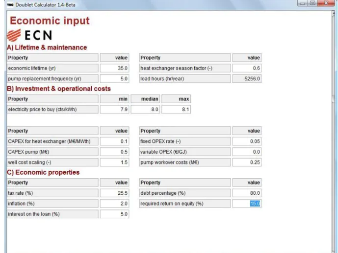
Once opened, the model presents the user with an input screen. On this screen nearly all variables are presented and can be altered if desired. Default values are present in the input screen, which correspond to certain general conditions or scenarios in the Netherlands. The units of each variable are shown in brackets next to the name. Several things will be highlighted from the input screen displayed below.

Because many variables, such as permeability and reservoir thickness, are not known to great certainty before the wells are drilled, these are represented by uncertainty curves. A minimum, median and maximum value is needed for these variables, which are then interpreted as triangular distributions.

The number of simulation runs in the top left corner refers to the number of times that the scenario is processed. For each run, a single value from each of the triangular distributions is chosen and used to calculate the UTC for that run. The results of each run are then aggregated and presented as a distribution in the output section. More runs will result in a more detailed and accurate final curve.

(25)

Fewer runs means the calculations are finished more quickly and this setting is useful if the user is on a slow computer.

In Figures 4.4 below, the input screen is shown. It is one whole screen, with the lower sections reached by scrolling down:

(26)

(27)

Figure 4.4 a, b, and c: Collectively, the input screen of DoubletCalc (Heat version).

These three figures show the input screen. The first describes the geological conditions of the targeted reservoir, the second the technical details needed to drill there, and the third the economic conditions of the project.

When all the fields have been adapted to the user’s satisfaction, the user should press “Calculate!” and the system will start processing. Should any input variables have been improperly entered, such as a negative permeability or if the minimum and maximum of a distribution don’t make sense, an error message will appear. If everything runs smoothly, an extra window with the output screen appears.

(28)

(29)

On the left, the input values are repeated, so that the user knows where these figures came from. On the right, the geotechnical and economic outputs are shown. The key output is the UTC, but other output values are also displayed, such as the total CAPEX, the total expenditures over time and subcomponents of those such as the annual loan payment.

Both the geotechnical and economic section have additional buttons labelled “Time Series Plots” and “Stochastic Plots”. These buttons lead to graphs which display, respectively, the time dependent variables varying over time and the Monte Carlo plots for time independent variables.

Time dependent variables such as Interest part of the Loan Payment. This graph represents the annual cost of debt over all the Monte Carlo iterations. The five lines stand for the range of possibilities depending on circumstances. Minimum and maximum designate the most extreme scenarios, and P10, P50 and P90 stand for the likelihood that the interest part of the loan payment is over that value out of a hundred. The interest is less every consecutive year as more of the principal has been paid off by that time, reducing the interest. The graph is negative, representing the fact that the owner loses less money over time to interest payments.

Figure 4.6 The interest payment per year, one of the output graphs of DoubletCalc.

The discounted yearly expenses, seen in the Figure below, represent the outflow of cash due to operation and maintenance costs. The sharp peaks every five years are due to the replacement of the ESP, which is a necessary but relatively expensive operation. The frequency and cost are among the adaptable input variables.

(30)

Figure 4.7 The yearly expenses payment, one of the output graphs of DoubletCalc.

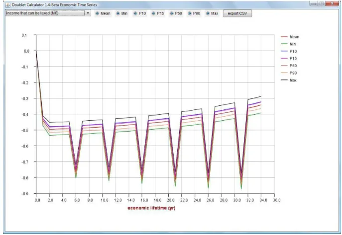
The taxable income is the sum of several outgoing cash flows, including the operational costs, depreciation of the plant, and the interest part of the payment. These are considered business expenses, and thus taxed under Dutch business tax law, since it is assumed that businesses making profits in one part of their operation invest those profits in other parts of their company. Again, the sharp peaks of the pump replacement are clearly seen in this curve. Because this is looked at as income, the values are all negative since they are outgoing cash flows.

(31)

Figure 4.8 The taxable income of the project, one of the output graphs of DoubletCalc. Note that the y-axis is negative.

The taxes paid yearly are simply a function of the taxable income and the tax rate. It is a positive amount because, under Dutch tax law, it is effectively added to the yearly income (a negative amount), from a different, profitable unit of the company.

(32)

Figure 4.9: The yearly paid taxes is also an output graph of DoubletCalc.

(33)

Figure 4.10: The Net Income after taxes, another output graph of DoubletCalc.

This is useful for an exploiter who needs to know what the annual cashflows will look like. A summation graph, with all of the above, is also available.

Some variables are not time dependent, or are aggregate results over the lifetime of the project. Such time independent variables are shown as a Monte Carlo (MC) curve, which displays the values resulting from each MC simulation, such as the predicted initial capital investment shown below.

(34)

Figure 4.11: This is a probability distribution of the total investment, one of the available graphs in DoubletCalc.

P90, P50 and P10 refer to the chance that the given value is above that number. So a P90 of 6.63 M€ means that there is a 90% chance the initial capital investment is above 6.63 M€.

Also shown are the expected cumulative discounted total expenses, not including capital expenditures.

(35)

Figure 4.12: A probability distribution of the cumulative discounted total income.

(36)

Figure 4.13: A probability distribution of the Unit Technical Cost, another output screen available on DoubletCalc.

This project is thus 50% likely to result in a UTC of at least 10.65 €/GJ. The 90% guarantee, often required by investors, for this project is a UTC of 13.18 €/GJ, which is relatively expensive. For comparison’s sake, the ECN SDE+ reference scenario for heat production results in a UTC 10.65 €/GJ.

4.3.2 Heat and Electricity Model

An adaptation of the original model also allows for the (co-)production of electricity by using a factor to divide the primary energy to heat and electricity purposes. For this model, the input screens are slightly different, including the primary energy divisor, separate load hours for electricity and heat production, and additional capital investment costs.

(37)

Figure 4.14a and b: Together, the input screen of the CHP version of DoubletCalc.

As a demonstration, the input values shown above were used for this project. Taking a generic project at 3000 m depth, a regular geothermal gradient and with a 50%/50% primary energy division, the following results are yielded:

(38)

Figure 4.15a and b: Together, part of the Output screen of the CHP version of DoubletCalc.

The output values above were produced. Note that the UTC for heat is quite low at a P50 of 7.70 €/GJ, while the UTC for electricity is remarkably high at a P50 of 30.4 €ct/kWh. Also curious is the

(39)

very high P10 of 5.97€/kWh. This is because, at this temperature, production of electricity is not efficient at all, and parasitic demand from the pumps is relatively high. It would not be

recommended to start a CHP geothermal project at such a location.

Figure 4.16: The summary screen of variables changeable over time, available in DoubletCalc.

The graph above shows the variation over time of the time-dependent variables. Yearly costs are higher than the geothermal heat project and pump replacement costs play a proportionally smaller role than in the Heat only model.

4.3.3 Factors affecting cost

One of the research sub-questions addresses which factors have the most significant influence on costs. This can be determined from the model, by creating a so-called Spider Diagram. For this diagram, a base case is chosen and the UTC calculated of that situation. Next, several main variables are each individually modified to determine the effect of that mutation on the UTC. These results are then collated in Excel and graphically represented, giving a clear visual indication of which variables have the most significant effect on the UTC.

This was done for a heat-only plant with the following base case variables:

Variable Value Permeability (mad) 500 Depth (m) 2000 Return T (degrees C) 30 Temperature Gradient (C/m) 0,031

Well Cost Scaling (-) 1,5

Lifetime (yr) 30

(40)

Interest rate (%) 5

Load Hours 5256

Table 4.2: the basic settings of a hypothetical project tested in DoubletCalc.

The base case UTC was 7.23 €/GJ. The resulting Spider Diagram is the Figure below:

Figure 4.17: A Spider diagram showing the effect of certain variables on the UTC for a hypothetical project.

The variable with the greatest effect on UTC is the temperature gradient, followed by the depth. Intriguingly, both of these are geological variables, implying that accurate knowledge of the reservoir conditions is critical for an accurate budget proposal. The next three most influential variables are the load hours, the return temperature and the permeability. The latter of these is another geological variable, and the former two are technical. Economic variables such as interest rate and debt percentage are actually of relatively little influence on the UTC.

4.3.4 Effect of Government policy

There are three government policies examined: the effect of a lump sum subsidy such as the MEI, the effect of paying the premium for a government guarantee of the project, and the effect of the additional cost of a blowout preventer and hydrocarbon separator. Taken in isolation, the effects of these policies are roughly analysed by modification of the investment costs, as shown in the Figure below. These effects are calculated relative to a project with the default conditions of the CHP model, except that the permeability is set to 200 Dm, with only the depth changing as per the y-axis.

0 5 10 15 20 25 30 0,4 0,6 0,8 1 1,2 1,4 1,6 Unit Tec h n ic al Co st [e u ro /GJ ]

Fraction of standard value

Spider Diagram Unit Technical Cost

Permeability (mD) Depth (m)

Return T (degrees C)

Temperature Gradient (C/m) Well Cost Scaling (-)

Lifetime (yr)

Debt Percentage (%) Interest rate (%) Load Hours

(41)

Figure 4.18 Effects on UTC of isolated policies.

These policies, in isolation have the most effect when depth is small, as investment costs are also relatively low. The effect of a lump sum subsidy is quite noticeable on the UTC, reducing it by at least 0.6€/GJ for this project. However, compared with the SDE+, which would effectively reduce the UTC to the correction rate, the lump sum cannot be seen as the preferred option.

The effect of the premium is quite small, although private insurance may be more expensive. This UTC increase ranges from 0.06€/GJ for the deepest to 0.60€/GJ for the shallowest project. This needs to be weighed against a possible payout of 85% of the investment to a maximum of only 7.2M€. It will be up to individual developers to decide. The effect of the premium is quite small, especially if the SDE+ is allowed to take effect.

The BOP and hydrocarbon separator are additional costs that are prudent regardless of government policy, given the troubles experienced at some current projects. The UTC does rise with these

additional investments, but this ranges from about 0.25€/GJ to 1.50€/GJ from deepest to shallowest. Given that the deeper projects are more attractive anyway; this may not be a significant setback. 4.3.5 Results with distance effects

Drilling of the wells is generally performed in a deviated fashion, so that the two wellheads are adjacent and there is no significant need for overland pipelines. At the aquifer level, the wells are significantly further apart. In this model, that distance is kept to at least 1700m to avoid thermal breakthrough during the economic lifetime of the project. Thermal breakthrough is when the cold water front from the injection well reaches the production well. Granted, this has been warmed somewhat by the surrounding rock, but it is usually the start of a precipitous decline in well productivity.

A small modification of the CHP model allows a look at the consequence of drilling directly vertical and using a pipeline to connect the two well heads.

-4000 -3500 -3000 -2500 -2000 -1500 -1000 4 9 14 19 D e p th UTC [euro/GJ]