Portland State University
PDXScholar
Dissertations and Theses Dissertations and Theses
Spring 5-17-2016
Tree Graphs and Orthogonal Spanning Tree Decompositions
James Raymond Mahoney
Portland State University
Let us know how access to this document benefits you.
Follow this and additional works at:http://pdxscholar.library.pdx.edu/open_access_etds Part of theMathematics Commons
This Dissertation is brought to you for free and open access. It has been accepted for inclusion in Dissertations and Theses by an authorized Recommended Citation
Mahoney, James Raymond, "Tree Graphs and Orthogonal Spanning Tree Decompositions" (2016).Dissertations and Theses.Paper 2944.
Tree Graphs and
Orthogonal Spanning Tree Decompositions
by
James Raymond Mahoney
A dissertation submitted in partial fulfillment of the requirements for the degree of
Doctor of Philosophy in
Mathematical Sciences
Dissertation Committee: John Caughman, Chair
Nirupama Bulusu Derek Garton Paul Latiolais Joyce O’Halloran
Portland State University 2016
c
2016 James Raymond Mahoney
This work is licensed under a
Abstract
Given a graph G, we construct T(G), called thetree graph of G. The vertices of T(G) are the spanning trees ofG, with edges between vertices when their respective spanning trees differ only by a single edge. In this paper we detail many new results concerning tree graphs, involving topics such as clique decomposition, planarity, and automorphism groups. We also investigate and present a number of new results on orthogonal tree decompositions of complete graphs.
Dedication
This dissertation is dedicated to Brigette, who cheerfully humors me whenever I inevitably start speaking math to her. Also to my family, whose support and encour-agement have helped me focus and go further in my education than I ever thought possible.
Acknowledgements
First and foremost I need to thank John Caughman for all of his time and effort as my adviser during my years at Portland State. John introduced me to graph theory and took a chance by becoming my Master’s adviser without knowing much about me. His tireless dedication to all of his students is remarkable. John’s suggestions for topics of inquiry and methods of attack made much of this work possible, while his keen editing eye greatly improved the quality of its presentation. I cannot thank you enough.
Thank you to the rest of my committee members for believing that my work was worthwhile.
Thank you to the math department at Portland State University for providing me with the Enneking Fellowship for two years. This generous support allowed me to spend my academic hours researching instead of teaching.
Thank you to all of my professors at Portland State University and the University of Portland for helping me realize and achieve my educational goals.
Thank you to Gary Gordon, who introduced me to matroid basis graphs and helped me discover the connection between my original research and tree graphs.
Thank you to Georgia Reh for assistance in editing this paper.
Lastly, thank you to Brendan McKay for the nauty program, to Ed Scheiner-man for his matgraph MATLAB package, and to the development group behind the Geometer’s Sketchpad software, all of which were critical to my visualization and understanding of tree graphs.
Table of Contents
Abstract i
Dedication ii
Acknowledgments iii
List of Figures vi
Glossary of Symbols viii
1 Introduction 1
1.1 Overview . . . 1
1.2 Organization . . . 2
2 Background 4 2.1 Graph Terminology . . . 4
2.2 Preliminary Results on Spanning Trees . . . 5
2.3 Tree Graphs . . . 6
3 The Tree Graph Function and Parameters 10 3.1 The Tree Graph Function . . . 10
3.2 Parameters of Tree Graphs . . . 21
4 Properties of Tree Graphs 28 4.1 Paths and Cycles . . . 28
4.2 Centers . . . 31
4.3 Local Properties . . . 34
4.4 Homomorphisms . . . 36
4.5 Automorphism Groups . . . 37
4.6 Induced Subgraphs and Planarity . . . 44
4.7 Clique Decomposition . . . 48
4.8 Special Families . . . 51
4.9 Conjectures . . . 58
5 Trees and Decompositions of Complete Graphs 68 5.1 Background and Terminology . . . 68
5.2 Literature . . . 76
5.3 New Results . . . 76
5.4 Conjectures . . . 79
Appendix A Selected Algorithms 84
Appendix B Examples of Graph Families 85
B.1 Grid Graphs . . . 85
B.2 Complete Multipartite Graphs . . . 85
B.3 Pn,k Graphs . . . 86 B.4 Prism Graphs . . . 86 B.5 θa,b,c Graphs . . . 87 B.6 Wheel Graphs . . . 87 B.7 J Graphs . . . 87 B.8 Named Graphs . . . 88
Appendix C Spectrum Data from T(Pn,2) 89
Appendix D Catalog of Tree Graph Data 91
List of Figures
Figure 1 Depictions of K5, P5, and C5 . . . 4
Figure 2 Showing the construction of T(C4) . . . 7
Figure 3 Showing the construction of T(K4−e) . . . 8
Figure 4 Isoparic graphs with isomorphic tree graphs . . . 13
Figure 5 The construction of a planar dual . . . 14
Figure 6 An example of dual spanning tree construction . . . 15
Figure 7 Dual spanning trees in the cube and octahedron graphs . . . . 16
Figure 8 Examples of wheel and Halin graphs . . . 17
Figure 9 Creating the tree graph of the vertex union of two graphs . . . 19
Figure 10 An example of the trimming process . . . 20
Figure 11 A proper four-coloring of T(K4−e) . . . 22
Figure 12 K4−e and the house graph . . . 24
Figure 13 A hamiltonian cycle through T(K4 −e) . . . 28
Figure 14 Hamiltonian cycles using and avoiding edge e0 in T(K4−e) . 29 Figure 15 Cycles of various lengths inT(K4−e) . . . 30
Figure 16 A hamiltonian path between vertices x and y inT(K4−e) . . 30
Figure 17 Various xy-paths in T(K4−e) . . . 30
Figure 18 Trees and their complements determine the center of T(G) . . 33
Figure 19 Common neighbor graphs in T(K4−e) . . . 36
Figure 20 An asymmetric graph G with |Aut(T(G))|= 12 . . . 38
Figure 21 Building a cycle that contains e and e0 . . . 39
Figure 22 A graph that fails to satisfy the conclusion of Theorem 4.15 . 42 Figure 23 The house graph showing deletion and contraction of an edge . 44 Figure 24 T(H) with the noted induced subgraphs shown . . . 46
Figure 25 Showing the tree graph of the diamond is nonplanar . . . 47
Figure 26 Showing the tree graph of the butterfly is nonplanar . . . 47
Figure 27 Clique decomposition of the tree graph of the diamond . . . . 50
Figure 28 The µ= 5 unicycles of the diamond . . . 51
Figure 29 Spanning tree of θ3,2,1 and corresponding edge in K3,2,1 . . . . 53
Figure 30 Constructing T(K3,2) from Q3 . . . 57
Figure 31 P3,2 and its tree graph . . . 61
Figure 32 The tree graph T(P4,2) . . . 62
Figure 33 Two bracelet graphs with regular tree graphs . . . 64
Figure 34 A regular graph that is not vertex-transitive . . . 65
Figure 35 Showing degree and partition type are not equivalent . . . 66
Figure 36 The 1-factorization GK8 . . . 68
Figure 37 Lengths and centers of edges in a rotational drawing of K8 . . 70
Figure 39 Starter graphs for the GK2n 1-factorization . . . 72
Figure 40 Starter graphs for the HK2n 1-factorization . . . 73
Figure 41 Distance and direction for edge pairs in a drawing of K8 . . . 74 Figure 42 Examples of opposing pair graphs . . . 74 Figure 43 Examples of rest graphs . . . 75 Figure 44 A successful test of the conjecture for K6 . . . 80
Glossary of Symbols
α(G) Independence number of graph G χ(G) Chromatic number of graphG δ(G) Minimum degree of graphG
∆(G) Maximum degree of graph G κ(G) Vertex connectivity of graph G κ0(G) Edge connectivity of graph G
µ(G) Number of spanning unicycles in graph G τ(G) Number of spanning trees of graph G
θa,b,c Theta graph
A(G) Adjacency matrix of graph G
Aut(G) Automorphism group of graph G C(G) Center of graph G
circ(G) Circumference of graph G Cn Cycle graph onn vertices
diam(G) Diameter of graphG
d(x, y) Distance between vertices
Dn Dihedral group with n elements
ecc(G) Eccentricity of graph G E(G) Edge set of graph G
f Number of faces in a given plane graph F 1-factorization ofK2n
g(G) Glory of graph G
G Complement of graph G
G±e Edge e added to/deleted from graph G G·e Edge e contracted in graph G
Kn Complete graph on n vertices
Kr1,r2,...,rk Complete multipartite graph
L(G) Line graph of graph G
m Number of edges of a given graph
MG Graphic matroid of graphG
n Number of vertices of a given graph
OP Gt(·) Opposing pair graph for K2n
Pn,k Graph joining two vertices withn openly-disjoint paths of lengthk
rad(G) Radius of graphG
Sn Symmetric group onn elements
SG(·) Starter graph for K2n T(G) Tree graph of graph G
v(G) Equal to m−n+ 1 in graphG V(G) Vertex set of graph G
Wn Wheel graph on n vertices
Zn Cyclic group on n elements
∼ Adjacency a b Binomial coefficient | | Cardinality
Cartesian product of graphs
× Cartesian product, direct product
∩ Intersection
∼
v Minor ≤ Subgraph, subgroup ⊆ Subset ∆ Symmetric difference ∪ Union J
1 Introduction
1.1 Overview
Given a graph G, we can construct a new graph T(G), called the tree graph of G. The vertices ofT(G) are the spanning trees of G. We place an edge between vertices
x and y in T(G) when their respective spanning trees differ only by a single edge. Tree graphs have been studied since at least 1966, when Cummins [4] wrote an in-fluential paper defining tree graphs and showing that they are hamiltonian. Although this original paper was published in an IEEE engineering journal, graph theorists soon took interest in the objects and additional papers found their way into mathematics journals. Some were motivated to study tree graphs because of their possible use as topologies for networks [26].
The first wave of tree graph results emerged from the late 1960s through the mid 1970s. These papers continued to investigate properties of tree graphs relating to hamiltonicity [10, 13] as well as the connection between tree graphs and the broader category of mathematical objects called matroid basis graphs [20, 21].
Interest in tree graphs was renewed by additional papers published from the late 1980s through the early 2000s. This second wave of research concerned itself with graph properties such as connectivity [1, 16] and chromatic number [26]. Variants of tree graphs were also considered during this time [24, 25].
While many papers about tree graphs have been published over the last half-century, there is still much that remains to be considered, including many classic graph parameters, such as the clique number and independence number. Other standard graph theoretic concepts such as planarity, decomposition, and regularity, as well as more algebraic topics, like automorphism groups, vertex-transitivity, and integrality, are likewise ripe for exploration.
When a new mathematical object is defined, many questions immediately arise. What properties does this object have? What is the relationship between this object and other known objects? In this way, research into tree graphs is similar to research into line graphs. Given a graph G, there is a deterministic construction (given in Section 4.8) one can follow to produce its line graph, L(G). Line graphs have been defined since at least the early 1930s, and have proven to be a very fruitful area of graph-theoretic research. We can answer questions about relationships between properties of a graph and properties of its line graph. We can predict the structure of line graphs and determine when a graph is a line graph. These same lines of inquiry can be extended to tree graphs, and, as mentioned earlier, many important questions are still open.
This dissertation aims to make a significant contribution to the study of tree graphs by filling in many of the missing pieces in our understanding of these objects. We have several novel results and many conjectures that are likely to lead to further proofs. For example, we have discovered a structural property of tree graphs that may lead toward a characterization, based on their relationship to matroid basis graphs. We have also found an infinite family of integral tree graphs, which is of importance to graph theory even outside of the realm of tree graphs. This research will help paint a more accurate picture of an object that has already been given considerable, and well-deserved, attention.
1.2 Organization
Chapter 2 provides a background on spanning trees and tree graphs, with definitions, examples, and preliminary results. The heart of this paper is broken down into three main explorations: Chapter 3 will look at the tree graph construction as a function
from the set of graphs to itself. Here we consider questions of injectivity, surjectivity, fixed points, and other functional properties. We also investigate relationships found between graphs and their tree graphs. Specifically, in what ways can we relate pa-rameters of graphs to papa-rameters of their tree graphs? In Chapter 4 we will consider tree graphs as a family and describe properties that they all share. We will attempt to provide a classification of tree graphs, and discuss special classes, such as regular tree graphs. In Chapter 5, we investigate spanning tree decompositions of complete graphs. In particular, we explore the Brualdi-Hollingsworth conjecture which states that every 1-factorization ofK2nhas a full set ofndisjoint orthogonal spanning trees.
Appendix A contains some of the algorithms used in the course of this research. In Appendix B we illustrate many of the common graph families which appear in this paper. Appendix C is a collection of spectrum data for a particular family of tree graphs. Appendix D is a partial catalog of data collected on tree graphs generated for this research, while Appendix E contains data relevant to specific 1-factorizations from the last chapter. Each chapter will contain relevant previous work from the literature as well as novel results. Many conjectures and open problems will be given as well.
2 Background
2.1 Graph Terminology
A graph G= (V, E) is a set V of vertices together with a multiset E of edges, which is made up of unordered pairs of vertices from V. Edges are said to connect vertices, and if two vertices x and y are connected by an edge they are said to be adjacent, which we denote by x ∼y. We can also refer to the edgexy. The degree of a vertex is the number of edges incident to it. If there is an edge from a vertex to itself, that edge is called aloop. If there are no repeated edges or loops in E,Gis called asimple graph. Unless stated otherwise, all graphs discussed in this paper will be assumed to be simple and have a finite number of vertices.
The complete graph Kn has n vertices, all of which are adjacent to each other.
Complete graphs are also called cliques. A 3-clique is sometimes called a triangle. Complete multipartite graphs, such as Ka,band Ka,b,c, partition their vertices into the
sizes given by their subscripts, where two vertices are adjacent if and only if they are in different cells of the partition. A path of length n is an alternating sequence of vertices and edges v1, e1, v2, e2, . . . , vn, en, vn+1 such that each edgeei joins vi and
vi+1 and no two vertices are the same. A cycle of length n is a path of length n, but where the first and last vertices are the same. Cycles must contain at least three edges. Figure 1 shows examples of some of these graphs.
A graph with no cycles is called a forest. If there is a path between every pair of vertices in a graph, the graph is said to be connected. A tree is a connected forest. The vertices of degree one in a graph are called pendant vertices, and the pendant vertices in a tree are called leaves. A subgraph H = (V0, E0) of a graph G is any graph where V0 ⊆ V and E0 ⊆ E. This relation is denoted byH ≤G. A maximally connected subgraph of a graph is called acomponent. A vertex (edge) whose deletion from a graph increases the number of components is called a cut vertex (cut edge). A graph is said to be k-connected if at least k vertices need to be removed in order to disconnect it. The complete graph Kn is said to be k-connected for all k < n.
A spanning tree of a connected graphG is a subgraph that contains all of the same vertices as G and is a tree.
Two graphs G and H are isomorphic, written G ∼= H, if they have exactly the same structure. Specifically, graphs are shown to be isomorphic by finding a bijection between their vertices that preserves the adjacency relationship, i.e., an isomorphism. Throughout Chapter 2, we assume graphs are connected unless otherwise stated. In general, we will reserve the parametersm =|E(G)|andn =|V(G)|for the number of edges and vertices, respectively, in a graph.
2.2 Preliminary Results on Spanning Trees
The following elementary results will be used repeatedly in later sections of the paper.
Lemma 2.1. [32, Theorem 2.1.4] Every spanning tree of a graph withn vertices has
n−1 edges.
Lemma 2.3. [32, Propositions 2.1.6-7] If T and T0 are spanning trees of a graph G
and e∈E(T)−E(T0), then there is an edge e0 ∈E(T0)−E(T) such that T −e+e0
and T +e0−e are both spanning trees of G.
Lemma 2.4. For any spanning tree T of a graph G and any edge e ∈ E(G), there exists an edge e0 ∈E(T) such that T +e−e0 is a spanning tree of G.
Proof. If e ∈E(T), let e0 =e. Otherwise, adding e to T produces exactly one cycle (see Corollary 2.1.5.b in [32]). Remove any other edgee0 of that cycle to get back to a spanning tree.
Lemma 2.5. Every edge in a graph G is contained in some spanning tree of G.
Proof. Let e ∈ E(G) and T be a spanning tree of G that does not contain e. Then by Lemma 2.4, T +e−e0 is a spanning tree ofG for some edge e0 ∈T.
Lemma 2.6. Every acyclic subgraph of a graph Gis contained in some spanning tree of G.
Proof. Let H ≤ G be acyclic, and T be a spanning tree for G that minimizes t = |E(H)−E(T)|. If t = 0, choose T. Now suppose t 6= 0. Pick e ∈ E(H)−E(T). Then T +e has a cycleC. Since H is acyclic, there exists e0 ∈ E(C)−E(H). Then
T +e−e0 is a spanning tree that contradicts the minimality of t. Therefore t = 0 and such a spanning tree exists.
2.3 Tree Graphs
Graphs are used as an abstract model of relationships between objects, where vertices represent the objects and edges denote relationships between them. In a tree graph T(G), the vertices represent all of the spanning trees of G and the edge relationship
describes how near the spanning trees are to each other, in terms of their edge sets. In later sections of this paper, we will often simultaneously treat such a vertex both as a vertex of T(G) and as a spanning tree of G. When there is no room for confusion, we will sometimes refer to spanning trees simply as trees. Note also that in this paper, every graph that will be used to construct a tree graph will be assumed to be connected. This restriction will be explained at the end of Section 3.1.
Given a graph G, its tree graph T(G) is constructed in the following way. The vertices of T(G) are all of the spanning trees of G. Two distinct spanning trees are adjacent inT(G) if we can get from one to the other by swapping a single edge. This is called the edge exchange property. More formally, two trees are adjacent if the size of the symmetric difference of their edge sets is two.
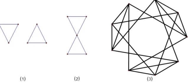
Let us look at this construction for the four-cycle C4 in Figure 2.
Figure 2: Showing the construction of T(C4)
First in (1) we see C4. Then in (2) we see the four spanning trees of C4 with dashed edges. In (3), we view these four trees as four vertices in a graph with the edge exchange condition for adjacency. Denote the four edges of C4 by the names T, R, B, and L, for top, right, bottom, and left, respectively. Let us consider which trees the upper left tree should be adjacent to. We can take out L and replace it by R to create the top right tree. We can swap U for R to get the bottom left tree. We can also exchange B for R to get the bottom right tree. In this way, the top left
tree is adjacent to every other tree in T(C4), so we see the bold edges connecting them. The same is true for every tree in the graph. Thus in (4) we see that the tree graph of the four-cycle is the complete graph on four vertices, or using graph notation, T(C4)∼=K4.
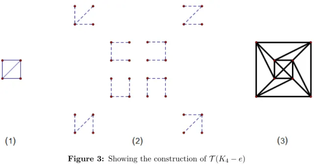
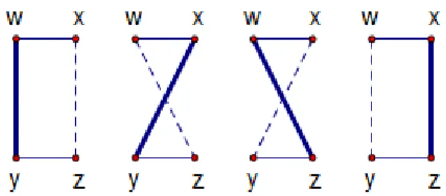
Let us consider one more example. This time we will add another edge to C4 to get K4−e. Figure 3 shows its tree graph construction. In (1) we see K4−e. Next in (2) using dashed edges we see its eight spanning trees. The new diagonal edge has given us four more trees to play with. Finally, in (3) in bold we see T(K4−e). By adding one edge to our starting graph we have picked up four more vertices and twelve more edges in the tree graph.
Figure 3: Showing the construction of T(K4−e)
Note that our spanning trees are considered different if they have different sets of edges, not solely if they are nonisomorphic. So while K4 −e has two isomorphism classes of trees, P3 and K1,3, it has eight distinctly labeled trees. These are what we are interested in comparing.
examples of tree graphs. Multiple parameters were measured, recorded, and compared to existing data for patterns. The production and analysis of such a data set is a distinguishing feature of this work, and a sizable catalog is included in Appendix D to aid in future investigations.
3 The Tree Graph Function and Parameters
Often when a new graph is constructed from an old one, properties of the new graph can be inferred from properties of the old. These properties may be parametric or structural. For example, the number of vertices in the line graph L(G) of G is the number of edges in G. This is a parametric relation, since we are describing a graph parameter in terms of other known values. We also know that a vertex of degreek in
G leads to a k-clique inL(G); this is a structural relation.
We can think of the tree graph construction as a process where we input a graph and get its tree graph as output. This section contains results relating properties of graphs to properties of their tree graphs. Throughout Chapter 3, we assume graphs are connected unless otherwise stated.
3.1 The Tree Graph Function
Following an edge in a tree graph T(G) amounts to changing one spanning tree of
G into another using the edge exchange property. One might wonder, then, if it is always possible to transform one tree into any other by iteration of this process. The following result shows us that this is the case.
Lemma 3.1. The tree graph T(G) is connected for all graphs G.
Proof. Let T and T0 be two trees of G. Using Lemma 2.3 repeatedly, we can add edges from E(T0)−E(T) while removing edges from E(T)−E(T0) until we have swapped in all of the missing edges. This induces a path from T toT0 inT(G). Thus there is a path between every two vertices inT(G), so it is connected.
The distance between vertices x and y in a graph G is the minimum number of edges in a path from x to y, and is denoted by d(x, y). Distance between vertices in
T(G) depends on how similar the corresponding trees are, which we measure by how many edges they have in common. More formally, we have the following.
Lemma 3.2. For trees T1 and T2 in T(G),
d(T1, T2) =n−1− |E(T1)∩E(T2)|=|E(T1)∆E(T2)|/2
where ∆denotes the symmetric difference of sets.
Proof. Every tree has n−1 edges. To get from T1 toT2, we have to swap the edges that they do not share, of which there aren−1− |E(T1)∩E(T2)|. The set of swapped edges occur in pairs in the symmetric difference. Repeated use of Lemma 2.3 swaps these pairs, reducing t=|E(T1)∆E(T2)| to zero in t/2 steps.
The eccentricity of a vertex x, written ecc(x), is defined by
ecc(x) = max{d(x, y) | y∈V(G)}
and represents the farthest away that a vertex can be from x. The minimum eccen-tricity over all vertices of a graph is called theradius, denoted rad(G). The maximum eccentricity is called thediameter, denoted diam(G). The collection of all vertices of minimum eccentricity is called the center of G, and is denoted by C(G).
If two trees have no edges in common, by Lemma 3.2 they would be at distance
n−1. On the other hand, we have at mostm−(n−1) =m−n+ 1 available edges to swap in order to change between two trees. Thus we have the following result.
Lemma 3.3. For any graph G,
In general we cannot say much about the relationship between the diameters of
G and T(G). For example, consider G ∼= Kn. The diameter of complete graphs is
1, whereas once n ≥4, we can always find two spanning trees that have no edges in common, making the diameter for the tree graphs at least n−1. Thus these values can be arbitrarily far apart.
We can view the tree graph operation as a function from the set of connected graphs, G, to itself, i.e. T : G → G. We can thus investigate properties of this function, such as surjectivity, injectivity, pre-images, and fixed points.
Theorem 3.4. [13, Lemma 1] For any graph G that contains a cycle, T(G)∼= G if and only if G∼=K3.
This tells us that the only nontrivial fixed point of the tree graph function is the triangle. We trivially have that T(K1)∼=K1.
Theorem 3.5. [13, Lemma 2] For any n >3, the cycle graph Cn is not a tree graph.
Roughly, this result says that tree graphs contain much more structure than a simple cycle. It also tells us that the tree graph function is not surjective.
Theorem 3.6. [13, Theorem 1] Let G be a graph that contains a cycle. The graphs in the iterated tree graph sequence
G,T(G),T(T(G)), . . .
will continue to get larger, either in number of edges or vertices or both, unless G∼=
K3.
Lemma 3.7. The tree graph of a tree is a single vertex.
Proof. The only spanning tree of a treeT is the tree T itself, so in this case, the tree graph will be K1.
Lemma 3.8. For any n≥3,T(Cn)∼=Kn.
Proof. The cycle Cn has n vertices and n edges. Thus diam(T(Cn))≤1 by Lemma
3.3. The diameter cannot be zero, since T(Cn) has n ≥ 3 vertices by Lemma 3.6.
Thus the diameter is one. The only graphs with n > 1 vertices and diameter 1 are the complete graphs onn vertices. Therefore T(Cn)∼=Kn.
We saw an example of this in the first tree graph construction in Figure 2 of Section 2.3 when we discovered that T(C4)∼=K4.
We say that two graphs are isoparic if they have the same number of vertices and edges, but are not isomorphic.
Theorem 3.9. The tree graph function is not injective.
Proof. This means us that two nonisomorphic graphs can have the same tree graph. Figure 4 shows an example of two isoparic graphs that have isomorphic tree graphs with 55 vertices and 277 edges. Corollary 3.16 will give a trivial way to break the injectivity of this function, so the importance of this particular counterexample comes from the fact that the two isoparic graphs are 2-connected.
The property of being isoparic is not a necessary or sufficient condition for two graphs to have isomorphic tree graphs. For example, both K3,3 and K1,1,4 have six vertices and nine edges. However, the tree graph of the former has 81 vertices, while the tree graph of the latter has 48. Theorem 3.10 will show another general case where nonisomorphic graphs have the same tree graph.
A graph is planar if it can be drawn in the plane with no edge crossings. A plane graph is a particular drawing of a planar graph in the plane that contains no edge crossings. There may be many different ways to draw a planar graph as a plane graph. In a plane graph, afaceis a simply connected region of the plane bounded by at least three edges. For a more complete introduction to these topics, see Chapter 6 in [32]. By convention, G∗ denotes the planar dual ofG. The dual relationship for planar graphs exchanges the roles of vertices and faces. In particular, G∗ is constructed by putting a vertex for every face in a plane graph G, including the infinite outer face. Vertices are connected by an edge each time their corresponding faces share a boundary edge. If G has m edges, n vertices, and f faces, G∗ will have m edges, f
vertices, andn faces. Figure 5 illustrates the construction of a planar dual. We begin with a plane graph G in (1). In (2) we see the new vertices added for each face of
G, and the new edges connecting vertices if their respective faces share a boundary edge. Finally in (3) we see the planar dualG∗ redrawn by itself.
Theorem 3.10. If G is 3-connected and planar, then T(G)∼=T(G∗).
Proof. A classic theorem of Whitney [34] says that if G is 3-connected and planar, then G∗ is unique up to isomorphism and simple (moreover, also 3-connected and planar). Thus T(G∗) is well-defined in this case.
A result [18, p. 37] shows that there is a natural bijection between the spanning trees ofGand the spanning trees ofG∗. ThusT(G) andT(G∗) have the same number of vertices. The construction of the bijection [18, p.258] implies that the adjacency relationship between the spanning trees is preserved. That is,Ti ∼Tj inT(G) if and
only if Ti∗ ∼Tj∗ in T(G∗). Therefore T(G)∼=T(G∗).
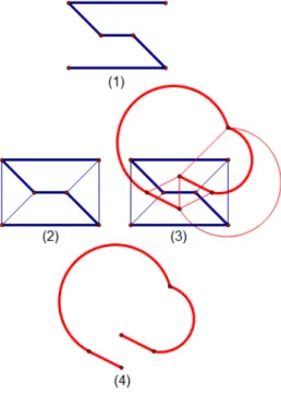
Figure 6 shows an example of this bijection. In (1) we see the starting spanning tree T of a graph G. In (2) we see T in bold along with the rest of G. Next in (3) we see the planar dual G∗ drawn in, with the new edges that cross the edges in
E(G)−E(T) in bold. Finally in (4) we see the dual tree T∗.
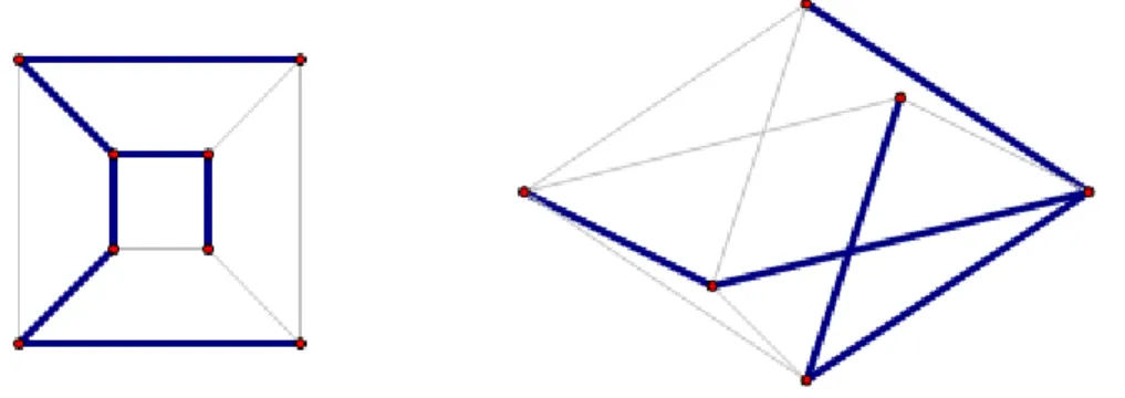
The cube, with six faces and eight vertices, is the planar dual of the octahedron, with eight faces and six vertices. Figure 7 shows an example of dual spanning trees in these planar dual graphs. The tree graph of these graphs is too large to show here, having 384 vertices and 3768 edges.
Figure 7: Dual spanning trees (bold edges) in the cube and octahedron graphs
Some examples of 3-connected planar graphs are polyhedral graphs, such as the previously mentioned cube and octahedron, and Halin graphs. To construct a Halin graph, start with a planar drawing of a tree with at least one vertex of degree at least three and no vertices of degree two. Then draw a cycle through all of the leaves in a way that keeps the graph planar. The wheel graphWnis a special type of Halin graph
where the base tree is a star graph, which is a tree with n−1 leaves. The following result shows us another situation where nonisomorphic graphs can have isomorphic tree graphs.
Corollary 3.11. For any non-wheel Halin graph H, we have H H∗ but T(H) ∼= T(H∗).
Proof. Euler’s formula (see page 241 in [32]) says that for any plane graph,n−m+f = 2. Suppose G and G∗ are isomorphic. Then n = f, which by Euler gives us that
n −m +n = 2, so m = 2(n −1). Let H be a Halin graph and TH the spanning
since the edges ofH either come from the set ofn−1 edges inTH or from thel-cycle
through its leaves. For H∗ to be isomorphic to H, we would need l =n−1, so that |E(H)|=n−1 +n−1 = 2(n−1). But a tree with n−1 leaves is a star, soH would be a wheel graph. Thus if H ∼=H∗, H is a wheel graph. In either case, by Theorem 3.10, T(H)∼=T(H∗).
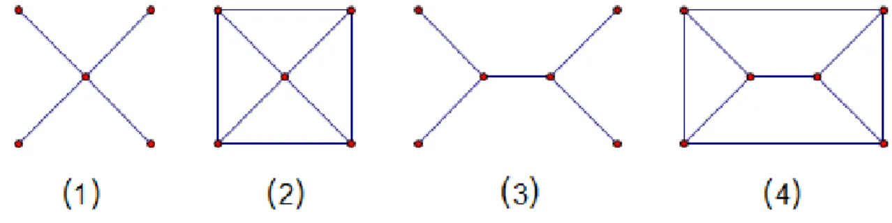
Figure 8 shows (1) a star graph, (2) the wheel graph W5, (3) a non-star tree, and (4) the Halin graph built from the tree.
Figure 8: Examples of wheel and Halin graphs
The last three results together tell us that, given a tree graph T(G), it may not be possible to find a unique graph G that generates it. One step in that direction comes from Lemma 1.2 in [21], which says that if the spanning trees corresponding to any vertex and all of its neighbors in T(G) are given, the remaining spanning trees can uniquely be assigned to the vertices of T(G). From this information a unique
G can be recovered by taking the union of all of the spanning trees. In general, reconstruction seems to be a challenging problem. That is, given a tree graphT(G), we want to find a graph H such that T(H)∼=T(G). One ambitious desire would be to determine under which circumstances this is possible, and moreover when it is, to know when H is unique.
Let GJ
xyH be the graph that identifies the vertex x of G with the vertex y of
V(G)×V(H), and two vertices (x, x0) and (y, y0) are adjacent if and only if either
x =y and x0 ∼y0, or x0 =y0 and x ∼ y. The following result shows us that certain tree graphs can be built up as products of smaller tree graphs.
Theorem 3.12. For any graphs G and H, and vertices x∈V(G), y ∈V(H),
T(GK
xy
H)∼=T(G)T(H).
Proof. Let cbe the vertex of GJ
xyH where Gand H are joined at x and y. Then
c is a cut vertex of GJ
xyH. As such, every spanning tree of G J
H has at least two edges incident toc: at least one each fromG andH. Thus each tree of GJ
xyH
can be broken down into a spanning tree of Gand a spanning tree of H. Conversely, every pair of spanning trees from G and H, when joined at c, make a spanning tree for GJ
xyH. Thus T(G J
xyH) and T(G)T(H) have the same vertex set.
Let T1 ∼ T2 in T(G)T(H). This is (x, y) ∼ (x0, y0) for x, x0 ∈ T(G) and
y, y0 ∈ T(H). By the adjacency rules, WOLOG x = x0 and y ∼ y0 in T(H). This tells us that y and y0 have the edge exchange property. Consider the graphs xJ
y
andx0J
y0. Sincex=x0, these two graphs differ only by a single edge. Thus they are adjacent inT(GJ
xyH). Using the same argument we can see that adjacent vertices
inT(GJ
xyH) will have their corresponding vertices inT(G)T(H) be adjacent as
well. Therefore adjacency is the same in both graphs and they are isomorphic. We also have the following corollary, which implies that it does not matter which vertices we choose to identify in the process described above.
Corollary 3.13. For any u, x∈V(G) and v, y∈V(H),
T(GK
uv
H)∼=T(GK
xy
Thus from now on we will simply write GJ
H without any reference to the vertices being identified.
Theorem 3.12 was proved independently in [2] (see Lemma 1). The smallest nontrivial example of this is the graph constructed by letting two triangles share a vertex, as shown in Figure 9. In (1) we see two copies ofK3. We then see them joined at a vertex in (2). Finally in (3) we see the tree graph of the middle graph, which is the Cartesian product T(K3)T(K3)∼=K3K3, since T(K3)∼=K3 by Lemma 3.8.
Figure 9: Creating the tree graph of the vertex union of two graphs
Using similar reasoning and a simple induction argument, we get the following two corollaries.
Corollary 3.14. Fix anyk ≥1and let Gbe the disjoint union of graphsH1, . . . , Hk.
Then T(G)∼=T(H1). . .T(Hk).
Corollary 3.15. Fix any k ≥ 1 and graphs H1, . . . , Hk. Let G ∼= H1J· · ·JHk.
Then T(G)∼=T(H1). . .T(Hk).
LetG−e denote the graph where the edgee is deleted andG·e denote the graph where the edge has been contracted. When an edge is contracted, its endpoints are
identified and we follow the convention that the newly formed loop edge is deleted so that simple graphs remain loopless.
For any graph G, let S = {e ∈ E(G) | e is a cut edge}. Define Gtrim to be the graph remaining after contracting all of the edges in S. If we think of G as being a collection of smaller graphs joined together with theJ
operator, we are removing all of the component graphs that are trees. These are the pieces that do not contribute anything new to the tree graph, since they are in every tree. This brings us to our next corollary.
Corollary 3.16. For any graph G, T(Gtrim)∼=T(G).
Proof. SupposeG∼=G1JGt, whereG1 is 2-connected andGtis a tree. By Theorem
3.12, T(G)∼=T(G1)T(Gt). By Lemma 3.7,T(Gt) is a single vertex. It is trivial to
show that HK1 ∼=H for any graph H. Thus T(G)∼=T(G1). Using Corollary 3.15 we can then conclude that T(Gtrim)∼=T(G).
Figure 10 shows a graph G on the left andGtrim on the right.
Figure 10: An example of the trimming process
Corollary 3.14 allows us to restrict our attention to the case of connected graphs, as is our working assumption in this chapter. Since connected graphs without cut vertices are 2-connected, Corollary 3.15 allows us to restrict further to consider only the tree graphs of 2-connected graphs. Indeed, the tree graphs of 2-connected graphs are the building blocks of all tree graphs, just as primes are the building blocks of the natural numbers. Accordingly, every time a graph is mentioned as being the input for
the tree graph function in this paper, we will henceforth assume that it is 2-connected unless otherwise noted.
3.2 Parameters of Tree Graphs
In this section we collect results concerning parameters of tree graphsT(G), especially in their relation to the parameters of G.
Recall that κ(G) is the vertex connectivity of a graph: for a non-complete graph, the minimum number of vertices needed to be removed in order to disconnect it. Likewise, κ0(G) is the edge connectivity. For more information on these parameters, see Chapter 4 in [32]. The smallest degree of a graph is δ(G). A classic result is that the following chain of inequalities holds [33]:
κ(G)≤κ0(G)≤δ(G).
One way to get a feel for these inequalities is that deleting all of the neighbors of a vertex or all of the edges incident to a vertex will separate that vertex from the rest of the graph. Additionally, deleting an edge from a graph does not delete its incident vertices in the way that deleting a vertex also removes its incident edges. The following theorem of Liu highlights a special property of tree graphs.
Theorem 3.17. [16, Corollary 2.8] For all graphs G,
κ(T(G)) =κ0(T(G)) =δ(T(G)).
This theorem tells us that tree graphs are maximally connected. This can be an important property to network designers, as local disruptions should not jeopardize the entire structure.
Acoloring of a graph is an assignment of numbers to its vertices. Aproper coloring is a coloring where adjacent vertices get different numbers. The chromatic number of a graph, χ(G), is the minimum number of colors in a proper coloring of G. See Chapter 5 in [32] for more information on this parameter.
The following result gives us an upper bound on the chromatic number of a tree graph based on the number of edges of the underlying graph.
Theorem 3.18. [26, Theorem 1] For all graphs G,
χ(T(G))≤ |E(G)|.
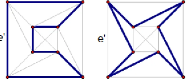
As an example, K4−e has five edges, so the tree graphT(K4−e) needs at most five colors for a proper coloring. It contains a K4 subgraph, so requires at least four colors. Figure 11 demonstrates that this is sufficient.
Figure 11: A proper four-coloring of T(K4−e)
The girth of a graph, denoted girth(G), is the length of its shortest cycle. The circumference of a graph, denoted circ(G), is the length of it longest cycle. This next result gives us a lower bound on the smallest degree (δ) and an upper bound on the largest degree (∆) of a tree graph T(G) based on cycle and edge information from the underlying graph G.
Theorem 3.19. [17, Theorem 1] For a graph G with n vertices and m edges, let
v =m−n+ 1. Then
v·(girth(G)−1)≤δ(T(G))≤∆(T(G))≤v·(circ(G)−1).
In our K4−e example, we have m = 5 and n = 4, so v = 2. The length of the shortest cycle is three while the length of the longest cycle is four. Putting these together gives us that 4 ≤δ(T(K4−e)) and ∆(T(K4−e))≤ 6. Compare these to the actual values of δ(T(K4−e)) = 4 and ∆(T(K4−e)) = 5.
The chromatic index of a graph, χ0(G), is the edge coloring version of the chro-matic number. We need a minimum of ∆(G) distinct colors to properly color the edges of G. A famous theorem by Vizing [29] says that at most one more color is necessary. Together with Theorem 3.19, this gives us the following corollary.
Corollary 3.20. For a graphGwithn vertices and m edges, letv =m−n+ 1. Then
χ0(T(G))≤(circ(G)−1)·v+ 1.
If we know something about the structure of the trees, we can give an exact value to the minimum degree of the tree graph. A unicycle is a connected graph with exactly one cycle. All unicycles in this paper will be assumed to be spanning.
Theorem 3.21. For a graph G with n vertices and m edges, let v =m−n+ 1.
(i) There exists a tree of Gsuch that every unicycle that contains it has cycle length equal to girth(G) if and only if δ(T(G)) =v·(girth(G)−1).
(ii) There exists a tree ofGsuch that every unicycle that contains it has cycle length equal to circ(G) if and only if ∆(T(G)) = v·(circ(G)−1).
Proof. (i) Suppose first that such a tree existed. Then by Theorem 4.22 it will achieve degreev·(girth(G)−1), which by Theorem 3.19 is as small as possible. Thus
δ(T(G)) = v·(girth(G)−1).
Now suppose δ(T(G)) =v·(girth(G)−1). There is some vertex x inT(G) with that degree. Again by Theorem 4.22,xis part ofv cliques. Eachc−clique contributes
c−1 edges to the degree of x. Lets1, s2, . . . , sv be the number of edges added to the
degree ofx for each of the v cliques that contain x. Since each clique in T(G) comes from a cycle inG, the smallest a clique can be is the size of the smallest cycle, which is girth(G). Thussi ≥girth(G)−1. We have thats1+s2+· · ·+sv =v·(girth(G)−1),
so the average value of the si is (girth(G)−1). Since they are all positive integers
bounded by their average, they must equal that average. Thusxis only part of cliques of size girth(G), so all unicycles containing xhave cycle length equal to girth(G).
(ii) The proof is similar to that of (i).
The graph K4−e is an example that has such a tree for the lower bound. The value girth(K4 −e) = 3 and v = 5−4 + 1 = 2. Any tree that contains the diagonal edge cannot be part of a unicycle with cycle size 4. The only other possible cycle size is 3, so all unicycles containing that tree have cycle size 3. Thus in T(K4−e) we see four vertices of minimum degree 2·(3−1) = 4. The house graph, shown in Figure 12, has girth 3 and is a nonexample. The tree graph of the house graph has minimum degree 5, which is not a multiple of 2, which is the v value for the house. Therefore no tree of the house can contain only unicycles with cycle size 3.
It is easier to find graphs that meet the lower bound than the upper bound. The bound on ∆ is sharp for some families, such as the θa,2,2 and Pn,k graphs that are
defined in Section 4.8.
The clique number of a graph, ω(G), is the size of its maximum clique. We can place a lower bound on the clique number of a tree graph based on the circumference of the base graph.
Theorem 3.22. For any graph G,
ω(T(G))≥circ(G).
Proof. Let s = circ(G). The cycle Cs is then a subgraph of G. By Corollary 4.19, T(Cs) will be a subgraph of T(G). By Lemma 3.8, T(Cs) ∼= Ks. Thus T(G) will
contain a Ks subgraph, and so ω(T(G)) is at least circ(G).
For most of the tree graphs studied, this bound is tight. However, for some families of graphs the gap between the two values can get arbitrarily large. For example, the
Kn,2 graphs have a circumference of 4. Call the vertices in the two-cell x and y. Consider the set of trees where x is adjacent to all of the vertices in the n-cell and
y is adjacent to just one of them. There are n such trees and they all differ by just one edge, so they will all be adjacent in T(Kn,2). Thus ω(T(Kn,2)) ≥ n, which can be taken as far away from 4 as we want.
Each vertex in a clique needs a different color in a proper coloring. This gives us the easy boundχ(G)≥ω(G). From this fact and Theorem 3.22 we get the following corollary.
Corollary 3.23. For any graph G,
χ(T(G))≥circ(G).
For almost all of the tree graphs studied, the clique number and the chromatic number were the same. One time where these differed was when the base graph was
K4. We have that ω(T(K4)) = 4<5 =χ(T(K4)). Figuring out exactly when these values coincide would be valuable.
A regular graph has vertices all of the same degree. The independence number of a graph is α(G), defined to be the maximum number of vertices in a graph that induce a subgraph with no edges. Let G have n vertices and m edges. Let µ(G) be the number of spanning unicycles inG, and letv =m−n+ 1. LetPn,k be the graph
where two vertices are joined byn openly-disjoint paths of lengthk, n, k >1. Paths are openly-disjoint if and only if they share only their endpoints.
In the proof for Theorem 3.22 we saw that each unicycle with cycle size c in G
gives rise to ac−clique inT(G). Later on, Theorem 4.22 will show us that T(G) can be decomposed intoµ(G) cliques such that each vertex is part of exactlyv cliques. At most one vertex from each of those cliques can be chosen to be part of an independent set. Thus, choosing a vertex prevents one from choosing any other vertices from the
v cliques it is part of. So the number of cliques in a decomposition divided by the number of cliques per vertex should give us an upper bound on the number of independent vertices we can choose. That brings us to our next result.
Theorem 3.24. For a graph Gwithn vertices andm edges, let v =m−n+ 1. Then
α(T(G))≤ bµ(G)/vc.
Proof. Let S = {s1, s2, . . . , sα} be the vertices in a maximum independent set in T(G). We count the ordered pairs of the form (si, ci), where ci is a clique in the
clique decomposition from Theorem 4.22 that contains si. If we choose the vertices
first, we haveα choices. Each vertex is inv cliques, so we have that many choices for
ci. Thus we haveα·v ordered pairs. Suppose that α·v > µ(G). Since we only have
µ(G) different cliques, by the pigeonhole principle at least one of them is repeated in our set of ordered pairs. That implies that we have chosen at least two vertices from the same clique, which contradicts the fact that the vertices are chosen from an independent set. Thus we have thatα·v ≤µ(G). Since the independence number is an integer, we get the final bound of α(T(G))≤ bµ(G)/vc.
For example, if the base graph is K1,1,3, we have µ= 18 and v = 3, while b183c= 6 ≥ 5 = α. For another, let G = P3,2, which is 6-regular. Then we have µ = 6 and
v = 2, which gives the correct value of α = 3. If T(G) is regular, this bound seems to be tight.
4 Properties of Tree Graphs
This section will contain results concerning structural properties that all tree graphs share. Some concern graph-theoretic properties, while others are more algebraic in nature. Together they help demonstrate how truly remarkable the family of tree graphs is. Throughout Chapter 4, we assume graphs are connected unless otherwise stated.
4.1 Paths and Cycles
A graph is hamiltonian if it has a cycle that contains all of its vertices. When we investigate this property for tree graphs, we are really looking into whether or not it is possible to cycle through all of the spanning trees of a graph by just swapping one edge at a time. The following result, from the first paper on tree graphs, says this is always possible.
Theorem 4.1. [4, Theorem L] For any graph G, T(G) is hamiltonian.
Figure 13 shows one possible hamiltonian cycle through T(K4−e). The hamil-tonicity of tree graphs might be desirable to circuit or network designers who need to test the performance of every possible spanning tree of their system. Some authors, such as that of [11], even came up with constructive algorithms to generate and cycle through all of the spanning trees of a graph in this way.
A graph is uniformly hamiltonian if for each of its edges e, there exists a hamil-tonian cycle that uses e and one that avoids e.
Theorem 4.2. [10, Corollary 2] For any graph G, the tree graph T(G) is uniformly hamiltonian.
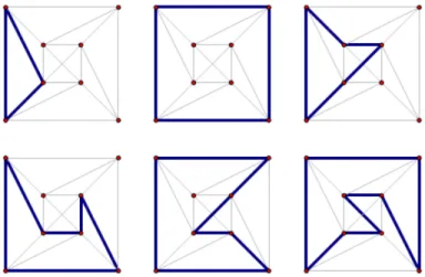
So whileK4−e is hamiltonian, it is not uniformly hamiltonian, as no hamiltonian cycle can use the diagonal edge. This result gives us that T(K4 −e), however, is uniformly hamiltonian. Figure 14 shows an example of this for one edge, e0.
Figure 14: Hamiltonian cycles using and avoiding edge e0 inT(K4−e)
A graph is edge-pancyclic if each of its edges is used in a cycle of every possible size from its girth to its circumference. Hamiltonian-connected means that there is a hamiltonian path between every two vertices in the graph. Path-full implies that if there exists paths of length m and n between two vertices, then for all m < k < n
there exists a path of length k between them as well.
Theorem 4.3. [1, Theorems 3.1-3] T(G) is edge-pancyclic, hamiltonian-connected, and path-full for any graph G.
Figure 15: Cycles of various lengths in T(K4−e)
Figure 16: A hamiltonian path between vertices xand y inT(K4−e)
Figure 17: Variousxy-paths inT(K4−e)
Together these results show us that tree graphs are very structured and have plenty of edges with which to move through the graph.
4.2 Centers
A subgraphH = (V0, E0) ofG= (V, E) is aninduced subgraph if for every two vertices
x and y in V0, x ∼ y in H if and only if x ∼ y in G. In general, the complement
Gc has the same vertices as G but with x ∼ y in Gc if and only if x y in G. For our purposes, we need a second type of complement. Specifically, if H ≤G, then we define H = (V(H), E(G)−E(H)). In particular, the complement of a spanning tree
T of Gwill be understood to be the complement of T in G.
Recall that the center of a graph, denoted C(G), is the subgraph induced on the set of vertices of minimum eccentricity. In some sense, these are the vertices that are closest to all other vertices. If G ∼= C(G), we say that G is self-centered. An equivalent definition is to say that rad(G) = diam(G). Some tree graphs are self-centered while others have a proper center. The distinction between the two cases is explored in the next results.
Lemma 4.4. Let T be a spanning tree of G. If T is acyclic, then the eccentricity of the vertex in T(G) corresponding toT is given by
ecc(T) =m−n+ 1.
Proof. Every tree has n−1 edges, so T has m−n+ 1 edges. By Lemma 2.6, T is contained in a spanning tree of G. Lemma 3.2 tells us this tree will be at distance
m−n+ 1 fromT, which by Lemma 3.3 is the maximum possible.
Corollary 4.5. If all trees of G have acyclic complements, T(G) is self-centered.
Proof. By Lemma 4.4 all of the trees will correspond to vertices in T(G) with the same eccentricity, which implies rad(T(G)) = diam(T(G)) and that T(G) is self-centered.
Since all cycles have at least three edges, if v =m−n+ 1 = 2 no tree complement can contain a cycle. Thus all graphs with v = 2 have self-centered tree graphs. This family includes the Pn,k graphs and the θa,b,c graphs, described later in this chapter.
A graph isbipartite if its vertices can be partitioned into two sets such that every edge in the graph has one end in each set. Bipartite graphs have no odd cycles. Thus ifGis bipartite andv = 3,T(G) will be self-centered. In general, we get the following corollary.
Corollary 4.6. Let G be any graph, and let v = m−n+ 1. If v < girth(G), then T(G) will be self-centered.
The converse of this corollary is false. Consider the graph G = K4,1,1. Since it has only two vertices of degree higher than two, every cycle in it contains at least one vertex of degree two. Suppose the complement of a spanning tree T of G contained a cycle. The complement T would then contain all of the edges incident with at least one of the degree two vertices. Thus in T that vertex would have no edges incident to it, contradicting the fact that T is a spanning tree. Therefore all trees of
Ghave acyclic complements, and so by Corollary 4.5 the graphT(G) is self-centered. However, we have that girth(G) = 3 and v(G) = 4.
As the inverse to Lemma 4.4, we have the following.
Lemma 4.7. LetT be a spanning tree ofG. IfT contains a cycle, then the eccentricity of the vertex in T(G) corresponding to T satisfies
ecc(T)< m−n+ 1.
Proof. No tree inT(G) contains T, since it contains a cycle. This implies d(T0, T)< m−n+ 1 for all T0 ∈ T(G), since no tree can be m−n+ 1 away from T by using
all of the edges in its complement. Thus ecc(T)< m−n+ 1.
Combining the last few results, we can now describe the trees in the center of a non-self-centered graph.
Theorem 4.8. If T(G) is not self-centered and T ∈ C(T(G)), then T contains a cycle.
Proof. Since the center is proper, not all trees in T(G) have the same eccentricity. Thus by Corollary 4.5 at least one tree T0 has a complement that contains a cycle. No tree with an acyclic complement can be in the center, since by Lemmas 4.4 and 4.7 its eccentricity would be strictly greater than that of T0. Thus all trees in the center have a complement that contain a cycle.
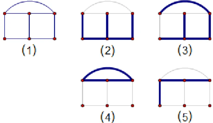
Figure 18 shows an example of the previous results on tree graph centers. In (1) we see our graphG. It has 6 vertices and 8 edges, and sov = 3. In (2) and (3) we see trees T1 and T2 in bold. Note that (4) shows T1, which contains a triangle. On the other hand, (5) shows T2, which is acyclic. Thus trees can be at most distance two from T1 and distance three from T2 in T(G). Since there is only one triangle in G and that is the only cycle that can be formed with v = 3 edges, T1 is the only vertex in the center of T(G).
The converse of Theorem 4.8 is also not true. Consider G = K5. The center of
T(G) consists of the five spanning trees that are star graphs. Let T be any path through G. The complement T contains a triangle between the two endpoints of the path and the middle vertex of the path. Therefore T contains a cycle, but T is not in the center of T(G).
The next result, from the literature, relates the diameter of self-centered graphs with the diameter of their line graphs. A graph is d-self-centered if it is self-centered with diameter d. We define Grida,b to be the graph PaPb.
Theorem 4.9. [28, Theorem 2.2] Let G and L(G) be d- and f-self-centered graphs, respectively. Then f ∈ {d−1, d, d+ 1}.
Thus if a graph and its line graph are both self-centered, their diameters can differ by at most one. A noteworthy passage in [28] poses the following:
If G = K2 (1-self-centered) then L(G) = K1 is 0-self-centered. On the other hand, examples ofGandL(G) which are bothd-self-centered can be easily found. Hence we have the following interesting problem: Determine the remaining (if any)d-self-centered graphs whose line graphs are(d−1) -or (d+ 1)-self-centered.
Several tree graphs are examples of the latter type. The tree graphs ofK3,2, K4,2, and Grid3,2 all have line graphs that are also self-centered whose diameter has in-creased by one. We conjecture that there is an infinite family of tree graphs with this property, but it has not been fully investigated yet.
4.3 Local Properties
An ordered pair (E,B) is a matroid if E is a set of elements and B ⊆ P(E) is a set of subsets of E called bases satisfying: (i) IfB ∈ B then B 6=∅and (ii) IfA, B ∈ B
then for all a ∈ A−B there exists b ∈ B −A such that (A− {a})∪ {b} ∈ B. It turns out that the spanning trees of a graph can be used to form a matroid. If we letE be the set of edges of a graphG, and B be the set of spanning trees ofG, then
MG = (E,B) is a matroid.
Given any matroidM, the matroid basis graph is the graph whose vertices are the bases of the matroid and where two vertices are adjacent if and only if their bases differ by a single element. Notice that this sounds remarkably like our definition of a tree graph. In fact, when the collection of spanning trees of a graph is viewed as a matroid as above, tree graphs can be seen as a special case of matroid basis graphs. Thus results that hold for matroid basis graphs also apply to tree graphs.
Tree graphs constitute a proper subclass of the class of all matroid basis graphs, however. For example, let M = {{1,2,3,4},{12,13,14,23,24,34}}. The matroid basis graph for M is the octahedron (see Figure 7). Since the bases all have two elements, if they were the edges of a tree, the base graph would need to have exactly three vertices. But our edge set has four elements. Indeed, there are no simple graphs with three vertices and four edges. Thus, this matroid basis graph is not a tree graph. Maurer published influential papers [20, 21] that described and characterized ma-troid basis graphs. Many local and global properties were investigated. One concept in these papers is that of the common neighbor graph, defined as follows. Let x and
y be vertices of G that are at distance two. Let N ={v ∈V | v ∼ x, v ∼ y} be the set of common neighbors of x and y. The common neighbor graph of x and y is the subgraph of G induced on the set of vertices N ∪ {x, y}. A square is the graph C4 and thepyramid is the wheel graphW5.
Theorem 4.10. All common neighbor graphs of tree graphs are squares or pyramids.
some graph. Thus the set of spanning trees of a connected graph together with the set of edges of the graph is a graphic matroid. A remark in [21, p. 125] states that every graphic matroid is binary (another designation for matroids, whose definition is not important for our purposes), which, in turn, is equivalent to the basis graph having no induced octahedra (see Theorem 4.1 in [21]). Thus T(G), as the basis graph for the set of spanning trees ofG, contains no induced octahedra. But Lemma 1.4 in [20] says that the common neighbor graph of a basis graph is either a square, pyramid, or an octahedron. Since we just learned that octahedra are ruled out for tree graphs, all common neighbor graphs of tree graphs are either squares or pyramids. Additionally, Corollary 4.3 in [21] states that if G is not a Cartesian product of complete graphs, then T(G) contains at least one common neighbor graph that is a pyramid.
Figure 19 shows square and pyramid common neighbor graphs in T(K4−e).
Figure 19: Common neighbor graphs inT(K4−e)
4.4 Homomorphisms
A homomorphism from graph G to H is a function φ : V(G) → V(H) such that
x ∼ y ⇒ φ(x) ∼ φ(y). If there is a homomorphism from G to H, we will write
G → H. Homomorphisms preserve some of the structure of the original graph. In this section we make a short investigation of how the tree graph function interacts with graph homomorphisms.
A natural first question about homomorphisms is to determine when a homo-morphism can exist between graphs. One necessary condition for G → H is that
χ(G)≤χ(H). In any proper coloring, distinctly colored vertices cannot be adjacent, so H cannot require fewer colors than G needs. From this observation we get the following result.
Theorem 4.11. The assumption that G→H does not imply T(G)→ T(H).
Proof. By way of a counterexample, notice that there is a homomorphism fromK4−e to K3 that maps the two vertices of degree 2 to a single vertex of K3 and the two vertices of degree 3 to the two other vertices in K3. However, χ(T(K4 −e)) = 4, while χ(T(K3)) = 3, so there can be no homomorphism from T(K4−e) to T(K3). Therefore G→H does not imply T(G)→ T(H).
4.5 Automorphism Groups
We denote by Aut(G) the the group of automorphisms of G, which is the group of permutations of V(G) that respect adjacency in G. The glory g(G) of a graph G is the size of its automorphism group, so that g(G) = |Aut(G)|. (This definition gives us a way to quantify how glorious a graph is!) Automorphism groups can range in size anywhere from the full symmetric group Sn (of order n!) for complete graphs, all the
way down to the trivial group (of order 1) for some graphs. Such inglorious graphs are called asymmetric. It is known that, asymptotically, almost all finite graphs are asymmetric (see Corollary 2.3.3 in [9]).
The data gathered for this research indicate that tree graphs tend to be very glorious. This high level of symmetry can arise even if the base graph is asymmetric. For example, the smallest 2-connected asymmetric graph can be visualized (see Figure 20) by identifying an edge of two squares and adding a diagonal edge through one of
the squares. We will refer to this graph as Asym6. Its tree graph has 29 vertices and 122 edges, and has an automorphism group of order 12. In fact, the automorphism group is isomorphic to D12, the symmetries of a regular hexagon.
Figure 20: An asymmetric graph Gwith|Aut(T(G))|= 12
Brendan McCay’s well-known computer program nauty [22] was used to find the glories of the tree graphs constructed during this research. In some smaller cases, the automorphism group itself could be uncovered. The number of groups discerned so far is perhaps not large enough to support any serious conjecture, but all of the groups found have either been dihedral groups or (products of) symmetric groups. This only applies to graphs that are 2-connected but not 3-connected, a distinction that will be explained in Conjecture 4.33.
The two major results in this section relate the automorphism group of a tree graphT(G) to the automorphism group ofG. In Theorem 4.15 we see that the latter is always isomorphic to a subgroup of the former. In Theorem 4.16 we learn that in most cases, if G is sufficiently connected then the two groups are the same. We first prove several lemmas. We remind the reader of Menger’s theorem [23] on connectivity which says that if Ghas connectivity κ, then any two verticesx, y will be connected by at leastκopenly-disjointxy-paths (xy-paths are openly-disjoint if and only if they share only their endpoints xand y).
Lemma 4.12. Let G be a 2-connected graph and let e, e0 ∈E(G) be distinct. There is a cycle in G containing both e and e0.
Proof. By the fact thatG is 2-connected, we have thatκ≥2. Suppose that e and e0
a path from y toz openly-disjoint from the path yxz. The union of these two paths then creates a cycle containing e and e0.
Suppose now thate={w, x}and e0 ={y, z} share no vertices. Since the graph is connected, there exists a pathpfromwtoy. This path falls into one of several cases.
• the path pcontains neither xnor z: by Menger’s theorem there exists a path q
fromx to z openly-disjoint from p.
• the path p contains x but not z: by Menger’s theorem there exists a path q
fromw to z openly-disjoint fromp.
• the path p contains z but not x: by Menger’s theorem there exists a path q
fromx to y openly-disjoint fromp.
• the pathpcontains xand z: by Menger’s theorem there exists a pathq fromw
toy openly-disjoint from p.
In each case, the union ofp, q, e, ande0 produces a cycle containing the two desired edges.
Figure 21 illustrates each of the four cases. The bold edges represent the path p
and the dashed edges represent the path q.
Figure 21: Building a cycle that contains eande0
Lemma 4.13. Let G be a 2-connected graph and let e, e0 ∈E(G) be distinct. There exists a spanning tree of G which includes e and avoids e0.
Proof. By Lemma 4.12, there exists a cycle containing both e and e0. Start building a tree by first adding in all of the edges in that cycle except for e0. That collection of edges forms an acyclic subgraph of G. By Lemma 2.6, there is a tree that contains that subgraph. Thus we have a tree that contains e and does not containe0.
Let σ ∈ Aut(G). Then σ is a permutation of V(G) such that σ(x) ∼ σ(y) if and only if x ∼ y. But σ also induces a permutation ˆσ of edges of G. We define ˆ
σ :P(E(G))→ P(E(G)) to be the map satisfying
ˆ
σ(S) ={{σ(x), σ(y)} | {x, y} ∈S}.
We will view T, a spanning tree ofG, both as a vertex of T(G) and as a set of edges of G, depending on our need. By the adjacency restriction of σ on V(G), we know that ˆσ(T) ∼= T as a spanning tree. The function σ also induces an automorphism
φσ ∈Aut(T(G)) by φσ(T) = ˆσ(T).
There are two types of edges: those that are not contained in cycles (so-called cut edges) and those that are (so-called cycle edges). Since automorphisms preserve the structure of the graph, the edge orbits under Aut(G) are partitioned by these types. That is, cycle edges get sent only to cycle edges and cut edges get sent only to cut edges under the action of Aut(G).
Lemma 4.14. Let σ ∈ Aut(G) and φσ be defined as above. If φσ(T) = T for all
T ∈V(T(G)), then σˆ(e) =e for all cycle edges e∈E(G).
Proof. This theorem says that if an induced automorphism acts like the identity on T(G), then its base automorphism fixes cycle edges inG. We argue by contrapositive. Suppose that ˆσ does not fix all cycle edges in G. Then there exist distinct cycle edges e and e0 such that ˆσ(e) = e0. By Lemma 4.13, there exists a spanning tree T
of G that contains e and avoids e0. Then φσ(T)6=T, since ˆσ(T) contains e0 while T
does not. Therefore the statement is true by contrapositive.
Theorem 4.15. For any 2-connected graph G, there exists a subgroup
H ≤Aut(T(G)) such that Aut(G)∼=H.
Proof. Using the same notation as above, define Ψ : Aut(G)→Aut(T(G)) by Ψ(σ) =
φσ for any σ∈Aut(G). We claim that Ψ is a group homomorphism. To see this, let
σ1, σ2 ∈Aut(G) and T ∈V(T(G)). Then
Ψ(σ2◦σ1)(T) = φσ2◦σ1(T)
= ˆσ2(ˆσ1(T))
=φσ2(φσ1(T))
= Ψ(σ2)◦Ψ(σ1)(T).
Thus Ψ is a homomorphism. We will now show that Ψ is an injection. Let i be the appropriate identity automorphism. If Ψ(σ) = Ψ(i) then for any T ∈V(T(G)),
ˆ
σ(T) = φσ(T) = Ψ(σ)(T) = Ψ(i)(T) =φi(T) = ˆi(T).
This implies that ˆσ equals ˆi when they are acting on V(T(G)). But we want to show that σ equals i as elements of Aut(G), ie. when they are acting on V(G).
We are assuming that φσ(T) = T for all T ∈ V(T(G)). Since G is 2-connected,
every edge is a cycle edge. By Lemma 4.14, this means that ˆσ(e) = efor alle∈E(G). Thus ˆσ fixes all of the edges of G.
By way of contradiction, then, suppose σ does not fix all of the vertices in G, that is, σ(x) =y, for some x =6 y. If {w, x} is an edge that contains x, then either
ˆ
σ({w, x}) = {σ(w), y} is a different edge, which is a contradiction, or elsew=y and
σ(y) = x. Since G is 2-connected, it contains more than just the one edge {x, y} with endpoint x. Indeed, let {x, z} denote another edge in G. The transposition of
x and y forces z to move as well, which sends {x, z} to a different edge. This is a contradiction.
Thus we have that σ fixes all of the vertices of G, meaning σ = i. This implies that Ψ is an injective group homomorphism from Aut(G) into Aut(T(G)), which lets us conclude that the image of Aut(G) is the desired subgroup H.
As an example,
Aut(K4−e)∼=V4 ≤D8 ∼= Aut(T(K4−e))
where V4 is the Klein 4-group and D8 is the dihedral group of symmetries of the square. Note that this result might not hold if G is not 2-connected. For example, letGbe the star graph on five vertices with an edge added between two of the leaves; see Figure 22. The automorphism σ of G that swaps the two leaves 1 and 2 has the same effect on all of G’s trees as the identity automorphism i; ˆσ(T) = ˆi(T) for all
T ∈ V(T(G)). However, σ(1) = 2 = 1 =6 i(1) when acting on V(G), so σ 6= i in Aut(G).
In general, suppose two isomorphic trees are connected to a graph Gat the same vertex. Let G0 be this new graph. Let γ be the automorphism of G0 that swaps the two trees and fixes everything else. Then ˆγ(T) =T for all T ∈V(T(G0)), sinceG is fixed by γ. We then have that ˆγ = ˆibut γ 6=i. In this case Ψ would not be injective, which is what we want.
One way to prevent this issue is to assume that G is 2-connected, and thus has no cut edges. Since that is our running assumption in this paper, we do not include that hypothesis in the theorem.
If G contains a cycle, the result depends on whether or not G has any non-identity automorphisms that fix all of its cycle edges. For example, K3JK3 is not 2-connected, but none of its seven nonidentity automorphisms fix all of its cycle edges. Thus the theorem holds for it.
Theorem 4.16. Suppose G is 3-connected with m edges and n vertices. Then Aut(T(G))∼= Aut(G), except that ifm= 2(n−1), it is also possible thatAut(T(G))∼= Aut(G)×Z2.
Proof. The cycle automorphism group,Autc(G) is defined as the group of all functions
φ :E(G)→ E(G) such that X ⊆ E(G) is a cycle if and only ifφ(X) is a cycle. On page 329 of [31] we have that ifGis 3-connected, then Aut(G)∼=Autc(G). LetMG=
(E,B) be the graphic matroid of G. On the same page we are told that Aut(MG)∼=
Autc(G) for any graph. Corollary 3.5 from [21] gives us that Aut(T(G))∼= Aut(MG),
except that if m = 2(n −1), it is also possible that Aut(T(G)) ∼= Aut(MG)×Z2. Following the chain of isomorphisms gives us our result.
As an example of this result, K5 is 3-connected, and
An example of the exception is K4, with four vertices and six edges. Indeed,
Aut(T(K4))∼=S4 ×Z2 ∼= Aut(K4)×Z2.
A negative exception is K4,3. It is 3-connected and has seven vertices and twelve edges, yet
g(K4,3) =g(T(K4,3)) = 144.
4.6 Induced Subgraphs and Planarity
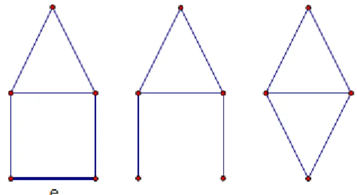
Recall thatG−eis the graph where the edgee is deleted andG·eis the graph where the edge has been contracted. Let us use the example of the house graph H and let
e be its bottom edge. Figure 23 shows H on the left with edge e in bold, H−e in the middle, and H·e on the right. The graph H−e is a triangle with two pendant vertices, which we know from Corollary 3.16 will have the same tree graph as K3. The graph H·e is the same as K4−e, and we saw what its tree graph looks like in Section 2.
Figure 23: The house graph showing deletion and contraction of an edge
In this section we learn that tree graphs contain the tree graphs of smaller graphs inside of them. We can use this knowledge to show that essentially all tree graphs