Multidimensional Scaling
Patrick J.F. Groenen
∗Michel van de Velden
†April 6, 2004
Econometric Institute Report EI 2004-15
Abstract
Multidimensional scaling is a statistical technique to visualize dissimi-larity data. In multidimensional scaling, objects are represented as points in a usually two dimensional space, such that the distances between the points match the observed dissimilarities as closely as possible. Here, we discuss what kind of data can be used for multidimensional scaling, what the essence of the technique is, how to choose the dimensionality, trans-formations of the dissimilarities, and some pitfalls to watch out for when using multidimensional scaling.
1
Introduction
Multidimensional scaling is a statistical technique originating in psychometrics. The data used for multidimensional scaling (MDS) are dissimilarities between pairs of objects. The main objective of MDS is to represent these dissimilarities as distances between points in a low dimensional space such that the distances correspond as closely as possible to the dissimilarities.
Let us introduce the method by means of a small example. Ekman (1954) collected data to study the perception of 14 different colors. Every pair of colors was judged by a respondent from having ‘no similarity’ to being ‘identical’. The obtained scores can be scaled in such a way that identical colors are denoted by 0, and completely different colors by 1. The averages of these dissimilarity scores over the 31 respondents are presented in Table 1. Starting from wavelength 434, the colors range from bluish-purple, blue, green, yellow, to red. Note that the dissimilarities are symmetric: the extent to which colors with wavelengths 490 and 584 are the same is equal to that of colors 584 and 490. Therefore, it suffices to only present the lower triangular part of the data in Table 1. Also, the diagonal is not of interest in MDS because the distance of an object with itself is necessarily zero.
∗Econometric Institute, Erasmus University Rotterdam, P.O. Box 1738, 3000 DR
Rotter-dam, The Netherlands (e-mail: [email protected])
†Department of Marketing and Marketing Research, Groningen University, P.O. Box 800,
Table 1: Dissimilarities of colors with wavelengths from 434 to 674 nm (Ekman, 1954). nm 434 445 465 472 490 504 537 555 584 600 610 628 651 674 434 – 445 .14 – 465 .58 .50 – 472 .58 .56 .19 – 490 .82 .78 .53 .46 – 504 .94 .91 .83 .75 .39 – 537 .93 .93 .90 .90 .69 .38 – 555 .96 .93 .92 .91 .74 .55 .27 – 584 .98 .98 .98 .98 .93 .86 .78 .67 – 600 .93 .96 .99 .99 .98 .92 .86 .81 .42 – 610 .91 .93 .98 1.00 .98 .98 .95 .96 .63 .26 – 628 .88 .89 .99 .99 .99 .98 .98 .97 .73 .50 .24 – 651 .87 .87 .95 .98 .98 .98 .98 .98 .80 .59 .38 .15 – 674 .84 .86 .97 .96 1.00 .99 1.00 .98 .77 .72 .45 .32 .24 –
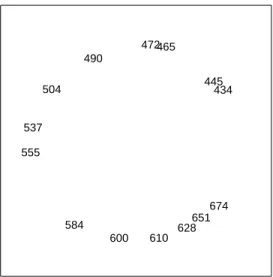
MDS tries to represent the dissimilarities in Table 1 in a map. Figure 1 presents such an MDS map in 2 dimensions. We see that the colors, denoted by their wavelengths, are represented in the shape of a circle. The interpretation of this map should be done in terms of the depicted inter-point distances. Note that, as distances do not change under rotation, a rotation of the plot does not affect the interpretation. Similarly, a translation of the solution (that is, a shift of all coordinates by a fixed value per dimension) does not change the distances either, nor does a reflection of one or both of the axes.
Figure 1 should be interpreted as follows. Colors that are located close to each other are perceived as being similar. For example, the colors with wavelengths 434 (violet) and 445 (indigo) or 628 and 651 (both red). In contrast, colors that are positioned far away from each other, such as 490 (green) and 610 (orange) indicate a large difference in perception. The circular form obtained in this example is in accordance with theory on the perception of colors.
Summarizing, MDS is a technique that translates a table of dissimilarities between pairs of objects into a map where distances between the points match the dissimilarities as well as possible. The use of MDS is not limited to psy-chology but has applications in a wide area of disciplines, such as sociology, economics, biology, chemistry, and archaeology. Often, it is used as a technique for exploring the data. In addition, it can be used as a technique for dimen-sion reduction. Sometimes, as in chemistry, the objective is to reconstruct a 3D model for large DNA-molecules for which only partial information of the distances between atoms is available.
434 445 465 472 490 504 537 555 584 600 610 628 651 674
Figure 1: MDS solution in 2 dimensions of the color data in Table 1.
2
Data for MDS
In the previous section, we introduced MDS as a method to describe relation-ships between objects on the basis of observed dissimilarities. However, instead of dissimilarities we often observe similarities between objects. Correlations, for example, can be interpreted as similarities. By converting the similarities into dissimilarities MDS can easily be applied to similarity data. There are several ways of transforming similarities into dissimilarities. For example, we may take one divided by the similarity or we can apply any monotone decreasing function that yields nonnegative values (dissimilarities cannot be negative). However, in Section 4, we shall see that by applying transformations in MDS, there is no need to transform similarities into dissimilarities. To indicate both similarity and dissimilarity data, we use the generic term proximities.
Data in MDS can be obtained in a variety of ways. We distinguish between the direct collection of proximities versus derived proximities. The color data of the previous section is an example of direct proximities. That is, the data arrives in the format of proximities. Often, this is not the case and our data does not consist of proximities between variables. However, by considering an appropriate measure, proximities can be derived from the original data. For example, consider the case where objects are rated on several variables. If the interest lies in representing the variables, we can calculate the correlation matrix as measure of similarity between the variables. MDS can be applied to describe the relationship between the variables on the basis of the derived proximities. Alternatively, if interest lies in the objects, Euclidean distances can be computed between the objects using the variables as dimensions. In this case, we use high dimensional Euclidean distances as dissimilarities and we can use MDS to reconstruct these distances in a low dimensional space.
Co-occurrence data are another source for obtaining dissimilarities. For such data, a respondent groups the objects into partitions and an n×n incidence matrix is derived where a one indicates that a pair of objects is in the same group and a zero indicates that they are in different groups. By considering the frequencies of objects being in the same or different groups and by applying special measures (such as the so-called Jaccard similarity measure), we obtain proximities. For a detailed discussion of various (dis)similarity measures, we refer to Gower and Legendre (1986).
3
Formalizing Multidimensional Scaling
To formalize MDS, we need some notation. Let n be the number of different objects and let the dissimilarity for objectsiand j be given byδij. The coor-dinates are gathered in ann×pmatrixX, wherepis the dimensionality of the solution to be specified in advance by the user. Thus, rowi from Xgives the coordinates for object i. Letdij(X) be the Euclidean distance between rows i andj ofXdefined as dij(X) = Ã p X s=1 (xis−xjs)2 !1/2 , (1)
that is, the length of the shortest line connecting pointsiandj. The objective of MDS is to find a matrixXsuch thatdij(X) matchesδij as closely as possible. This objective can be formulated in a variety of ways but here we use the definition of raw-Stressσ2(X), that is,
σ2(X) = n X i=2 i−1 X j=1 wij(δij−dij(X))2 (2)
by Kruskal (Kruskal, 1964a, 1964b) who was the first one to propose a formal measure for doing MDS. This measure is also referred to as the least-squares MDS model. Note that due to the symmetry of the dissimilarities and the distances, the summation only involves the pairs ij where i > j. Here, wij is a user defined weight that must be nonnegative. For example, many MDS programs implicitly choosewij = 0 for dissimilarities that are missing.
The minimization of σ2(X) is a rather complex problem that cannot be
solved in closed-form. Therefore, MDS programs use iterative numerical algo-rithms to find a matrixXfor whichσ2(X) is a minimum. One of the best
algo-rithms available is the SMACOF algorithm (De Leeuw, 1977, 1988; De Leeuw & Heiser, 1980; Borg & Groenen, 1997) based on iterative majorization. The SMACOF algorithm has been implemented in the SPSS procedure Proxscal (Meulman, Heiser, & SPSS, 1999). In Section 7, we give a brief illustration of the SMACOF algorithm.
Because Euclidean distances do not change under rotation, translation, and reflection, these operations may be freely applied to MDS solution without af-fecting the raw-Stress. Many MDS programs use this indeterminacy to center
the coordinates so that they sum to zero dimension wise. The freedom of rota-tion is often exploited to put the solurota-tion in so-called principal axis orientarota-tion. That is, the axis are rotated in such a way that the variance ofX is maximal along the first dimension, the second dimension is uncorrelated to the first and has again maximal variance, and so on.
Here, we have discussed the Stress measure for MDS. However, there are several other measures for doing MDS. In Section 8, we briefly discuss other popular definitions of Stress.
4
Transformations of the Data
So far, we have assumed that the dissimilarities are known. However, this is often not the case. Consider for example the situation in which the objects have been ranked. That is, the dissimilarities between the objects are not known, but their order is known. In such a case, we would like to assign numerical values to the proximities in such a way that these values exhibit the same rank order as the data. These numerical values are usually called disparities, d-hats, or pseudo distances, and they are denoted by db. The task of MDS now becomes to simultaneously obtain disparities and coordinates in such a way that the coordinates represent the disparities (and thus the original rank order of the data) as well as possible. This objective can be captured in minimizing a slight adaptation of raw Stress, that is,
σ2(db,X) = n X i=2 i−1 X j=1 wij(dbij−dij(X))2, (3)
over both the db and X, where bd is the vector containing dbij for all pairs. The process of finding the disparities is called optimal scaling and was first introduced by Kruskal (Kruskal, 1964a, 1964b). Optimal scaling aims to find a transformation of the data that fits as well as possible the distances in the MDS solution. To avoid the trivial optimal scaling solutionX=0anddbij = 0 for all
ij, we impose a length constraint on the disparities in such a way that the sum of squared d-hat’s equals a fixed constant. For example, Pni=2Pji−=11wijdb2ij =
n(n−1)/2 (De Leeuw, 1977).
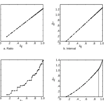
Transformations of the data are often used in MDS. Figure 2 shows a few examples of transformation plots for the color example. Let us look at some special cases.
Suppose that we choose dbij =δij for all ij. Then, minimizing (3) without the length constraint is exactly the same as minimizing (2). Minimizing (3)with the length constraint only changesdbij=aδij, whereais a scalar chosen in such a way that the length constraint is satisfied. This transformation is called a ratio transformation (Figure 2a). Note that, in this case, the relative differences ofaδij are the same as those forδij. Hence, the relative differences of thedij(X) in (2) and (3) are also the same. Ratio MDS can be seen as the most restrictive transformation in MDS.
dij .0 .2 .4 .6 .8 1.0 .0 .2 .4 .6 .8 1.0 1.2 δij ˆ dij .0 .2 .4 .6 .8 1.0 .0 .2 .4 .6 .8 1.0 1.2 δij ˆ dij .0 .2 .4 .6 .8 1.0 .0 .2 .4 .6 .8 1.0 1.2 δij ˆ dij .0 .2 .4 .6 .8 1.0 .0 δij ˆ .2 .4 .6 .8 1.0 1.2 1.4 a. Ratio b. Interval c. Ordinal d. Spline
Figure 2: Four transformations often used in MDS.
An obvious extension to the ratio transformation is obtained by allowing the dbij to be a linear transformation of the δij. That is, dbij = a+bδij, for some unknown values ofaandb. Figure 2b depicts an interval transformation. This transformation may be chosen if there is reason to believe that δij = 0 does not have any particular interpretation. An interval transformation that is almost horizontal reveals little about the data as different dissimilarities are transformed to similar disparities. In such a case, the constant term will domi-nate thedbij’s. On the other hand, a good interval transformation is obtained if the line is not horizontal and the constant term is reasonably small with respect to the rest.
For ordinal MDS, the dbij are only required to have the same rank order as δij. That is, if for two pairs of objects ij and kl we have δij ≤ δkl then the corresponding disparities must satisfydbij ≤dbkl. An example of an ordinal transformation in MDS is given in Figure 2c. Typically, an ordinal transforma-tion shows a step functransforma-tion. Similar to the case for interval transformatransforma-tions, it is not a good sign if the transformation plot shows a horizontal line. Moreover, if the transformation plot only exhibits a few steps, ordinal MDS does not use finer information available in the data. Ordinal MDS is particularly suited if the original data are rank orders. To compute an ordinal transformation a method calledmonotone regressioncan be used.
A monotone spline transformation offers more freedom than an interval transformation, but never more than an ordinal transformation. The advan-tage of a spline transformation over an ordinal transformation is that it will
yield a smooth transformation. Figure 2d shows an example of a spline trans-formation. A spline transformation is built on two ideas. First, the range of the
δij’s can be subdivided into connected intervals. Then, for each interval, the data are transformed using a polynomial of a specified degree. For example, a second-degree polynomial imposes thatdbij =aδij2 +bδij+c. The special feature of a spline is that at the connections of the intervals, the so-called interior knots, the two polynomials connect smoothly. The spline transformation in Figure 2d was obtained by choosing one interior knot at .90 and by using second-degree polynomials. For MDS it is important that the transformation is monotone increasing. This requirement is automatically satisfied for monotone splines or I-Splines (see, Ramsay, 1988; Borg & Groenen, 1997). For choosing a transfor-mation in MDS it suffices to know that a spline transfortransfor-mation is smooth and nonlinear. The amount of nonlinearity is governed by the number of interior knots specified. Unless the number of dissimilarities is very large, a few interior knots for a second-degree spline usually works well.
There are several reasons to use transformations in MDS. One reason con-cerns the fit of the data in low dimensionality. By choosing a transformation that is less restrictive than the ratio transformation a better fit may be obtained. Alternatively, there may exist theoretical reasons why a transformation of the dissimilarities is desired. Ordered from most to least restrictive transformation, we start with ratio, then interval, spline, and ordinal.
If the data are dissimilarities, then it is necessary that a transformation is monotone increasing (as in Figure 2) so that pairs with higher dissimilarities are indeed modelled by larger distances. Conversely, if the data are similarities, then the transformation should be monotone decreasing so that more similar pairs are modelled by smaller distances. A ratio transformation is not possible for similarities. The reason is that thedbij’s must be nonnegative. This implies that the transformation must include an intercept.
In the MDS literature, one often encounters the terms metric and nonmetric MDS. Metric MDS refers to the ratio and interval transformations, whereas all other transformations such as ordinal and spline transformations are covered by the term nonmetric MDS. We believe, however, that it is better to refer directly to the type of transformation that is used.
There exist other a-priori transformations of the data that are not optimal in the sense described above. That is transformations that are not obtained by minimizing (3). The advantage of optimal transformations is that the exact form of the transformation is unknown and determined optimally together with the MDS configuration.
5
Diagnostics
In order to assess the quality of the MDS solution we can study the differences between the MDS solution and the data. One convenient way to do this is by inspecting the so-calledShepard diagram.
Proximities
Distances and disparities
Figure 3: Shepard diagram for ordinal MDS of the color data, where the prox-imities are dissimilarities.
pij denotes the proximity between objects i and j. Then, a Shepard dia-gram plots simultaneously the pairs (pij, dij(X)) and (pij,dbij). In Figure 3, solid points denote the pairs (pij, dij(X)) and open circles represent the pairs (pij,dbij). By connecting the open circles a line is obtained representing the relationship between the proximities and the disparities which is equivalent to the transformation plots in Figure 2. The vertical distances between the open and closed circles are equal todbij−dij(X), that is, they give the errors of rep-resentation for each pair of objects. Hence, theShepard diagramcan be used to inspect both the residuals of the MDS solution and the transformation. Out-liers can be detected as well as possible systematic deviations. Figure 3 gives theShepard diagramfor the ratio MDS solution of Figure 1 using the color data. We see that all the errors corresponding to low proximities are positive whereas the errors for the higher proximities are all negative. This kind of het-eroscedasticity suggests the use of a more liberal transformation. Figure 4 gives theShepard diagramfor an ordinal transformation. As the solid points are closer to the line connecting the open circles, we may indeed conclude that the heteroscedasticity has gone and that the fit has become better.
6
Choosing the Dimensionality
Several methods have been proposed to choose the dimensionality of the MDS solution. However, no definite strategy is present. Unidimensional scaling, that is,p = 1 (with ratio transformation) has to be treated with special care because the usual MDS algorithms will end up in local minima that can be far
Proximities
Distances and disparities
Figure 4: Shepard diagram for ordinal MDS of the color data, where the prox-imities are dissimilarities.
from global minima.
One approach to determine the dimensionality is to compute MDS solutions for a range of dimensions, say from 2 to 6 dimensions, and plot the Stress against the dimension. Similar to common practice in principal component analysis, we then use the elbow criterion to determine the dimensionality. That is, we choose the number of dimensions where a bend in the curve occurs.
Another approach (for ordinal MDS), proposed by Spence and Ogilvie (1973), compares the Stress values against the Stress of generated data. However, per-haps the most important criterion for choosing the dimensionality is simply based on the interpretability of the map. Therefore, the vast majority of re-ported MDS solutions are done in two dimensions and occasionally in three dimensions. The interpretability criterion is a valid one especially when MDS is used for exploration of the data.
7
The SMACOF Algorithm
In Section 3, we mentioned that a popular algorithm for minimizing Stress is the SMACOF Algorithm. Its major feature is that it guarantees lower Stress values in each iteration. Here we briefly sketch how this algorithm works.
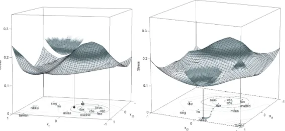
Nowadays, the acronym SMACOF stands for Scaling by Majorizing a Com-plex Function. To understand how it works consider Figure 5a. Suppose that we have dissimilarity data on 13 stock markets and that the two dimensional MDS solution is given by the points in the horizontal plane of Figure 5a and 5b. Now, suppose that the position of the ‘nikkei’ index was unknown. Then we can calculate the value of Stress as a function of the two coordinates for ‘nikkei’.
a. First majorizing function b. Final majorizing function
Figure 5: The Stress function and the majorizing function for the supporting (0,0) in Panel a., and the majorizing function at convergence in Panel b. Re-produced by permission of Vrieseborch Publishers
The surface in Figure 5a shows these values of Stress for every potential posi-tion of ‘nikkei’. To minimize Stress we must find the coordinates that yield the lowest Stress. Hence, the final point must be located in the horizontal plane under the lowest value of the surface. To find this point, we use an iterative procedure that is based on majorization. First, as an initial point for ‘nikkei’ we choose the origin in Figure 5a. Then, a so-called majorization function is chosen in such a way that, for this initial point, its value is equal to the Stress-value, and elsewhere it lies above the Stress surface. Here, the majorizing function is chosen to be quadratic and is visualized in Figure 5a as the bowl-shaped surface above the Stress function surface. Now, as the Stress surface is always below the majorization function, the value of Stress evaluated at the point correspond-ing to the minimum of the majorization function, will be lower than the initial Stress value. Hence, the initial point can be updated by calculating the mini-mum of the majorization function which is easy because the majorizing function is quadratic. Using the updated point we repeat this process until the coordi-nates remain practically constant. Figure 5b shows the subsequent coordicoordi-nates for ‘nikkei’ obtained by majorization as a line with connected dots marking the path to its final position.
8
Alternative measures for doing
Multidimen-sional Scaling
In addition to the raw Stress measure introduced in Section 3, there exist other measures for doing Stress. Here we give a short overview of some of the most popular alternatives. First, we discuss normalized raw Stress,
σ2 n(bd,X) = Pn i=2 Pi−1 j=1wij(dbij−dij(X))2 Pn i=2 Pi−1 j=1wijdb2ij , (4)
which is simply raw Stress divided by the sum of squared dissimilarities. The advantage of this measure over raw Stress is that its value is independent of the scale and the number of dissimilarities. Thus, multiplying the dissimilarities by a positive factor will not change (4) at a local minimum, whereas the coordinates will be the same up to the same factor.
The second measure is Kruskal’s Stress-1 formula
σ1(bd,X) = Ã Pn i=2 Pi−1 j=1wij(dbij−dij(X))2 Pn i=2 Pi−1 j=1wijd2ij(X) !1/2 , (5)
which is equal to the square root of raw Stress divided by the sum of squared distances. This measure is of importance because many MDS programs and publications report this value. It can be proved that at a local minimum of
σ2
n(db,X),σ1(db,X) also has a local minimum with the same configuration up to
a multiplicative constant. In addition, the square root of normalized raw Stress is equal to Stress-1 (Borg & Groenen, 1997).
A third measure is Kruskal’s Stress-2, which is similar to Stress-1 except that the denominator is based on the variance of the distances instead of the sum of squares. Stress-2 can be used to avoid the situation where all distances are almost equal.
A final measure that seems reasonably popular is called S-Stress (imple-mented in the program ALSCAL) and it measures the sum of squared er-ror between squared distances and squared dissimilarities (Takane, Young, & De Leeuw, 1977). The disadvantage of this measure is that it tends to give solutions in which large dissimilarities are overemphasized and the small dis-similarities are not well represented.
9
Pitfalls
If missing dissimilarities are present, a special problem may occur for certain patterns of missing dissimilarities. For example, if it is possible to split the objects in two or more sets such that the between-set weightswij are all zero, we are dealing with independent MDS problems, one for each set. If this situa-tion is not recognized, you may inadvertently interpret the missing between set distances. With only a few missing values, this situation is unlikely to happen.
qqqqqqqqqqqqqqqqqqqqqqqqqqqqqq q q q q q q q q q q q q q q q q q q q q q q q q q q q q q q
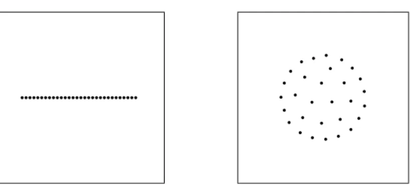
Figure 6: Solutions for constant dissimilarities withn= 30. The left plot shows the unidimensional solution and the right plot a 2D solution.
However, when dealing with many missing values, one should verify that the problem does not occur.
Another important issue is to understand what MDS will do if there is no information in the data, that is, when all dissimilarities are equal. Such a case can be seen as maximally uninformative and therefore as a null model. Solutions of empirical data should deviate from this null model. This situation was studied in great detail by Buja, Logan, Reeds, and Shepp (1994). It turned out that for constant dissimilarities, MDS will find in one dimension points equally spread on a line (see Figure 6). In two dimensions, the points lie on concentric circles (De Leeuw & Stoop, 1984) and in three dimensions (or higher), the points lie equally spaced on the surface of a sphere. Because all dissimilarities are equal, any permutation of these points yield an equally good fit.
This type of degeneracy can be easily recognized by checking the Shepard diagram. For example, if all disparities (or dissimilarities in ratio MDS) fall into a small interval considerably different from zero, we are dealing with the case of (almost) constant dissimilarities. For such a case, we advise redoing the MDS analysis with a more restrictive transformation, for example, using monotone splines, an interval transformation or even ratio MDS.
A final pitfall for MDS are local minima. A local minimum for Stress implies that small changes in the configuration always have a worse Stress than the lo-cal minimum solution. However, larger changes in the configuration may yield a lower Stress. A configuration with the overall lowest Stress value is called a global minimum. In general, MDS algorithms that minimize Stress cannot guarantee the retrieval of a global minimum. However, if the dimensionality is exactly n−1, it is known that ratio MDS only has one minimum that is consequently global. Moreover, whenp=n−1 is specified, MDS often yields a solution that fits in a dimensionality lower thann−1. If so, then this MDS solution is also a global minimum. A different case is that ofunidimensional scaling. For unidimensional scaling with a ratio transformation, it is well known that it has many local minima and can better be solved using combi-natorial methods. For low dimensionality, like p = 2 or p = 3, experiments
indicated that the number of different local minima ranges from a few to several thousands. For an overview of issues concerning local minima in ratio MDS, we refer to Groenen and Heiser (1996) and Groenen, Heiser, and Meulman (1999). When transformations are used, there are fewer local minima and the proba-bility of finding a global minimum increases. As a general strategy, we advice to use multiple random starts (say 100 random starts) and retain the solution with the lowest Stress. If most random starts end in the same candidate minimum, then there probably only exist few local minima. However, if the random starts end in many different local minima, the data exhibit a serious local minimum problem. In that case, it is advisable to increase the number of random starts and retain the best solution.
References
Borg, I., & Groenen, P. J. F. (1997). Modern multidimensional scaling: Theory and applications. New York: Springer.
Buja, A., Logan, B. F., Reeds, J. R., & Shepp, L. A. (1994). Inequalities and positive-definite functions arising from a problem in multidimensional scaling. The Annals of Statistics,22, 406–438.
De Leeuw, J. (1977). Applications of convex analysis to multidimensional scaling. In J. R. Barra, F. Brodeau, G. Romier, & B. van Cutsem (Eds.), Recent developments in statistics(pp. 133–145). Amsterdam, The Nether-lands: North-Holland.
De Leeuw, J. (1988). Convergence of the majorization method for multidimen-sional scaling. Journal of Classification,5, 163–180.
De Leeuw, J., & Heiser, W. J. (1980). Multidimensional scaling with restrictions on the configuration. In P. R. Krishnaiah (Ed.), Multivariate analysis (Vol. V, pp. 501–522). Amsterdam, The Netherlands: North-Holland. De Leeuw, J., & Stoop, I. (1984). Upper bounds of Kruskal’s Stress.
Psychome-trika, 49, 391–402.
Ekman, G. (1954). Dimensions of color vision. Journal of Psychology, 38, 467–474.
Gower, J. C., & Legendre, P. (1986). Metric and Euclidean properties of dissimilarity coefficients. Journal of Classification,3, 5–48.
Groenen, P. J. F., & Heiser, W. J. (1996). The tunneling method for global optimization in multidimensional scaling. Psychometrika,61, 529–550. Groenen, P. J. F., Heiser, W. J., & Meulman, J. J. (1999). Global optimization
in least-squares multidimensional scaling by distance smoothing. Journal of Classification,16, 225-254.
Kruskal, J. B. (1964a). Multidimensional scaling by optimizing goodness of fit to a nonmetric hypothesis. Psychometrika,29, 1–27.
Kruskal, J. B. (1964b). Nonmetric multidimensional scaling: A numerical method. Psychometrika,29, 115–129.
Meulman, J. J., Heiser, W. J., & SPSS. (1999). Spss categories 10.0. Chicago: SPSS.
Ramsay, J. O. (1988). Monotone regression splines in action.Statistical Science, 3(4), 425–461.
Spence, I., & Ogilvie, J. C. (1973). A table of expected stress values for random rankings in nonmetric multidimensional scaling. Multivariate Behavioral Research,8, 511–517.
Takane, Y., Young, F. W., & De Leeuw, J. (1977). Nonmetric individual differences multidimensional scaling: An alternating least-squares method with optimal scaling features. Psychometrika,42, 7–67.