A Method for Solving the Fleet Assignment Problem Using Detailed Parameter Calculation

A Method for Solving the Fleet Assignment Problem Using

Detailed Parameter Calculation

Marcos G. Ierides Mechanical Engineer [email protected] Nikolaos Aretakis Lecturer [email protected]

Laboratory of Thermal Turbomachines National Technical University of Athens

Iroon Polytecnhniou 9, 15780 Athens, Greece

1. ABSTRACT

The Fleet Assignment Problem (FAP) in the airline industry is related to a big number of parameters, many of which have a strong interdependence.

Throughout the last decades, a number of models for solving the fleet assignment problem have been proposed that aim to optimize the assignment upon different criteria.

In this paper, a new approach to the fleet assignment process for a fleet of civil aircraft is introduced, that aims to maximize the profit for a set of given flight legs.

The proposed approach is based on a detailed modeling of the financial figures that derive from every possible pairing of flight leg-aircraft available.

The application of the model in a case study shows the benefits of detailed modeling for solving the FAP. Particularly, engine deterioration in fuel consumption, passenger forecasting, as well as detailed airport charges estimation highly impact the solution of the problem.

2. NOMENCLATURE

Throughout the paper, the following nomenclature will be used: T: temperature

L: distance E: elevation H: hours D: duration

PD: passenger demand forecasting P: passengers

PC: passenger capacity SP: spilled passengers R: passenger revenues AE: airport expenses FE: fuel expenses CE: crew expenses NF: navigation fees

SE: maintenance routing expenses PC: passenger charges

WF: weight fees FC: consumption FP: fuel price S: crew salary RC: en route charges TC: terminal charges RU: en route unit rate TU: terminal unit rate EFC: engine flight cycle MC: maintenance cycle RWL: runway length CNL: certified noise level

EGTM: exhaust gas temperature margin Superscripts and subscripts:

f: aircraft

s: station/airport (sa for arrival station, sd for departure station)

l: flight leg/mission t: point in time

w: time window with starting point t- and end point t+ m: maintenance

p: code sharing partner

d: flight type (national, continental, global)

t: passenger type (final destination, transit, transfer) c: fare class

y: year r: crew rank h: mission phase 3. INTRODUCTION

During the year 2012, the airline industry was responsible for carrying almost 2.9 billion passengers around the globe. During the same year, the airline industry worldwide returned a profit of $6.7 billion. For the year 2013, the industry is expected to carry well above 3 billion passengers, while the returned profit is estimated to $8.4 billion.

Nevertheless, the above numbers are well below the $8.8 billion profit the industry returned in 2011, while the 1.0% net profit margin it presented in 2012 is below the 7-8% needed to recover the industry's cost of capital.

Throughout the decades of its existence, the airline industry's profit has been globally or locally affected by stochastic phenomena.

In the last years, the main reasons why the industry has failed to achieve its initial expectations can be summed to the following:

- World recession - Oil crisis

- Natural/Man-made disasters - State/Community policies

An example of the natural/man-made disasters are the eruption of Eyjafjallajökull, the 9/11 terrorist attack, while an example of community policies is the EU resolution regarding Malèv airline loans from the Hungarian government, that brought the company to bankruptcy in 2012.

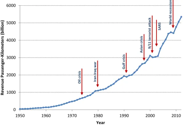
In Figure 1, one can see how the industry has been affected by various worldwide phenomena in the last decades.

Figure 1: World aviation growth from 1950 to 2012 (source: ICAO)

Since the above phenomena have a great effect on the flow of passengers, and as a result, on the profit of the industry, the airline companies have been striving to maximize their profit through optimizing their operational functions.

One of the functions that has a high impact on the operating costs (and thus the profit) is the fleet assignment. For this reason, the airline companies have been striving to optimize the way they solve the Fleet Assignment Problem. Various models have been proposed since the first attempts of optimizing the process in the 1950's.

In this paper, an attempt is made to combine the strengths of the most prevalent models, as well to overcome their weaknesses, in order to propose a new, improved model for solving the Fleet Assignment Problem.

The proposed model also includes innovative characteristics which include detailed fuel consumption estimation considering engine deterioration, passenger demand forecasting, detailed airport expenses calculation, and others.

The research subject studied in the present paper is the Fleet Assignment Problem. Given a set of flight legs that have to be performed from a given station during a specific period of time, and given the available aircraft, we attempt to find the best possible assignment of aircraft to flight legs that will generate the maximum profit.

More specifically, in this paper, a proposal for a new approach for solving the FAP is made, aiming to maximize the profit through increasing the revenues for a given set of flight legs, and decreasing the operational expenses. 0 1000 2000 3000 4000 5000 6000 1950 1960 1970 1980 1990 2000 2010 R e ve n u e Pas sen ge r-K ilo m e te rs (b ill io n ) Year O il cr is is G ul f cr is is A si an cr is is 9/ 11 t er rori st a tt ack SA R S Worl d r e ce ss ion Ir an -Ir aq war

In order to achieve the optimized fleet assignment, a more precise modeling of the financial figures for each aircraft-flight leg pairing is presented. Subsequently, we propose a set of algorithms that point the combination of aircraft-flight legs that generate the highest profit, or in case of loss, the lowest loss.

Throughout the development of the proposed model, works of previous research teams was studied, and some of the characteristics were based on previous research. Namely, the works of (Abara 1989) set a strong influence on the models dealing with the FAP, since it was among the first attempting to optimize the process. Nevertheless, the model has some limitations due to the choice of connection arcs as decision variables. Since the introduction of the model by Abara, a number of variations have been introduced.

Advancements in the field brought the introduction of integrated models˙ (Barnhart, Kniker and Lohatepanont 2002) introduce the effects of spill and recapture, as well as integration of a more detailed demand and fare modeling for higher precision on revenue estimation.

Other models introduce integration with other operational areas closely related to fleet assignment˙ (Clarke, et al. 1996) consider crew and maintenance planning in fleet assignment. (Lapp and Cohn 2012) include maintenance routing in order to optimize the fleet assignment, while (Walid and Felix 2000) introduce fleet assignment considering a more dynamic approach to maintenance scheduling.

(Rexing, et al. 2000) and (Belanger, et al. 2006) integrate fleet assignment with schedule planning by introducing flexible departure times.

Although the above works introduce several innovations in the FAP optimization, we believe there are several shortcomings, which the model presented aims to overcome:

‐ Integration of Accurate Financial Modeling

The above models heavily rely on optimizing the fleet assignment process through optimizing the mathematical formulation of the fleet assignment algorithm thus neglecting the modeling of revenues and expenses, or relying on other models for that purpose

The presented model introduces an integrated model that performs accurate financial figures modeling thus aiming to optimize the process by targeting basic elements of the problem.

‐ Aircraft Level Modeling

Fleet assignment models distinguish aircraft on a fleet type level. In this way, several generalizations and assumptions are made, for the state of each aircraft.

The presented model introduces aircraft level modeling by considering engine deterioration for every unique aircraft by associating engine flight cycle with engine health index.

‐ Passenger Demand Forecasting

A forecasting algorithm for estimating passenger demand for each unique flight leg using data from previous years is integrated in the model presented here. The algorithm can be adjusted for stochastic or periodic phenomena that affect passenger traffic locally or globally (e.g. natural disasters, Olympic Games)

The paper outline is as follows:

In section 4, the parameters that are taken under consideration for solving the FAP through the introduced model are presented.

In section 5 the developed model is presented˙ its characteristics, the steps it follows to solve the FAP, as well as the mathematical formulation of the parameters.

In section 6 the implementation of the model is presented˙ the results of a case study as well as the sensitivity analysis conducted.

Section 7, includes a summary, along with conclusions and suggestions for future steps for the development of the model.

4. PARAMETERS CONSIDERED

For the development of the current model, the parameters that rule the flight leg-aircraft pairing and its financial figures were narrowed down to the ones that have the highest impact on the final decision.

The parameters could be further split into restrictions, and criteria.

Restrictions are the parameters that need to be fulfilled in order for the aircraft to be able to perform the given flight leg, while criteria are the parameters which have an impact on the financial figures (revenues and expenses) that derive from an aircraft-flight leg pairing.

They are the following: 4.1. Restrictions

4.1.1. Airport Restrictions

According to the departure or arrival airport of a flight leg, there are various restrictions that need to be met for the departing or arriving aircraft.

‐ Runway Length

The runway length needed for landing or take-off for a specific aircraft varies according to its weight, aerodynamic characteristics, ambient temperature, and the altitude. For the aircraft to be permitted a landing or take-off, the airport runway needs to be long enough for the aircraft to be able to perform a landing or take-off.

‐ Noise Emissions

As several airports are situated close to inhabited areas, they might impose noise level restrictions, for several time periods during the day.

‐ Aircraft Ownership

Particular airports might request that the aircraft using their premises are owned by the airline companies operating them (and not under rent or lease)

4.1.2. Aircraft Restrictions

These are the restrictions that need to be met in order for the aircraft to be operational and able to perform a flight. The restrictions are not met if the aircraft is not available at the specified time at the station under consideration (under maintenance etc.)

4.1.3. Code Sharing Partners Restrictions

As company alliances are growing bigger in number and diversity, the need for regulations that assures the quality of the services provided by the members of a given alliance has been raising. These restrictions might require that the aircraft performing a flight under an alliance name will fulfill characteristics such inflight entertainment system, first class section, etc.

4.2. Criteria

4.2.1. Passenger Revenues

For a commercial flight, the revenues derive from the passengers on the flight. 4.2.2. Airport Charges

These are expenses imposed by the departing and arriving airport for each flight leg. 4.2.3. Fuel Expenses

A big part of the expenses for each flight is the cost fuel which are subject on the consumed fuel during the mission.

4.2.4. Crew Expenses

These expenses include crew salaries for the duration of each flight. 4.2.5. Air Navigation Fees

Air navigation fees are implied by the states of which the airspace or ground is used. They are described in detail in paragraph 5.2.8.

4.2.6. Maintenance

Maintenance is among the highest expenses in an operational airline company. For the modeling of maintenance expenses the following two aspects are considered:

‐ Maintenance Routing

This aspect deals with routing the aircraft that need to undergo maintenance to maintenance stations. ‐ Exploitation of Remaining Flight Hours

Aircraft need to undergo maintenance either because they have completed a specific number of flight hours, or because a certain time period has passed since the last maintenance, whichever comes first. This aspects deals with exploiting the remaining flight hours before the next planned maintenance.

5. THE PROPOSED MODEL

The fleet assignment is a repeating process that happens throughout the entire day, in an operational airline company. In order for the presented model to be applicable throughout the day, it was deemed necessary to split the day in discrete periods of time (or "time windows"). Then, and since the list of available aircraft for the specific time window, as well as the flight legs that need to be performed are known, the flight and financial parameters that result from each possible pairing aircraft-flight leg are computed. Subsequently, the feasible combination that generates the highest profit (or minimum loss) is proposed.

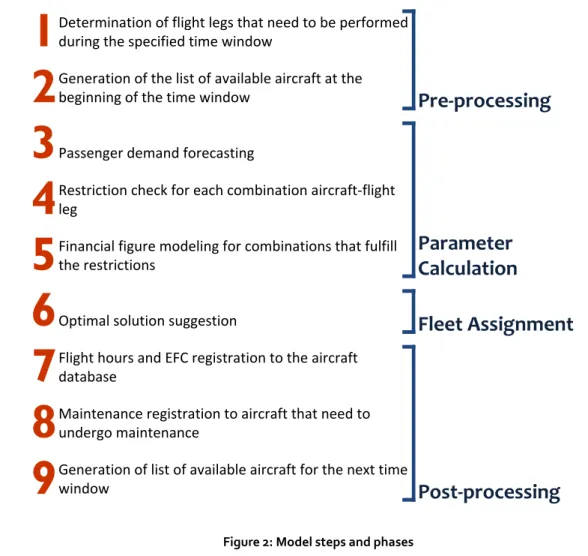
The procedure described above is repeated for each consecutive time window as to optimize a day period. The steps of this procedure are shown in Figure 2.

Figure 2: Model steps and phases Determination of flight legs that need to be performed during the specified time window

Generation of the list of available aircraft at the beginning of the time window

1

2

Passenger demand forecasting

3

Restriction check for each combination aircraft-flight leg

Financial figure modeling for combinations that fulfill the restrictions

Flight hours and EFC registration to the aircraft database

Maintenance registration to aircraft that need to undergo maintenance

Generation of list of available aircraft for the next time window

4

5

7

8

9

Pre-processing

Parameter

Calculation

6

Post-processing

Fleet Assignment

The steps can be grouped in four different phases.

In the pre-processing phase, the list of available aircraft, as well as the flight legs that need to be performed in the specific time-window is being generated.

In the parameter calculation phase, the passenger demand for each flight leg is estimated using forecasting techniques with data from previous years. Then, a constrain check is performed, in order to examine which pairing aircraft-flight legs are feasible. This is done as to reduce the computational time by computing the financial parameters for only the flight leg-aircraft pairs that fulfill the restrictions. In the end of this phase, the modeling of each parameter takes place.

In the fleet assignment phase, the possible combinations of flight leg-aircraft pairs are checked, and the one that generates the highest profit (or minimum loss) is proposed.

Lastly, in order to be able to repeat the above steps for the next time window, the data have to be post-processed. This phase includes registering flight hours to the aircraft that have performed a flight, registering maintenance to the aircraft that need to undergo maintenance, and generating the list of available aircraft for the next time window.

In the following paragraphs, a more detailed description of the steps and the modeling of the parameters is presented. Additionally, examples are given, for better understanding by the reader.

5.1. Pre-processing 5.1.1. Flight Legs

Having designated the station and timing, the first step is to specify the flight legs that need to be performed out of the flight schedule of the airline company.

The developed algorithm reads through the flight schedule of the airline under consideration. For every flight of which the departing station matches the station under consideration and the departure time is included in the time window, the flight data is copied to a list (matrix) which includes all the flights that need to be performed in the specific time window.

5.1.2. Aircraft

Similar to the above, the list of available aircraft is generated by identifying the aircraft that are present at the station under consideration in the beginning of the time window.

5.2. Parameter Calculation 5.2.1. Airport Restrictions ‐ Runway Length

For the model, the runway requirements for each aircraft, at sea level, for standard day temperature is considered. The data are then deduced in order to calculate the runway requirements for the ambient characteristics and altitude of the given airport.

In order to avoid extra calculations, we assume that each aircraft landing at a station will have to depart from it at one point in the near future so that the ambient temperature will not change significantly. Since the take-off length requirements are higher than landing requirements for a given aircraft, only take-off runway requirements need to be fulfilled, for a given aircraft.

For runway length adjustment, the approach of (Embraer n.d.) is used, while for aircraft data, the BADA database (Base of Aircraft Data) is used.

The approach assumes an increase of 7% at the necessary take-off length for every 1000 feet above sea level, and a 5% increase for every Fahrenheit degree above standard day temperature (59˚F).

The above is modeled as follows:

𝐿_𝑓 = 0.005 ∙ (𝑇_𝑠𝑎 − 𝑇_𝑠𝑎𝑠_{𝑎 ) ∙ 𝐿} 𝑓𝑠𝑎 𝑎 _{+ 𝐿}

𝑓𝑠𝑎

Where,

𝑇_𝑠𝑎𝑠_{𝑎 = 𝑇}𝑠_{− (}3.566 ∙ 𝐸𝑠

1000 ) (2) 𝐿_𝑓𝑠𝑎_{𝑎 = (}0.07 ∙ 𝐸𝑠

1000 ) + 𝐿𝑓𝑠𝑙 (3)

Lf: adjusted take-off distance for aircraft f

𝑇𝑠𝑎: ambient temperature at the arrival station (in Fahrenheit)

𝑇_𝑠𝑎𝑠_{𝑎: adjusted standard temperature at the arrival station altitude}

Ts: standard day temperature

𝐿_𝑓𝑠𝑎_{𝑎: adjusted runway length for aircraft f, at the arrival station altitude}

𝐿_𝑓𝑠𝑙_{: necessary runway length for aircraft f at sea level}

‐ Noise Emissions

In order to check whether each aircraft complies with the restrictions, the approach noise level (in EPNdB) for each aircraft has been taken into consideration. For aircraft noise emission, the NoisedB database has been used (ICAO 2012). The restrictions that need to be met is formulated as follows:

𝑁𝐿_𝑓𝑎𝑝𝑝 ≤ 𝐶𝑁𝐿𝑠𝑤 (4)

Where,

𝑁𝐿_𝑓𝑎𝑝𝑝: emmited noise level during approach phase for aircraft f

CNLsw: noise emission allowance for station s during time window w

‐ Aircraft Ownership

In order for the aircraft to comply with ownership restrictions (if any) the following should be met: 𝐴𝑂𝑓 ≥ 𝐴𝑂𝑅𝑠 (5)

Where,

AOf: binary variable that is: 1 if aircraft f is owned by the airline company under consideration, 0 otherwise AORs: binary variable that is: 1 if station s sets ownership restrictions, 0 otherwise

5.2.2. Aircraft Restrictions

In order for the aircraft to be operational, all the required check types and maintenance needs to have been performed. The above is modeled as follows:

𝐻𝑚𝑖 ≥ 𝐷𝑙 (6)

Where,

𝐻_𝑚𝑖: remaining hours until next type i maintenance (in hr)

Dl: duration of flight leg l (in hr)

These restrictions are modeled as follows:

𝑆𝑓𝑖 ≥ 𝐼𝑙𝑝∙ 𝑅𝑝𝑖 (7)

Where,

Sfi: binary variable that is: 1 if aircraft f complies with specification i, and 0 otherwise Ilp: binary variable that is: 1 if flight leg l has a shared code with partner p, and 0 otherwise

Rpi: binary variable that is: 1 if partner p sets restrictions regarding specification i, and 0 otherwise

5.2.4. Passenger Revenues

In order to model the passenger revenues, an estimated demand should be calculated. For this purpose, a forecasting algorithm has been developed, which estimates the demand for each particular flight, using previous years’ data. For revenue calculation three fare classes are considered. Additionally, spilled and recaptured passengers are taken into consideration (Barnhart, Kniker and Lohatepanont 2002).

The mathematical formulation of the algorithm:

𝑃𝐷𝑡𝑑𝑐𝑙 = ((∑ 𝛥𝑃𝐷𝑦𝑡𝑑𝑐𝑙∙ 𝐶𝑦 𝑛𝑦 𝑦=1 ) + 1) ∙ 𝑃𝐷_𝑦+_{𝑡𝑑𝑐𝑙}, ∀𝑡 ∈ 𝑛_𝑡𝑙, 𝑑 ∈ 𝑛_𝑑𝑙, 𝑐 ∈ 𝑛_𝑐𝑙 (8) Subject to, ∑ 𝐶𝑦 𝑛𝑦 𝑦=1 = 1 (9) Where,

PDtdcl: forecasted passenger demand for passenger type t, flight type d, class c, for flight leg l

ΔPDytdcl: the difference between passenger demand for passenger type p, flight type d, type t, class c, for

flight leg l, between two consecutive years

Cy: weight coefficient for year y

𝑃𝐷_𝑦+_{𝑡𝑑𝑐𝑙}:demand of passengers type t, flight type d, class c, for flight leg l, for the last year for which data is

available

For better understanding of the forecasting algorithm, the following example is illustrated:

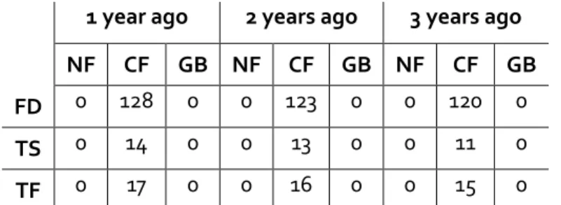
Consider the flight leg A-B, which is a part of itineraries A-B-C, and A-B-D. Considering that flight leg B-C is carried by the same aircraft as A-B (through flights), this implies that on board flight A-B, we will have passengers of which the final destination is B (FD), transit passengers of which the final destination is C (TS), and transfer passengers of which the final destination is D (TF). Furthermore, consider that flight A-B is a continental flight (CF). The example is illustrated in Table 1.

1 year ago 2 years ago 3 years ago NF CF GB NF CF GB NF CF GB FD 0 128 0 0 123 0 0 120 0 TS 0 14 0 0 13 0 0 11 0 TF 0 17 0 0 16 0 0 15 0 Table 1: Previous years’ economy class passenger demand for flight leg A-B

Applying equation (8) for economy class passenger demand forecasting, and considering the weight coefficient for the last year as 0.6, we have:

PD[FD][C][E][AB] = [(((123-120)/120)x0.4+((128-123)/123)x0.6)+1]x128 ⇒ PD[FD][C][E][AB] = 132.402

The final value is rounded to the nearest integer.

We repeat the process for all passenger classes (first class, business) and types (transfer -TF, transit -TS). Having estimated the passenger demand, the next step is to estimate the number of passengers on the aircraft in accordance to its capacity.

In case that passenger demand is higher than the available capacity, a number of passengers needs to be rejected (spilled passengers). In that case, the transit passengers are the ones rejected first. If all transit passengers are rejected, and the demand is still higher than the capacity, transfer passengers are rejected.

As one can see, the final destination passengers are the ones most favorable by the algorithm, while transit passengers are the ones least favorable. This happens because final destination passenger’s fare per mile is higher than transfer fares, which are higher than transit fares per mile.

The mathematical formulation:

𝑃𝑐𝑙𝑓 = ∑ ∑ min⁡{𝑃𝐷𝑡𝑑𝑐𝑙 𝑛𝑑𝑙 𝑑=1 𝑛𝑡𝑙 𝑡=1 , ⁡𝑃𝐶𝑐𝑓 − ∑ 𝑃𝑐𝑙_𝑖} 𝑡−1 𝑖=1 , ∀𝑐 ∈ 𝑛𝑐𝑓 (10) Where,

Pclf: class c passengers onboard aircraft f, if it performs flight leg l

PDtdcl: passenger demand of passengers type t, flight type d, class c, for flight leg l PCcf: passenger capacity for class c, on aircraft f

ntl: total passenger types on flight leg l ndl: total flight types on flight l

ncf: total passenger classes on aircraft f

Since the model includes revenues from recaptured passengers, an estimation of spilled passengers is needed: 𝑆𝑃_𝑐𝑙𝑓 = ∑ ∑ |min⁡{ 𝑛𝑑𝑙 𝑑=1 𝑛𝑡𝑙 𝑡=1 (𝑃𝐶_𝑐𝑓− ∑ 𝑃𝐷_𝑐𝑙𝑖 𝑡−1 𝑖=1 ) , 0}|, ∀𝑐 ∈ 𝑛_𝑐𝑓 (11)

Finally, for calculating passenger revenues, from both actual and recaptured passengers, we multiply each passenger class with the according fare:

𝑅𝑙𝑓 = ∑ 𝑅𝑐𝑙𝑓 𝑛𝑐𝑓

𝑐=1

Where,

𝑅𝑐𝑙𝑓= 𝐹𝑐𝑙∙ 𝑃𝑐𝑙𝑓+ 𝑆𝑃𝑐𝑙𝑓∙ 𝐹𝑐𝑙∙ 𝑅𝑅𝑐𝑙, ∀𝑐 ∈ 𝑛𝑐𝑓 (13)

Rclf: revenues from class c passengers, if aircraft f performs flight leg l Fcl: fare of class c, for flight leg l

Pclf: passengers of class c onboard aircraft f, if it performs flight leg l RRcl: recapture rate for class c passengers, for flight leg l

Since the fares undergo large fluctuations according to the time of booking, we suggest that the fare value for each fare class be taken as the average value of the total tickets sold for the same flight during the previous years, for each class.

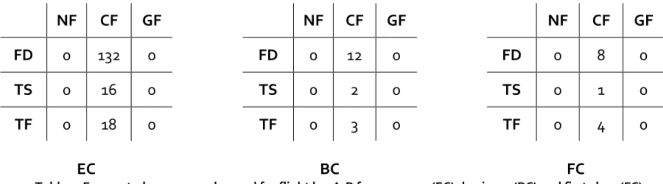
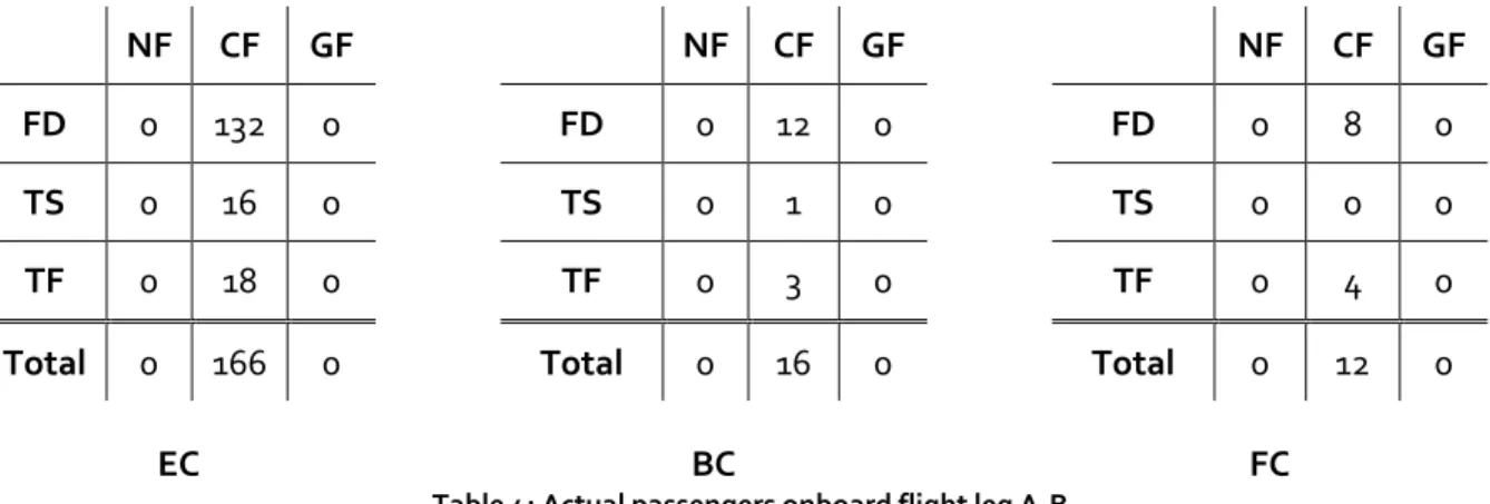
Continuing the example given previously, consider the passenger demand forecast for itinerary A-B that is illustrated in Table 2. NF CF GF NF CF GF NF CF GF FD 0 132 0 FD 0 12 0 FD 0 8 0 TS 0 16 0 TS 0 2 0 TS 0 1 0 TF 0 18 0 TF 0 3 0 TF 0 4 0 EC BC FC

Table 2: Forecasted passenger demand for flight leg A-B for economy (EC), business (BC) and first class (FC)

The three individual tables refer to the passenger demand for economy class (EC), business class (BC) and first class (FC).

Consider that the aircraft capacity for each class is the one illustrated in Table 3.

EC BC FC

168 16 12

Table 3: Aircraft passenger capacity for each fare class

Using equation (10) we calculate the total number of actual passengers, for each passenger class. For economy class:

P [C][E][AB]=min{168,132}+min{16,(168-132)}+min{18,(168-(132+16))} ⇒ P [C][E][AB]=166

The same process is repeated for each passenger class, and the resulting number of actual passengers per type is illustrated in Table 4.

NF CF GF NF CF GF NF CF GF

FD 0 132 0 FD 0 12 0 FD 0 8 0

TS 0 16 0 TS 0 1 0 TS 0 0 0

TF 0 18 0 TF 0 3 0 TF 0 4 0

Total 0 166 0 Total 0 16 0 Total 0 12 0

EC BC FC

Table 4: Actual passengers onboard flight leg A-B

Using equation (11), we estimate the spilled passengers. The results of the total actual and spilled passengers are illustrated in Table 5.

EC BC FC P 166 16 12

SP 0 1 1

Table 5: Actual and spilled passengers for flight leg A-B

5.2.5. Airport Charges

Airport charges are depending on aircraft weight, flight type (national, continental, global), as well as passenger number.

For more precise airport charges modeling, aircraft MTOW is taken into consideration. As for passengers, they are further categorized according to destination (national, continental, global) and type (final destination, transit, transfer).

Specifically, the estimation of airport expenses include aircraft charges according to MTOW, and passenger charges according to their destination and flight type.

The above is modeled as follows:

𝐴𝐸𝑙𝑓 = 𝑃𝐶𝑙𝑓+ 𝐴𝐶𝑙𝑓 (14) Where, 𝑃𝐶_𝑙𝑓 = ∑ ∑ 𝐴𝐹_𝑡𝑑𝑠∙ 𝑛𝑑𝑙 𝑑=1 𝑃_{𝑡𝑑𝑙𝑓} 𝑛𝑡𝑙 𝑡=1 + 𝑃_𝑙𝑓∙ 𝑂𝐹_𝑠 (15) 𝐴𝐶_𝑙𝑓 = 𝑀𝑇𝑂𝑊_𝑓∙ (𝑊𝐹_𝑠𝑑+ 𝑊𝐹_𝑠𝑎) (16) Subject to, 𝑃_{𝑡𝑑𝑙𝑓} = ∑ 𝑃_{𝑐𝑡𝑑𝑙𝑓} 𝑛𝑐𝑓 𝑐=1 (17)

𝑃_𝑙𝑓 = ∑ 𝑃_𝑐𝑙𝑓

𝑛𝑐𝑓

𝑐

(18)

AElf: airport charges if flight leg l is performed by aircraft f

PClf: airport charges concerning passengers if flight leg l is performed by aircraft f AClf: airport charges concerning aircraft if flight leg l is performed by aircraft f AFtds: fee charged by airport s for passenger type s, on flight type d

Ptdlf: passengers of type t, on flight type d on board flight leg l, if it is performed by aircraft f OFs: other fees per passenger at airport s

MTOWf: Maximum Take Off Weight of aircraft f (in tn)

𝑊𝐹𝑠𝑑: fees (per tn) at the departing station s

𝑊𝐹_𝑠𝑎: fees (per tn) at the arriving station s 5.2.6. Fuel Expenses

For estimating the fuel consumption, a detailed five-stage mission analysis model is used (Kelaidis, et al. 2009). For precise modeling, the following is taken into consideration:

- Aircraft type & engines - Aircraft weight

- Engine deterioration - Wind velocity

- Fuel price (at the departing airport)

Fuel expenses estimation algorithm uses the mission analysis model to estimate fuel consumption according to aircraft weight. Subsequently, the effects of engine deterioration, and wind velocity are taken into consideration, and the fuel consumption is adjusted using the proper coefficients.

The mathematical formulation:

𝐹𝐸𝑙𝑓 = 𝐹𝐶𝑙𝑓 ∙ 𝐹𝑃𝑠 (19) Where, 𝐹𝐶_𝑙𝑓 = 𝐶_𝑟𝑙∙ (∑ 𝐹𝐶_𝑙𝑓ℎ 𝑛ℎ ℎ=1 + 𝐹𝐶_𝑙𝑓𝑤+ 𝐹𝐶_𝑙𝑓𝑒) (20) 𝐹𝐶𝑙𝑓𝑤 = 𝑊𝑉𝑙∙ 𝐶𝑤∙ ∑ 𝐹𝐶𝑙𝑓ℎ 𝑛ℎ ℎ=1 (21) 𝐹𝐶_𝑙𝑓𝑒 = (𝑀𝐸𝐺𝑇𝑀_𝑓− 𝐸𝐺𝑇𝑀_𝑓) ∙ 𝐶_{𝐸𝐺𝑇𝑀𝑓}∙ ∑ 𝐹𝐶_𝑙𝑓ℎ 𝑛ℎ ℎ=1 (22)

FElf: fuel expenses, if flight leg l is performed by aircraft f

FClf: fuel consumption if flight leg l is performed by aircraft f (in kg) FPs: fuel price at airport s (in €/kg)

FClfh: fuel consumption for mission phase h of flight leg l if it is performed by aircraft f (for non-deteriorated

engines) (in kg)

Crl: reserve fuel coefficient for flight leg l

FClfw: fuel consumption alteration due to wind velocity w on flight l FClfe: fuel consumption alteration due to engine deterioration EGTMf: EGT margin for engines on aircraft f (in ˚C)

MEGTMf: maximum EGT margin for engines on aircraft f (σε ˚C)

CEGTMf: EGT margin coefficient on fuel consumption WVl: average headwind velocity (in m/s) on flight l Cw: wind coefficient on fuel consumption

Aircraft weight is includes empty aircraft weight, passenger, luggage, and fuel weight. It is estimated using the following:

𝑇𝑂𝑊_𝑙𝑓 = 𝑃_𝑙𝑓∙ 102 + 𝐸𝑇𝑂𝑊_𝑓+ 𝐹𝐶_𝑙𝑓 (23) Where,

TOWlf: Take Off Weight of aircraft f, performing flight leg l (in tn) ETOWf: Empty Take Off Weight

Average passenger weight is assumed at 77kg, an additional weight of 20kg for check-in luggage, and 5kg of carry-on luggage, thus reaching 102kg per passenger. For more information regarding passenger and luggage weight, the reader can refer to the works of (Walpole, et al. 2012) and (Civil Aviation Safety Authority 1990).

For better approximation of the consumed fuel, an iterative technique is being used. For the first iteration, the aircraft weight is assumed for maximum fuel capacity, thus calculating the consumed fuel for the specific aircraft weight. Subsequently, for the estimated consumed fuel weight, an iteration is performed, calculating a more realistic fuel consumption.

The wind coefficient is taken as (2.83/23)% as described in (Yaworski, Dinges and Iovinelli 2011).

The association of fuel consumption and engine deterioration is achieved using EGTM coefficient (Exhaust Gas Temperature Margin), and is modeled as follows:

𝐸𝐺𝑇𝑀𝑓 = 𝑀𝐸𝐺𝑇𝑀𝑓− (𝛥𝐸𝐺𝑇𝑢𝑓+ 𝛥𝐸𝐺𝑇𝑎𝑓) (24) Where, 𝛥𝐸𝐺𝑇_𝑢𝑓 = 𝐸𝐹𝐶_𝑓∙ (12 1000⁄ ),⁡⁡⁡⁡⁡⁡⁡⁡⁡⁡⁡⁡⁡⁡⁡⁡⁡⁡⁡⁡⁡⁡⁡⁡⁡⁡⁡⁡⁡⁡⁡⁡⁡⁡⁡⁡⁡⁡⁡⁡⁡⁡⁡⁡⁡⁡𝑓𝑜𝑟⁡0 ≤ 𝐸𝐹𝐶_𝑓 < 1000 (25) ⁡⁡⁡⁡⁡⁡⁡⁡⁡⁡⁡⁡⁡⁡⁡⁡⁡⁡⁡⁡⁡⁡⁡⁡⁡⁡(𝐸𝐹𝐶_𝑓− 1000) ∙ (6/1000) + 12,⁡⁡⁡⁡⁡⁡⁡⁡⁡⁡⁡⁡⁡⁡⁡⁡⁡⁡⁡⁡𝑓𝑜𝑟⁡1000 ≤ 𝐸𝐹𝐶_𝑓 < 2000 ⁡⁡⁡⁡⁡⁡⁡⁡⁡⁡⁡⁡⁡⁡⁡⁡⁡⁡⁡⁡⁡⁡⁡⁡⁡⁡(𝐸𝐹𝐶𝑓− 2000) ∙ (4/1000) + 12 + 6,⁡⁡⁡⁡⁡⁡⁡⁡⁡⁡⁡⁡𝑓𝑜𝑟⁡2000 ≤ 𝐸𝐹𝐶𝑓 < 5000 𝛥𝐸𝐺𝑇𝑎𝑓= 𝑀𝐶𝑓∙ 𝐶𝑟𝑒𝑚∙ 𝑀𝐸𝐺𝑇𝑀𝑓 (26)

ΔEGTuf: EGT alteration due to usage for engines of aircraft f ΔEGTaf: EGT alteration due to aging for engines aircraft f EFCf: engine cycles since last engine maintenance of aircraft f MCf: total maintenance cycles of aircraft f

As one can see from equations (29-31), for EGT alteration two deteriorating parameters are considered: (i) due to usage and (ii) due to engine aging.

For engine usage, we consider 0.012˚C EGTM alteration per flight cycle for the first 1000 cycles, 0.006˚C for the next 1000 cycles, and 0.004˚C for the rest 3000 cycles. We also consider 30% residual deterioration after each engine maintenance cycle (Aircraft Owner's & Operator's Guide 2006).

In order to calculate the flight leg distance, we use the great-circle distance method, considering the earth as a perfect sphere. The flight leg distance is considered as the straight line on the surface of the earth connecting the departure and arrival station, and it is calculated as follows:

𝐿𝑙 = 𝑟 ∙ 𝛥𝜎̂ (27)

Where,

𝛥𝜎̂ = cos−1_{(sin 𝜑}

𝑠𝑑∙ sin 𝜑𝑠𝑎+ cos 𝜑𝑠𝑑∙ cos 𝜑𝑠𝑎∙ cos 𝛥𝜆) (28)

𝛥𝜆 = |𝜆_𝑠𝑑− 𝜆_𝑠𝑎| (29)

Ll: leg distance (in m)

r: average earth radius (in m)

𝛥𝜎̂: central angle between departure and arrival station (in rad) 𝜑𝑠𝑑: geographical latitude of departure station

𝜑_𝑠𝑎: geographical latitude of arrival station 𝜆𝑠𝑑: geographical longitude of departure station

𝜆_𝑠𝑎: geographical longitude of arrival station

Although the real flight plans for a flight leg do not consist of a straight line connecting two points on the earth, the advantages of the method (simplicity, smaller computational time) are significantly more than the error it introduces. Moreover, deducing all flight distances to straight lines on the surface of the earth minimizes the error.

5.2.7. Crew Expenses

For estimating the crew expenses for each particular flight, the following are taken into consideration: - Aircraft crew demand (crew needed in order for the aircraft to be operational)

- Trip duration - Crew hourly salary

Crew expenses are estimated using crew salaries per flight minute as follows:

𝐶𝐸_𝑙𝑓 = ∑ 𝐶_𝑟𝑙𝑓∙

𝑛𝑟𝑓

𝑟

(𝑆_𝑟/60) ∙ (𝐷_𝑙+ 90 + 60) (30) Where,

CElf: crew expenses if flight leg l is performed by aircraft f

Crlf: total number of rank r crew members needed in order for aircraft f to be able to perform flight leg l Sr: hourly salary (per flight minute) of rank r crew member

Since crew shift starts 90 minutes before and ends 60 minutes after the flight, numbers 90 and 60 are added in the estimation algorithm.

5.2.8. Air Navigation Fees

These expenses consist of the following (Castelli and Ranieri n.d.): ‐ En Route Charges

In order for a flight leg to be performed, an aircraft needs to cross the airspace of at least two states. En route charges are payable to the states of which the airspace is crossed during a journey. It is subject to the following:

- Aircraft weight - Distance

‐ Terminal Charges

Payable to the state authorities of which the airport belongs to, they depend or aircraft weight. Navigation fees are modeled as followed:

𝑁𝐹_𝑙𝑓 = 𝑅𝐶_𝑙𝑓+ 𝑇𝐶_𝑙𝑓 (31) Where, 𝑅𝐶𝑙𝑓 = 𝐿_𝑙∙ 1000 − 𝑛_𝑡𝑜𝑙∙ 20 100 ∙ √ 𝑀𝑇𝑂𝑊_𝑓 50 ∙ 𝑅𝑈𝑙 (32) 𝑇𝐶_𝑙𝑓 = (𝑀𝑇𝑂𝑊𝑓 50 ) 0.7 ∙ 𝑇𝑈_𝑙 (33)

NFlf: navigation fees if flight leg l is performed by aircraft f RClf: en route charges if flight leg l is performed by aircraft f TClf: terminal charges if flight leg l is performed by aircraft f RUl: en route unit rate (in €/km∙tn)

TUl: terminal unit rate (in €/tn)

ntol: total number of take-offs performed during flight leg l

5.2.9. Maintenance ‐ Maintenance Routing

For the development of the model, aircraft maintenance is assumed to take place during the night (after23:59 and before 06:00), at designated airports were the company under consideration operates maintenance stations.

Therefore, it is favorable that the aircraft that need to undergo maintenance by the end of the night finish their day at an airport which includes a maintenance station.

In case that does not happen, the “swapcost” for that aircraft is estimated (using the above algorithms), and added to the flight expenses for the particular combination, before the optimization occurs. Swapcost consists of the total expenses needed for the aircraft to fly (empty) to the central maintenance station (fuel, navigation fees, etc.) plus the expenses for a back-up aircraft of the same fleet type to substitute the previous aircraft (fly from the central station to the departing station of the previous aircraft) in order to preserve the continuity of the network.

In order to specify which aircraft needs to undergo maintenance at the end of the day, we first calculate the maximum flight hours per day, per aircraft for the company under consideration. The aircraft starting their day with less than twice the maximum flight hours per day, per A/C are assumed that they need to undergo maintenance at the end of the day.

Maintenance routing expenses are modeled as followed:

𝑆𝐸_𝑙𝑓 = 𝑀_𝑚𝑖𝑓∙ 𝑆_𝑠𝑎∙ 𝐼_𝑤 ∙ (𝑆𝐶_𝑙𝑚𝑓+ 𝑆𝐶_{𝑙𝑚𝑓𝑟}) (34) Where,

𝑆𝐶𝑙𝑚𝑓 = 𝛢𝛦𝑙𝑚𝑓+ 𝐶𝛦𝑙𝑚𝑓+ 𝐹𝛦𝑙𝑚𝑓+ 𝑁𝛦𝑙𝑚𝑓 (35)

𝑆𝐶_{𝑙𝑚𝑓𝑟} = 𝛢𝛦_{𝑙𝑚𝑓𝑟}+ 𝐶𝛦_{𝑙𝑚𝑓𝑟}+ 𝐹𝛦_{𝑙𝑚𝑓𝑟} + 𝑁𝛦_{𝑙𝑚𝑓𝑟} (36)

SElf: maintenance routing expenses if aircraft f performs flight leg l

𝑀𝑚𝑖𝑓: binary variable that is: 1 if aircraft f needs to undergo type i maintenance at the end of the day, 0

otherwise

𝑆_𝑠𝑎: binary variable that is: 0 if the airline under consideration has a maintenance station at the arrival airport, 1 otherwise

Iw: binary variable that is: 1 if flight leg l is the last flight of the day for the specific aircraft, 0 otherwise

𝑆𝐶𝑙𝑚𝑓: total cost for the aircraft f (needing to undergo maintenance) to perform a flight to the central

maintenance station

𝑆𝐶_{𝑙𝑚𝑓𝑟}: total cost for the back-up aircraft to perform a flight from the central maintenance station to the arrival station of flight leg l

‐ Exploitation of Remaining Flight Hours

Considering that assigning longer flight legs to aircraft that need to undergo maintenance is wanted, the pairings that consist of long flight legs, and aircraft that have a planned maintenance soon need to be prioritized. In order to achieve that, the longest flights in each time window are identified, as well as the aircraft that need to undergo maintenance at the end of the day. Then, a 5% bonus (on the estimated revenues of the combination) is given if the flight leg duration is from 75% up to 100% of the duration of the longest flight leg in the time window (which would include the longest flight), and 2% if it is from 50% up to 74.99% of the longest duration. This “artificial” bonus is given only to prioritize the specific pairings, and does not represent the actual revenues.

The above is modeled as follows:

𝐵𝐶𝑙𝑓⁡ = 0.05,⁡⁡⁡⁡⁡⁡⁡⁡⁡⁡⁡⁡⁡⁡⁡⁡𝑓𝑜𝑟⁡⁡ 𝐷𝑚𝑎𝑥𝑙⁄ ≥ 0.75 _𝐷𝑙 (37) ⁡⁡⁡⁡⁡⁡⁡⁡⁡⁡⁡= 0.025,⁡⁡⁡⁡⁡⁡⁡⁡⁡⁡⁡⁡⁡𝑓𝑜𝑟⁡⁡0.5 ≤ 𝐷𝑚𝑎𝑥𝑙 𝐷𝑙 ⁄ < 0.75 = 0,⁡⁡⁡⁡⁡⁡⁡⁡⁡⁡⁡⁡⁡⁡⁡⁡⁡⁡⁡⁡𝑓𝑜𝑟⁡⁡ 𝐷𝑚𝑎𝑥𝑙 𝐷𝑙 ⁄ < 0.5 Where,

BClf: bonus coefficient if flight leg l is performed by aircraft f

Dmaxl: duration of the biggest (in duration) flight leg of the time window (in min)

Consider that the last time window of the day is examined, in which the flight legs illustrated in Table 6 need to be performed. Airports that include a maintenance station are B and C (marked with M).

Flight leg A-BM A-CM A-D Duration (min) 240 170 115

Table 6: Flight leg duration

Consider now the available aircraft for the specific time window illustrated in the first row of Table 7. A/C that need to undergo maintenance at the end of the day are marked with M.

A/C 1M A/C 2 A/C 3 A-BM -/5% -/- -/-

A-CM -/2.5% -/- -/-

A-D SC /- -/- -/-

Table 7: Swapcost and bonus for each possible combination

Using equations (34) and (37), we calculate the bonus for exploitation of remaining time hours. Swapcost is not calculated, but for flights that swapcost needs to be added, SC is written. The results are illustrated in Table 7 (e.g. for -/5% swapcost does not need to be added, while a bonus of 5% should be considered, while for SC/- bonus should not be considered while swapcost should be added).

The summation of the above financial figures shows the revenue (or loss) that will result if aircraft f performs flight leg l:

𝑆_𝑙𝑓 = 𝑅_𝑙𝑓∙ (1 + 𝐵𝐶_𝑙𝑓) − (𝐴𝐸_𝑙𝑓+ 𝐶𝐸_𝑙𝑓+ 𝐹𝐸_𝑙𝑓+ 𝑁𝐸_𝑙𝑓+ 𝑆𝐸_𝑙𝑓) (38) 5.3. Optimal Solution

‐ Analytical Algorithm

Having modeled the financial figures for all the possible pairings, the result will be a table similar toTable 8

A/C 1 A/C 2 A/C 3 A/C 4

A 30,000 20,000 15,000 35,000

B 25,000 - 10,000 30,000

C 20,000 25,000 20,0000 20,000

Table 8: Example – Revenue for each possible combination

The rows of the table represent the flight legs that need to be performed in the specific time window, while the columns represent the number of available aircraft. The values of the table show the modeled revenue (or loss) for the specific pairing.

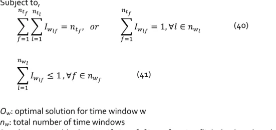
The optimal solution is the one that will allow for all the scheduled flights to be performed, using a different aircraft, and having the highest revenue (or minimum loss). The mathematical formulation:

𝛰_𝑤 = max (∑ ∑ 𝐼_𝑤𝑙𝑓∙ 𝑆_𝑤𝑙𝑓 𝑛_𝑤𝑓 𝑓=1 𝑛_𝑤𝑙 𝑙=1 ) , ∀𝑡 ∈ 𝑛_𝑡 (39)

Subject to, ∑ ∑ 𝐼𝑤𝑙𝑓 𝑛_𝑡𝑙 𝑙=1 𝑛_𝑡𝑓 𝑓=1 = 𝑛𝑡𝑓,⁡⁡⁡𝑜𝑟⁡⁡⁡⁡⁡⁡⁡⁡⁡⁡ ∑ 𝐼𝑤𝑙𝑓 𝑛_𝑡𝑓 𝑓=1 = 1, ∀𝑙 ∈ 𝑛𝑤𝑙 (40) ∑ 𝐼𝑤𝑙𝑓 ≤ 1 𝑛_𝑤𝑙 𝑙=1 , ∀𝑓 ∈ 𝑛𝑤𝑓⁡ (41)

Ow: optimal solution for time window w nw: total number of time windows

𝐼_𝑤𝑙𝑓: binary variable that is: 1 if aircraft f is performing flight leg l, and 0 otherwise

Constrain (40) ensures that all the flights included in the time window will be performed. Constrain (41) ensures that each aircraft is performing no more than one flight.

‐ Heuristic Algorithm

Algorithm (39) finds the optimal solution analytically, by testing all the possible combinations. Nevertheless, during the implementation of the model, it was noticed that for a large number of available aircraft (>11) computational time for finding the optimal solution became significantly long. For this reason, a second, heuristic algorithm was developed, that is put in use in the case that the available aircraft for the time window under examination are more than 11.

The algorithm starts by finding the highest value in the table and assumes that that pairing will be included in the optimal combination. Subsequently, it finds the next highest value in the table, complying with the constrains, and assumes the second pairing of the combination. The process is repeated until each flight is paired with an aircraft.

For better approximation to the real optimal solution, the process is iterated by starting from the second highest value, third, etc.

An example of the process showing the first two iterations is illustrated in Figure 3.

1 2 3 Α B C 25 30 15 20 10 35 40 25 15 1 2 3 Α B C 25 30 15 20 10 35 40 25 15 1 2 3 Α B C 25 30 15 20 10 35 40 25 15 1 2 3 Α B C 25 30 15 20 10 35 40 25 15 1 2 3 Α B C 25 30 15 20 10 35 40 25 15 1 2 3 Α B C 25 30 15 20 10 35 40 25 15

1

2

5.4. Post-processing

5.4.1. Aircraft Related Data Registration This step includes the following:

‐ Engine Cycles and Flight Hours Registration

The model assumes that the suggested solution has been utilized. Therefore, the record of each aircraft that has performed a flight in the given time window is being updated with the equivalent flight hours and engine cycles. Aircraft that perform a landing during the given time window at the station under examination are also taken into account.

‐ Aircraft Maintenance Registration

In order to keep track of the maintenance cycles without needing to add data manually, the model identifies the aircraft that need to undergo maintenance, and registers a maintenance cycle at the specific aircraft.

The above are modeled as follows: 𝐻_𝑚𝑖𝑓 𝑡+ = (𝐼𝑙∙ 𝑀𝑚𝑖𝑓+ 1) ∙ (𝐻𝑚𝑖𝑓𝑡−− 𝐼𝑙𝑓_𝑡𝑑 ∙ 𝐷𝑙_𝑡𝑑) + 𝐼𝑙∙ 𝑀𝑚𝑖𝑓∙ 𝐻𝑚𝑖𝑓, ∀⁡𝑡𝑑 ∈ [𝑡 −_{, 𝑡}+_{] (42)} 𝐸𝐶𝑓_𝑡+ = (𝐼𝑙∙ 𝑀𝑚𝑖𝑓+ 1) ∙ (𝐸𝐶𝑓𝑡− + 𝐼𝑙𝑓_𝑡𝑑) , ∀⁡𝑡𝑑 ∈ [𝑡−, 𝑡+] (43) 𝑀𝐶_𝑓 𝑡+ = 𝑀𝐶𝑓𝑡−+ 𝐼𝑙∙ 𝑀𝑚𝑒𝑓, ∀⁡𝑡𝑑 ∈ [𝑡 −_{, 𝑡}+_{] (44)} Where,

𝐻𝑚𝑖𝑓_𝑡+: remaining hours until the next type i scheduled maintenance for aircraft f at the end t

+ _{of time}

window w

𝐻𝑚_𝑖𝑓𝑡−: remaining hours until the next type i scheduled maintenance for aircraft f at the beginning t

of time window w

Iw: binary variable that is: 1 if time window w is the last of the day and 0 otherwise

𝑀_𝑚𝑖𝑓: binary variable that is: 1 if aircraft f needs to undergo type i maintenance at the end of the day, and 0 otherwise

𝐼_𝑙𝑓

𝑡𝑑: binary variable that is: 1 if aircraft f is performing flight leg l that departs at td and 0 otherwise

𝐷_𝑙

𝑡𝑑: duration of flight leg l departing at td (σε hr)

𝐻_𝑚𝑖𝑓: type i maintenance of aircraft f (in hr)

𝐸𝐶𝑓𝑡−: flight cycles of aircraft f, at the beginning of time window

𝐸𝐶_𝑓

𝑡+: flight cycles of aircraft f, at the end of time window

𝑀𝑚𝑒𝑓: binary variable that is: 1 if aircraft f needs to undergo engine maintenance at the end of the day and 0

otherwise

𝑀𝐶_𝑓𝑡−: engine maintenance cycles of aircraft f at the beginning of the time window 𝑀𝐶𝑓_𝑡+: engine maintenance cycles of aircraft f at the end of the time window

Equation (42) deals with registering the flight hours to aircraft that have performed a flight, or restores the available flight hours to the maximum number, if the aircraft has undergone maintenance.

Equation (43) registers aircraft engine cycles, or resets them in case the engine has undergone maintenance.

Equation (44) registers maintenance cycles, in case the aircraft has undergone maintenance.

It is important to state that the last moment of the time window is the same as the first moment of the next time window, meaning

𝑡𝑤+ ≡ 𝑡𝑤+1− (45)

5.4.2. Available Aircraft List for Next Time Window

This list consists of aircraft that have landed at the station under examination during previous time window(s), and aircraft that had been available during the previous time window, but were not assigned a flight. For the aircraft that landed during previous time windows, it is essential that enough time has passed so they can be ready for the next flight (the turn time usually takes 30-45 minutes).

The list is generated as follows: [𝐹_𝑠𝑓

𝑡+] = [𝐹𝑠𝑓𝑡−] ∙ (𝐼𝑙𝑓_𝑡𝑑 + 1) + [𝐹𝑓] ∙ (𝐼𝑠𝑎𝑓𝑡𝑎) , ∀⁡𝑡𝑑 ∈ [𝑡−, 𝑡+], 𝑠𝑎 ≡ 𝑠 (46)

Where, [𝐹_𝑠𝑓

𝑡+]: matrix that includes the available aircraft at station s, at the beginning of the time window

[𝐹𝑠𝑓𝑡−]: matrix that includes the available aircraft at station s, at the end of the time window [Ff]: matrix that includes all the aircraft in the fleet of the company under examination

𝐼_{𝑠𝑎𝑓𝑡𝑎}: binary variable that is: 1 if the flight arriving at station s at time t is performed by aircraft f, and 0 otherwise

6. MODEL IMPLEMENTATION

In order to verify its validity, the model was realized, and various cases were studied. 6.1. Assumptions

Due to the complexity of the problem, the following assumptions were made during the implementation of the model.

‐ Crew Coverage

We assume that there will always be enough crew members at the station under examination. ‐ Static En Route Charges

Although En Route charges are different for each state airspace (FIR), a static fee per flown km is considered, in order to minimize the calculations. This has an almost inconsiderable effect on the final decision. In order to minimize the error, the static en route fee is taken as the average fee per flown km of the flight region of the airline under examination.

‐ Hub-and-spoke Network

As the model performs optimization from a specific station, a hub-and-spoke network is assumed. ‐ Back-up aircraft

We assume that one back-up aircraft of each fleet type is kept at the central station. 6.2. Test Case

6.2.1. Data

The proposed algorithm was tested on a case, using an existing operational airline and its itineraries. The fleet of the airline under consideration consisted out of a total of 29 aircraft of 3 different types. The airline flies to a total of 75 destinations, most of which are in Europe.

For the needs of passenger demand forecasting, the three previous years were taken into consideration. The optimization was performed for a whole day (24 hours) with a 15 minute time window.

6.2.2. Results

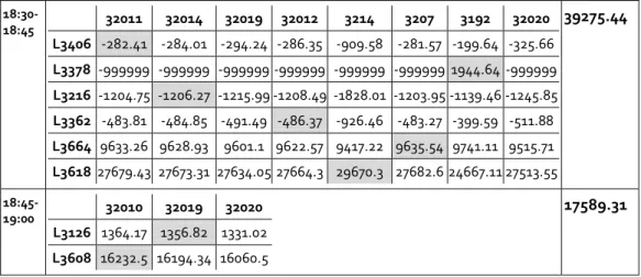
18:30-18:45 32011 32014 32019 32012 3214 3207 3192 32020 L3406 -282.41 -284.01 -294.24 -286.35 -909.58 -281.57 -199.64 -325.66 L3378 -999999 -999999 -999999 -999999 -999999 -999999 1944.64 -999999 L3216 -1204.75 -1206.27 -1215.99 -1208.49 -1828.01 -1203.95 -1139.46 -1245.85 L3362 -483.81 -484.85 -491.49 -486.37 -926.46 -483.27 -399.59 -511.88 L3664 9633.26 9628.93 9601.1 9622.57 9417.22 9635.54 9741.11 9515.71 L3618 27679.43 27673.31 27634.05 27664.3 29670.3 27682.6 24667.11 27513.55 39275.44 18:45-19:00 32010 32019 32020 L3126 1364.17 1356.82 1331.02 L3608 16232.5 16194.34 16060.5 17589.31

Table 9: Consecutive time windows modeling

The first column shows the time window under examination.

The second column includes the table with flights that need to performed, and the available aircraft for the time window. The flights are listed by their code (e.g.L3664) while for the aircraft, the first 3 digits indicate the A/C type, while the last indicate the serial number of the specific type, in the fleet (e.g. 32019 shows that it is the 19th Airbus A320 in the fleet).

The last column shows the generated profit if the optimized solution is utilized. The highlighted cells indicate the optimal combination.

The large negative numbers (-999999) in some cells indicate that the combination is not possible due to non-compliance with one or more of the restrictions mentioned in paragraph 4.1.

The negative numbers in the cells indicate that the flight is not profitable because of low passenger demand.

One can also notice that for the second time window shown in Table 9, the available A/C are the ones that were not assigned a flight during the previous time window (32019, 32020) plus the ones that landed at the station previously, and are available now (32010).

The optimal solution proposed by the model suggests 25% higher revenues than the worst possible solution for the same day.

6.3. Sensitivity Analysis

In order to study the fluctuation of the various parameters on the final solution, a sensitivity analysis was conducted. A total of 8 different parameters were studied. In order to reach objective results, 11 different flight legs and 3 different fleet types were taken into consideration.

Below the most interesting results are listed. 6.3.1. Passenger Demand

Since passenger fares are the only source of revenue for commercial flights, passenger demand plays an important role on the final decision.

In order to study the effects of passenger demand on the total revenues, a usual previous years’ demand for the flight under consideration is taken, and fluctuations of 30% around that value were examined.

Figure 4 illustrates the effects of passenger demand on the total revenues for 3 different fleet types.

The gradient change depicts the full capacity of each fleet type, namely Airbus A319, A320, A321. Above that, revenues from recaptured passengers are taken into consideration, and not actual passengers.

It is also interesting to notice that for low number of passengers, smaller fleet types, yield higher revenue, as they have lower operational expenses (airport charges, navigation charges, fuel expenses, etc.)

Figure 4: Total revenues vs passenger demand

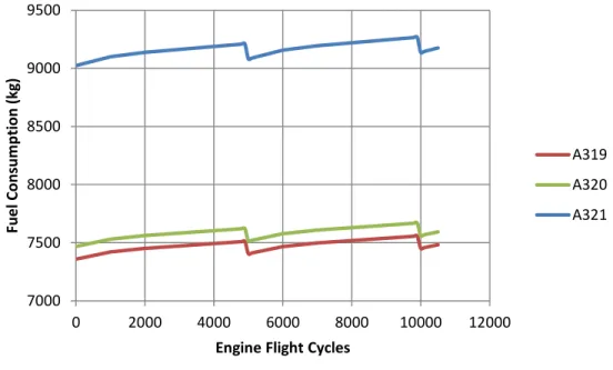
6.3.2. Engine Flight Cycles

Aircraft, and especially engine maintenance has a high impact on the fuel consumption, and subsequently on the fuel expenses.

Figure 5 illustrates the effects the impact of engine’s flight cycles (EFC) on the fuel expenses, for 3 different fleet types.

Figure 5: Fuel consumption vs EFC

One can see the engine maintenance periodicity which happens every 5000 flight cycles.

It is also visible that after each maintenance cycle the fuel consumption is not reduced to the same value for zero flight cycles. This indicates the remaining engine deterioration due to aging.

0 2000 4000 6000 8000 10000 12000 -40% -30% -20% -10% 0% 10% 20% 30% 40% To tal R e ve n u e s ( € ) Δ(Passenger Demand) A319 A320 A321 7000 7500 8000 8500 9000 9500 0 2000 4000 6000 8000 10000 12000 Fue l Co n sum p ti on (kg )

Engine Flight Cycles

A319 A320 A321

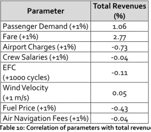
Table 10 illustrates the effects of the fluctuation of the various parameters on the total revenues.

Parameter Total Revenues (%) Passenger Demand (+1%) 1.06 Fare (+1%) 2.77 Airport Charges (+1%) -0.73 Crew Salaries (+1%) -0.04 EFC (+1000 cycles) -0.11 Wind Velocity (+1 m/s) 0.05 Fuel Price (+1%) -0.43

Air Navigation Fees (+1%) -0.04

Table 10: Correlation of parameters with total revenues

6.3.3. Optimal Solution Algorithm

In order to check the validity of the secondary proposed heuristic algorithm, a number of different cases was tested.

Specifically, more than 50 different cases were tested, with the possible pairings varying from 4 to 144. The deviation from the solution found with the analytical algorithm varies from 0% to 7% for the different cases, while the average deviation of the total of the cases tested is around 2.5%.

The deviation was found to be rather random, and not depended on the number of possible combinations. The deviation depicted from the above test cases is an acceptable error, for the benefits that the heuristic algorithm offers.

Specifically, on a notebook running on Intel 1.8 GHz Core i5 and 4GB DDR3 RAM at 1600MHz, the analytical algorithm would need around 20’’ for 12 available aircraft, around 2’20’’ for 13 available A/C, and more than 60’ for 14 available A/C.

The heuristic algorithm would need less than 1’’ for available A/C less than 15, while the computational time does not increase a lot for more A/C.

Combining the two algorithms (the secondary algorithm is put in use when the number of available A/C is more than 11) the same computer needs around 10’’ for a whole day optimization.

7. EPILOGUE 7.1. Summary

A generalized model and solution for the fleet assignment problem has been described above.

The proposed method includes modeling of restrictions on flight leg-aircraft pairing, modeling of financial figures, and suggestion of the optimal pairing for profit maximization.

The modeled restrictions include airport, aircraft and code sharing partners restrictions.

Airport restrictions include runway length checks according to ambient characteristics, noise emission checks according to timing, and aircraft ownership restrictions.

The financial figures that are being modeled are passenger revenues, fuel, airport, crew, and air navigation expenses.

Passenger revenues include passenger demand forecasting based on data from previous years, and revenues modeling based on passenger class.

Fuel expenses modeling considers fuel consumption based on engine deterioration, aircraft weight, wind velocity, and fuel price at each station, while a five stage mission analysis is used.

Airport expenses include aircraft and passenger charges considering passenger and flight type.

The optimal solution suggestion considers maintenance routing in order to minimize maintenance expenses.

The model can be used both for time period, and whole day optimization, using discrete time windows. Consecutive time windows “communicate” with data that are transferred from the end of one to the next. This gives the model the “continuity” characteristic, meaning that it can perform optimization of consecutive time windows, or days, without the need for external input.

For validation purposes, the model was realized, and a case study of an operational international airline was implemented, using the optimization software that was developed.

For sensitivity analysis purposes, more than 900 unique cases were tested, in order to study the effect of the various parameter fluctuations on the total revenues for each pairing.

7.2. Conclusion

The most notable weakness of the majority of the FAP models lie on the fact that they don’t include detailed and precise modeling of the financial figures related to each specific flight leg.

Attempting to solve this problem, a solution that integrates modeling and optimal solution suggestion into one single model which can perform optimization of consecutive time windows without the need for manual data input has been introduced.

Furthermore, some of the parameters considered by the model and neglected by many of the prevalent models have an impact on the final decision. Specifically, the consideration of engine deterioration and aircraft weight has a high impact on the fuel consumption, hence, fuel expenses, especially for longer flight legs.

Also, fleet assignment considering maintenance routing can totally change the available aircraft at different stations in the network, and radically reduce maintenance expenses.

7.3. Future Research

The following steps for further research and development of the model are proposed: ‐ Extension on Full Network

The model is ideal for hub-and-spoke networks, but its advantages are not fully utilized when the connections with the central station are loose, or there is no central station.

In order to overcome this disadvantage, an extension of the calculations is proposed, so that for each time window, an optimization of the whole of flights departing from each station in the network is performed, and not just from a specific station.

‐ Iterative Optimization over a Set of Time Windows

Although the model suggests the optimal solution for each time window, this does not guarantee the optimal solution over a set of time windows, e.g. a whole day. This happens because although the utilized fleet assignment of one time window affects all the solutions in the following time windows, the proposed approach does not consider changes in the solutions proposed for previous time windows.

In order to eliminate the above weakness, a modeling of all the possible combinations happening in a set of time windows would be necessary.

The computational time needed to perform the above calculations would be significantly larger than the one needed for the existing model because of the non-linearity of the problem. Nevertheless, techniques could be used to reduce the computational time, such as modeling of specific high traffic time windows, etc. ‐ Integration of Diagnostic Methods

In order to model fuel expenses, engine deterioration in relation with engine flight cycles is estimated. This implies a number of assumptions which imply inaccuracies in our estimations.

Using onboard measuring instruments, and relating the measurements to real engine state, a much more accurate knowledge on engine deterioration would be possible, and thus, higher accuracy on fuel consumption modeling.

Using diagnostic methods could also lead to better maintenance planning and routing. ‐ Integration of Prognostic Methods

The next step after integrating diagnostic methods would be to use prognostic methods. This way, a forecasted engine state at a point in the future would be possible. Integrating such methods could lead to minimize maintenance expenses through optimizing maintenance routing and frequency.

8. BIBLIOGRAPHY

Abara, Jeph. "Applying Integer Linear Programming to the Fleet Assignment Problem." Interfaces 19, no. 4 (1989): 20-28.

Aircraft Owner's & Operator's Guide. "CFM56-3 Maintenance Analysis & Budget." Aircraft Commerce, April/May 2006.

Barnhart, C., T. S. Kniker, and M. Lohatepanont. "Itinerary-Based Airline Fleet Assignment." Transportation

Science 36, no. 2 (May 2002): 199-217.

Barnhart, Cynthia, Peter Belobaba, and Amedeo R. Odoni. "Applications of Operations Research in the Air Transport Industry." Transportation Science 37, no. 4 (November 2003): 368-391.

Belanger, Nicolas, Guy Desaulniers, Francois Soumis, and Jacques Desrosiers. "Periodic Airline Fleet Assignment with Time Windows, Spacing Constraints, and Time Dependent Revenues." European

Journal of Operational Research, 2006: 1754-1766.

Boeing. Airports with Noise and Emissions Regulations. n.d.

http://www.boeing.com/commercial/noise/list.html.

Castelli, Lorenzo, and Andrea Ranieri. "Air Navigation Service Charges in Europe." University of Trieste, Trieste, n.d.

Civil Aviation Safety Authority. "Standard Passenger and Baggage Weights." Civil Aviation Advisory

Publication. September 1990.

Clarke, L. W., C. A. Hane, E. L. Johnson, and G. L. Nemhauser. "Maintenance and Crew Considerations in Fleet Assignment." Transportation Science 30, no. 3 (August 1996): 249-260.

Embraer. "Takeoff Runway Length Adjustment." Airport Planning Manual. n.d. Eurocontrol. Base of Aircraft Data. n.d. http://www.eurocontrol.int/services/bada.

European Parliament. "Directive 2008/101/EC of the European Parliament and of the Council so as to Include Aviation Activities in the Scheme for Greenhouse Gas Emmision Allowance Trading Within the Community." Official Journal of the European Union, November 2008: 8/3-8/21.

ICAO. Noise Certification Database. September 13, 2012. http://noisedb.stac.aviation-civile.gouv.fr/results.php.

Kelaidis, M., N. Aretakis, A. Tsalavoutas, and K. Mathioudakis. "Optimal Mission Analysis Accounting for Engine Aging and Emissions." Journal of Engineering for Gas Turbines and Power 131 (January 2009). Lapp, Marcial, and Amy Cohn. "Modifying Lines-of-flight in the Planning Process for Improved Maintenance

Robustness." Computers & Operations Research, 2012: 2051-2062.

Rexing, Brian, Cynthia Barnhart, Tim Kniker, Ahmad Jarrah, and Nirup Krishnamurthy. "Airline Fleet Assignment with Time Windows." Transportation Science, no. 34 (2000): 1-20.

The Guides Network. n.d. http://www.world-airport-codes.com.

Walid, El Moudani, and Mora-Camino Felix. "A Dynamic Approach for Aircraft Assignment and Maintenance Scheduling by Airlines." Journal of Air Transport Management, 2000: 233-237.

Walpole, Sarah Catherine, David Prieto-Merino, Phil Edwards, John Cleland, Gretchen Stevens, and Ian Roberts. "The Weight of Nations - An Estimation of Adult Human Biomass." Public Health, 2012.

Yaworski, Michael J., Eric P. Dinges, and Ralph J. Iovinelli. "High-Fidelity Weather Data Makes a Difference Calculating Environmental Consequences with FAA’s Aviation Environmental Design Tool." Ninth