Spectral-Spatial Classification Integrating Band
Selection for Hyperspectral Imagery
With Severe Noise Bands
Ji Zhao
, Suzheng Tian, Christian Geiß
, Member, IEEE, Lizhe Wang
, Yanfei Zhong
, Senior Member, IEEE,
and Hannes Taubenböck
Abstract—Spectral-spatial classification for hyperspectral im-agery has been receiving much attention, since the detailed spectral and rich spatial information of hyperspectral images can be fully exploited to improve the classification accuracy. However, when the original hyperspectral images have very noisy bands, these bands may have an unfavorable impact on the classification, and are often discarded in advance based on expert knowledge. In this study, a spectral-spatial conditional random field classification algorithm integrating band selection (CRFBS) is developed for hyperspectral imagery with severe noise bands. The proposed algorithm inte-grates band selection based on the relative utility of the spectral bands for classification. Consequently, negative effects of severe noise bands are eliminated and the need for high-quality image data is substantially reduced. In addition, the CRFBS algorithm makes comprehensive use of both the spectral and the spatial cues to improve the classification performance. The spectral cues are formulated by integrating the support vector machine and random forest algorithms to improve the spectral discriminative ability in the unary potentials, and the spatial information are modeled to consider the interactions between pixels in pairwise potentials. The experiments using different airborne and UAV-borne hyperspectral data verified the effectiveness of the CRFBS method. The CRFBS algorithm can achieve accurate interpretation of the various clas-sification categories and a more than 3% improvement in classi-fication accuracy, compared with the method using the original hyperspectral image with severe noise bands.
Index Terms—Conditional random fields, hyperspectral image, image classification, random forest, spectral-spatial classification.
Manuscript received January 22, 2020; revised March 6, 2020; accepted March 17, 2020. Date of publication April 13, 2020; date of current version April 30, 2020. This work was supported in part by the National Natural Science Foundation of China under Grant 41801280, Grant U1711266, Grant 41925007, and Grant 41771385, and in part by the Fundamental Research Funds for the Central Universities, China University of Geosciences (Wuhan) under Grant CUG170676. (Corresponding author: Lizhe Wang.)
Ji Zhao is with the School of Computer Science, China University of Geo-sciences, Wuhan 430074, China, and also with the German Aerospace Center (DLR), German Remote Sensing Data Center (DFD), 82234 Oberpfaffenhofen, Germany (e-mail: [email protected]).
Suzheng Tian and Lizhe Wang are with the School of Computer Sci-ence, China University of Geosciences, Wuhan 430074, China (e-mail: [email protected]; [email protected]).
Christian Geiß and Hannes Taubenböck are with the German Aerospace Center (DLR), German Remote Sensing Data Center (DFD), 82234 Oberp-faffenhofen, Germany (e-mail: [email protected]; Hannes.Taubenboeck @dlr.de).
Yanfei Zhong is with the State Key Laboratory of Information Engineering in Surveying, Mapping and Remote Sensing, Wuhan University, Wuhan 430079, China (e-mail: [email protected]).
Digital Object Identifier 10.1109/JSTARS.2020.2984568
I. INTRODUCTION
H
YPERSPECTRAL imagery is a very important data source for deriving detailed thematic information on the earth surface, since it contains hundreds of narrow spectral channels to distinguish the subtle spectral difference of various materials [1], [2]. Therefore, hyperspectral image classification is an enduring research topic [3]. Hyperspectral image clas-sification aims at labeling each pixel with specific semantic categories, and can be used for manifold applications [4], such as precision agriculture, mineral mapping, or environmental monitoring. However, in the classification process there is a strong correlation between hundreds of narrow spectral bands, which results in redundant information content and high spectral dimensionality. This can lead to a high-dimensional processing problem, the so-called Hughes phenomenon [5], if only a limited number of training samples are available.To solve high-dimensional problems in hyperspectral im-age classification when the samples cannot be significantly increased, there are two options: first, to reduce the dimension of the hyperspectral data, and second, to improve the process-ing capability of classifiers that use high dimensional features. Dimensionality reduction can be achieved by band selection or feature extraction to solely retain useful information [6]. Feature extraction creates new features in a feature space with lower dimensionality while satisfying certain criteria regarding the original spectral features [7], [8]. Such techniques comprise linear discriminant analysis and principal component analysis, among others. In contrast, band selection is to select representa-tive band subsets from the original spectral channels to preserve important information and reduce the number of bands [9], [10]. Examples are the band selection method based on saliency bands and scale selection (SBSS) [11] and the salient band selection method based on manifold ranking [12].
For classification, there are methods that have the ability to deal with the problem of learning a robust model from a high-dimensional feature vector in conjunction with limited training samples. Support Vector Machine (SVM) and Random Forest (RF) are typical classification algorithms, which have received extensive attention in hyperspectral classification [13], [14]. SVM is a discriminative classifier to find a decision bound-ary that effectively separates different classes. The decision boundary is a separating hyperplane formed by support vectors,
and can distinguish complex two-class scenes based on the kernel technique [15]. Among numerous supervised pixel-wise image classification algorithms (such as neural network and RF methods), SVM is considered to achieve the highest accuracy [16]. However, RF is a typical ensemble learning algorithm to combine multiple decision tree classifiers to achieve a stable and better classification performance compared to individual models. RF randomly selects spectral feature subsets, and is insensitive to data with some missing features as well as noisy features. More importantly, RF can not only handle classification problems with high-dimensional feature spaces like SVM, but it also allows for interpretability by enabling to estimate which variables play an important role in the classification. Therefore, RF is widely used in image classification [13], and has a series of extended models, such as rotation forest [17], [18], among others. These pixel-wise classification algorithms process each pixel independently based on spectral information without con-sidering spatial correlation between pixels, and always have obvious salt-and-pepper classification results which affect clas-sification accuracy negatively.
To improve classification performance, spatial information of hyperspectral imagery can be additionally exploited. The spectral-spatial classification approaches comprehensively uti-lize spectral and spatial information to help accurately recognize semantic categories [19], and lots of spectral-spatial classifi-cation algorithms have been developed [3], [20], [21]. Object-oriented and deep learning approaches have often been applied. For the object-oriented classification, it takes objects as the pro-cessing unit [22]–[25] to consider the spatial information. The objects are first generated by segmentation, such as the fractal net evolution approach (FNEA) [26]. The object features obtained from spatial statistics of pixels in an object can be used to enable final classification results. A majority voting strategy within each object is another way to obtain the labels using pixel-wise classification [27]. For spectral-spatial methods based on deep learning, the approach can mine the spatial structure information of the images by a designed network structure [28]–[30]. For example, as an effective deep learning model, convolutional neural network (CNN) is mainly composed of a series of con-volution and pooling layers to extract effective spatial structure features, and uses a stack of fully connected layers to perform the classification tasks [31]. Combining the characteristics of hyperspectral remote sensing images, CNN has developed a number of models for hyperspectral classification task [30], such as the spectral-spatial attention network with an attention mechanism [32] and spectral-spatial residual network using 3-D convolutional layer [33]. These CNN classification frameworks can achieve good classification performance. However, these classification models based on deep learning often require a large number of training sets to optimize a mass of parameters in the network structure.
Beyond that, the random field model is another method to explicitly model spatial information by constructing the corre-spondence between images and graphs. The Markov random field and conditional random field (CRF) models are widely used random field models in image processing [34]–[36]. For hy-perspectral image classification, multiple research works about
random fields have been carried out to deal with specific issues. For example, a spectral-spatial classification method using CRF and active learning was proposed to use spatial and spectral information to enlarge the training set efficiently [37]. The rotation forests with local feature extraction was used to model the potential functions of MRF to improve classification accu-racy [17]. A spectral-spatial classification method inspired by game theory was developed to use a cooperative game to obtain final classification results [38]. These classification algorithms achieve good classification performance by considering the spatial information, compared to pixel-wise classification algo-rithms. However, they often depend on the ability of potential functions to model the relationship between classification labels and the hyperspectral image, and are sensitive to the quality of hyperspectral data. The input original hyperspectral image often have very noisy bands, and may even have bands which carry solely zero values and do not contain any useful information. These noise bands, such as water absorption bands, have a certain impact on classification, and are often removed in advance based on expert knowledge.
In order to mitigate the effect of noise bands and to improve the robustness of the random field model for hyperspectral data, we develop a spectral-spatial conditional random field classification algorithm integrating band selection (CRFBS) for hyperspectral imagery with severe noise bands. In the CRFBS algorithm, the potential functions are used to model the posterior probability to achieve the classification labels, which depend on the quality of hyperspectral data. Accordingly, the band selection based on the relative utility of the spectral bands is proposed to provide ideal data. The traditional band selection method selects information metrics independent of classification tasks, such as information gain, which may not be able to improve classification perfor-mance. In contrast, the proposed band selection method selects the relative importance of the spectral bands as an effective measure to select important bands, which is directly related to the classification task and can be used to distinguish the various classes. To alleviate the uncertainty between spectrum and category mapping, the selected bands with greater impact on classification and spatial contextual information are exploited by potential functions of CRF model to improve the classification performance. The unary potential is formulated by the class membership probabilities to provide the basic discriminative information of various semantic classes based on the spectral cues, and the pairwise potential models the spatial interactions between image pixels to favor the homogenous regions of a hyperspectral image take the same classification label in the classification map. In summary, the main contributions of this work are as follows: (1) the band selection based on the relative utility of the spectral bands is developed to select the important bands. (2) The band selection is integrated in the CRFBS algo-rithm to automatically alleviate the effects of severe noise bands. (3) Both the spectral and the spatial cues are exploited based on potential functions of the CRF model to improve classification performance.
The effectiveness of the CRFBS algorithm was tested using different hyperspectral datasets with some bands contaminated with severe noise, and the experimental results showed that the
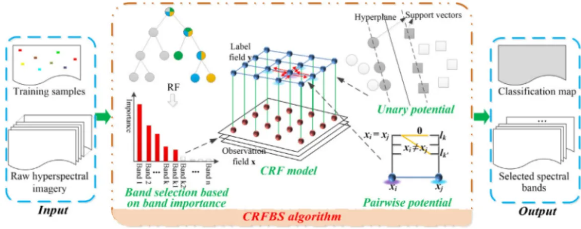
Fig. 1. Framework of the spectral-spatial conditional random field classification integrating band selection (CRFBS).
CRFBS method has a competitive classification performance, compared with other state-of-the-art hyperspectral image clas-sification approaches.
In the rest of this paper, we describe the proposed CRFBS algorithm in Section II, present the used experimental data (Section III), show the corresponding experimental results in Section IV, give several necessary analysis for the proposed algorithm (Section V) and draw conclusions in Section VI.
II. PROPOSEDCRFBS METHOD
To eliminate the effects of severe noise bands, the CRFBS algorithm is proposed in this section. As shown in Fig. 1, the CRFBS approach contains four main interlinked modules: (1) the core CRF model is constructed to provide spectral-spatial classification framework. (2) The band selection based on band importance measure selects the spectral bands useful for classi-fication by sorting the importance of each band to obtain ideal observation data for CRF model. (3) The unary potential models the relationship between classification labels and observation data by the class membership probabilities, which is obtained by non-linear SVM. (4) The pairwise potential models the spatial interactions of neighboring pixels to encode the spatial patterns of classification classes. These modules are detailed in the following four subsections.
A. CRF Framework
The classification of hyperspectral images aims to find the op-timal pixel label using known spectral cues of the image, and can be considered as maximizing a posteriori probability of the cate-gory labels using the input hyperspectral image. As a widely used probabilistic graphical model, CRF attempts to directly model a
posteriori probability to consider the spatial information using
the correspondence between images and graphs [36]. Consider an original input hyperspectral imagex={x1,x2, . . . ,xN}, wherexirepresents the spectral values of image pixeli∈V = {1,2, . . . , N}, and N is the number of pixels. The classification label can be denoted asy={y1, y2, . . . , yN}, where each label
yi of image pixel i takes a value from the label set L={1, 2, … ,K}, and K is the number of classes. Thereby, CRF can use a
Gibbs distribution to model a posteriori probability [39]:
P(y|x) = 1 Zexp − c∈C ψc(yc,x) (1) where Z represents the partition function.ψc(yc,x)is called the potential function and is a positive function of random variables in the clique c, which can be divided into unary, pairwise, and even higher-order potential functions according to the different types of cliques. Considering the inference difficulty for a gen-eral higher-order potential function, the CRF including unary and pairwise potential functions is widely used:
P(y|x) = 1 Zexp ⎧ ⎨ ⎩− i∈V ψi(yi|x)−λ i∈V,j∈Ni ψij(yi, yj|x) ⎫ ⎬ ⎭ (2)
whereψi(yi|x)andψij(yi, yj|x)represent the unary potential term and pairwise potential term to model the dependencies of pairs of random variables, respectively.Niis the local neighbor-hood of pixel i, and 8-neighborneighbor-hood connectivity is widely used to encode the spatial-contextual relationship [40].λcontrols the strength of the pairwise potential term relative to the unary po-tential term. The posteriori probability based on (2) is converted to the corresponding Gibbs energy:
E(y|x) =−log (P(y|x))−log (Z) = i∈V ψi(yi|x) +λ i∈V,j∈Ni ψij(yi, yj|x). (3)
It can be seen that the classification problem can minimize equivalently the energy function E(y|x) to obtain the optimal classification label y. To minimize the energy function, we apply the graph-cut inference algorithm [41] in our study, as it is considered an efficient approximation method.
The general CRF framework is established for hyperspectral image classification, and the remaining problem is to formulate unary and pairwise potential terms. Based on (3), the unary and pairwise potential functions can be considered to depend on the input hyperspectral image x. Accordingly, the noisy bands in
the input original hyperspectral image will affect the effective construction of these potential functions and have a further impact on the spectral-spatial classification performance. To eliminate the effects of the noisy bands, the band selection based on the relative importance is integrated in the CRF framework and is also introduced in the following subsection.
B. Band Selection Based on Band Importance Measure
Hyperspectral images often have many spectral bands, which have different discriminative capabilities for distinguishing clas-sification categories because they are in the different parts of the spectrum [42]. Some bands that are more useful for distinguish-ing categories have greater importance. Some bands contain severe noise and even have no information value, so they have no positive effect on classification. In this study we develop band selection based on band importance measure to eliminate the effects of severe noise bands and select useful bands for classification. The importance of the bands is first obtained, and then the spectral bands with high importance are selected based on the given cumulative band importance keeping ratio.
To measure band importance, we apply the RF classification method, which is a widely used ensemble algorithm. The RF algorithm was proposed to overcome the overfitting problem of decision trees based on the aggregation of multiple decision trees, i.e., bagging [43]. It has an excellent performance in hy-perspectral classification [13], [44], [45] due to its high- dimen-sional data processing capabilities. Another potential feature of RF algorithms is the ability to measure relationships between input features and output variables, which is denoted as variable importance. The variable importance in the RF method can be calculated based on the average value of cumulative reduction in node impurity for all the trees of the ensemble. Accordingly, the importance value of a variable Xmis calculated by averaging the sum of the weighted node impurity reductions of all nodes t using Xmover allNT trees in the forest for estimating Y.
Imp(Xm) = 1 NT T t∈T:v(st)=Xm p(t)Δi(st, t) (4)
where p(t) is the weight and can be calculated by the propor-tion of samples reaching node t.v(st)represents the variable used in the splitst andΔi(st, t)is the impurity reduction of the split st at node t. To select spectral bands that are useful for classification, the spectral bands of hyperspectral images are used as input variables of the RF algorithm. Accordingly, the band importance obtained by (4) can reveal the different roles of each spectral band in the classification, which can be exploited to select the spectral bands that play an important role in classification. To obtain the final spectral band set, we sort by spectral band importances in descending order, and select the spectral bands by setting a threshold of cumulative band importance keeping ratio.
Ind = argmin Ind Ind i=1 SortedImp(Xi)> B i=1 SortedImp(Xi)∗δ (5) SelBands = Xi|Imp(Xi)>SortedImp(XInd) (6)
where SortedImp(Xi) represents the sorted band importance in descending order and B is the band number of the original input hyperspectral image. (5) aims to find the first subscript Ind of the sorted band importance to satisfy the cumulative proportion of the sorted band importance is greater than the given thresholdσ. We obtain the band importance threshold based on the calculated subscript, so that we can select the spectral bands that the corresponding band importance is greater than the band importance threshold, according to (6). The top ranked bands have greater importance and play a greater role in classification, so that severe noise bands can be discarded automatically due to their lower importance.
C. Unary Potential
The unary potential function of CRF framework mainly mod-els the relationship between category labmod-els and image features, and calculates the cost of each pixel taking a classification label using the selected spectral bands. In the hyperspectral image classification tasks, the unary potential term is formulated by the class membership probabilities, which can be obtained by discriminative classifier using the selected spectral bands. Accordingly, the used unary potential is formulated as:
ψi(yi|x) =−ln (P(yi=lk|¯x)), ¯x⊆x. (7) The unary potential term of CRF uses the class membership probabilities of pixelP(yi=lk)to calculate the cost of taking class label lk at the hyperspectral image i based on the the selected spectral bands¯x. The class membership probabilities can be obtained by any discriminative classifier. In this study, the SVM with nonlinear Gaussian radial basis function (RBF) kernel is used to obtain the probability because the classification categories are not linearly separable in hyperspectral image classification and the non-linear SVM can achieve excellent classification performance using limited training samples. To obtain the class membership probabilities of SVM, the Platt’s formulation is used to give the probability estimates based on the class label outputs of SVM, which is implemented in the LIBSVM library [46]. Since the SVM algorithm is sensitive to severe noise bands, a subset of bands obtained by band selec-tion is used to exclude the interference effects of unimportant bands for hyperspectral image classification. Considering that the selected band is based on band importance measure from RF, the unary potential term can be considered to indirectly combine the advantages of the RF and SVM algorithms in the CRFBS classification framework to more accurately distinguish the different categories for hyperspectral imagery with severe noise bands.
D. Pairwise Potential
The pairwise potential function of CRF framework models the spatial interactions between pixels based on the spatial patterns of classification classes that neighboring pixels in a homogeneous area tend to take the same label. The spatial prior knowledge is of importance to help mitigate the classification uncertainty based on spectral information and alleviate the ef-fects of salt-and-pepper classification noise. Accordingly, the used pairwise potential is formulated as the following form to
encourage the neighborhood pixels of a hyperspectral image to take the same class label [40].
ψij(yi, yj|x) = ⎧ ⎨ ⎩ 0 ifyi=yj 1+θexp(−||¯xi−¯xj||2/β) ||i−j||2 otherwise (8)
The pairwise potential term of CRF models the spatial in-teraction between neighborhood pixel positions i and j of a hyperspectral image based on their spectral difference. The ¯x represents the selected subset of spectral bands.θcontrols the corresponding strength, andβcan be set to twice the mean square value of the spectral difference of all adjacent pixels in the hy-perspectral image. Based on (8), the pairwise potential term pe-nalizes the spatial inconsistencies of adjacent pixel classification categories based on the spectral difference, so that the pairwise potential term favors the homogenous regions of a hyperspectral image take the same classification label. Compared to unary potential term, the pairwise potential function considers the spa-tial patterns to eliminate the uncertainty between spectrum and class mapping by modeling the spatial interaction of neighboring pixels. Therefore, CRF can integrate the spectral and spatial information using the unary and pairwise potentials to alleviate the effects of spectral variability.
III. EXPERIMENTALDATA
In our experimental set-up, we apply three hyperspectral datasets from different experimental areas and different sen-sors to analyze the performance of the CRFBS method. These obtained hyperspectral images have some bands contaminated with severe noise, which are expected to have a certain impact on the classification accuracy. In practice, low-noise spectral bands are often used, and some severely noisy bands are removed in advance, based on expert knowledge. Considering that the pro-posed algorithm can directly deal with the original hyperspectral image with noisy bands by integrating band selection based on the relative importance of the spectral bands, the obtained raw hyperspectral data with noise spectral bands are used to verify the effectiveness of the CRFBS method.
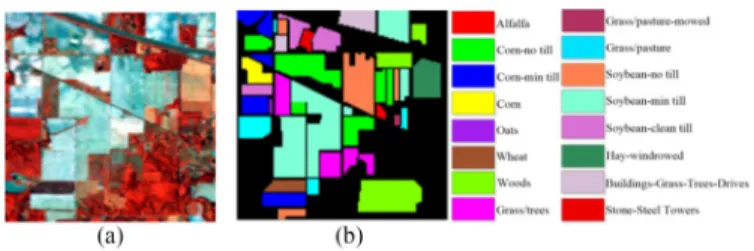
The first experimental dataset is the publicly available In-dian Pines hyperspectral data, which was acquired by the Air-borne/Visible Infrared Imaging Spectrometer (AVIRIS) sensor. The hyperspectral image contains 145×145 pixels with 20 m spatial resolution and 224 spectral channels between 0.4 and 2.5μm. However, the data we actually obtain have only 220 spectral channels, and these spectral channels are used directly in our experiments. There are 16 thematic classes in the Indian Pines dataset. The overall appearance of the experimental area and the corresponding category distribution are presented in Fig. 2(a) and (b), respectively. The detailed class information containing the number of training and test samples for the Indian Pines dataset is provided in Table I.
The Salinas hyperspectral dataset used in the second experi-ment was acquired by the AVIRIS sensor from the Salinas Valley, California. The hyperspectral image has 512×217 pixels with 3.7 m spatial resolution. The Salinas dataset originally has 224 spectral bands between 0.4 and 2.5μm, which contains 20 water
Fig. 2. Indian Pines dataset. (a) Three-band false color image. (b) Ground-truth image.
TABLE I
CLASSINFORMATION FOR THEINDIANPINESIMAGE
Fig. 3. Salinas dataset. (a) Three-band false color image. (b) Ground-truth image.
absorption spectral bands. All these spectral channels are used in our experiments, and no bands have been discarded in advance. As shown in Fig. 3, an overview and the spatial distribution of 16 agricultural types are given. In this experiment, only 15 labeled pixels for each class were selected as training samples, due to the relatively high separability between most categories of the Salinas dataset. The detailed class information used for classification is reported in Table II.
The third experimental dataset is the WHU-Hi-HanChuan UAV dataset from Hanchuan [47], Hubei province, China, which was acquired by a Headwall Nano-Hyperspec sensor mounted
TABLE II
CLASSINFORMATION FOR THESALINASIMAGE
Fig. 4. WHU-Hi-HanChuan UAV dataset. (a) Visible data and photos of the some typical crop types in the study area. (b) Hyperspectral image. (c) Ground-truth image.
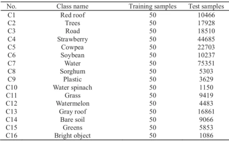
on Aibot X6 six-rotor UAV in June 2016. The acquired hyper-spectral image contains 303 × 1217 pixels and 274 spectral channels between 400 and 1000 nm with several severe noise bands. The spatial resolution of the image is 0.1 m, since the flight height of the UAV was set to 250 m. Fig. 4(a) gives an overview of this study area based on obtained visible data and some photos of the typical crop types from field investigation. The image mainly has 16 semantic classes, which were labeled in detail and cover almost the whole of the image to effectively eval-uate classification algorithms. The corresponding hyperspectral image and spatial distribution of the various categories are shown in Fig. 4(b) and Fig. 4(c). In this experiment, the numbers of training and test samples are given in Table III.
IV. RESULTS ANDANALYSIS
In this section, the experimental results using different hyper-spectral datasets are described and analyzed to test the effec-tiveness of the CRFBS algorithm. CRFBS was compared with several state-of-art classification methods, including pixel-wise, object-oriented and deep learning approaches. For the pixel-wise classification method, SVM was selected as the comparison algorithm, which uses an RBF kernel and is implemented in LIBSVM [46]. For the object-oriented classification method, a
TABLE III
CLASSINFORMATION FOR THEWHU-HI-HANCHUANUAV IMAGE
multi-resolution segmentation algorithm implemented in eCog-nition 8.0 (FNEA) was used to obtain segmentation objects, and a majority voting strategy was applied to obtain the object-oriented classification map based on the pixel-wise SVM clas-sification map. The corresponding object-oriented approach is denoted by OO-FNEA in our study. The deep learning approach used as a comparison algorithm was the spectral-spatial attention network (SSAN) [32], which extracts spectral-spatial features based on a spectral attention bi-directional recurrent neural network branch and a spatial attention CNN branch.
In addition, the band selection based on band importance is integrated in the CRFBS algorithm, which is denoted as BIBS in our study, so that the improvement of this mechanism can be evaluated. To verify that band importance can be used for feature selection, the BIBS method is compared with some state-of-art band selection approaches: the band selection method based on saliency bands and scale selection (SBSS) [11] and the supervised band selection based on modified ant lion optimizer (MALO) [48]. All bands of hyperspectral imagery are also used as a benchmark, which is denoted as AllBands. The optimal selected feature subset obtained by these band selection methods (SBSS, MALO, and BIBS) as well as all bands of the hyperspec-tral imagery are used as input to the SVM to achieve a pixel-wise classification performance.
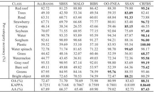
The classification maps for the various classification methods (AllBands, SBSS, MALO, BIBS, OO-FNEA, SSAN, and CRFBS) with the Indian Pines, Salinas, and WHU-Hi-HanChuan UAV datasets are shown in Figs. 5–7 respectively. They allow for a qualitative assessment of the results. To quantitatively evaluate these classification results, several common measures of classification accuracies are used, including the accuracy of each class, the overall accuracy (OA), the average accuracy (AA), and the Kappa coefficient (KAPPA). The corresponding classification accuracies are reported in Tables IV–VI for the Indian Pines, Salinas, and WHU-Hi-HanChuan UAV datasets.
For the pixel-wise classification methods (AllBands, SBSS, MALO, and BIBS), as shown in Figs. 5–7, they all present severe salt-and-pepper classification noise mainly because there is no consideration of spatial information, which can effectively
Fig. 5. Classification results for the Indian Pines dataset. (a) Ground-truth. (b) AllBands. (c) SBSS. (d) MALO. (e) BIBS. (f) OO-FNEA. (g) SSAN. (h) CRFBS.
Fig. 6. Classification results for the Salinas dataset. (a) Ground-truth. (b) AllBands. (c) SBSS. (d) MALO. (e) BIBS. (f) OO-FNEA. (g) SSAN. (h) CRFBS.
Fig. 7. Classification results for the WHU-Hi-HanChuan UAV dataset. (a) Ground-truth. (b) AllBands. (c) SBSS. (d) MALO. (e) BIBS. (f) OO-FNEA. (g) SSAN. (h) CRFBS.
TABLE IV
CLASSIFICATIONACCURACIES FOR THEINDIANPINESDATASET
TABLE V
CLASSIFICATIONACCURACIES FOR THESALINASDATASET
reduce the degree of spectral confusion between different cat-egories. These pixel-wise classification algorithms select the corresponding optimal spectral band subset based on differ-ent metrics. In consequence they have differdiffer-ent classification performances. As reported in Table IV–VI, the proposed band selection methods (BIBS) using the selected band subsets show – compared with all input bands of hyperspectral remote sens-ing images – improved classification accuracy. This is due to the capability to select more informative spectral channels to eliminate the impact of noise bands.
We find the classification accuracy of the proposed BIBS method has been improved by more than 3% compared with the use of all spectral bands. And we find these improvements for the Indian Pines, Salinas, as well as the WHU-Hi-HanChuan UAV datasets. Compared with other band selection methods (SBSS
and MALO), BIBS can achieve comparative classification per-formance, or partly even higher classification accuracy. These classification results illustrate that the band selection method based on the band importance has the capability to select a subset of spectral bands that are beneficial for classification. With it the negative effects of noise bands are lowered and thus, classification performance is improved.
For the spectral-spatial classification methods, the object-oriented approach and the deep learning algorithm deliver smoother classification results. Beyond they improve classifi-cation accuracies by considering spatial contextual information, compared with the pixel-wise approaches. As shown in Figs. 5– 7(f), the classification maps of OO-FNEA method tend to be more regular due to the constraints of segmentation results. However, it remains an unsolved challenge to select optimal
TABLE VI
CLASSIFICATIONACCURACIES FOR THEWHU-HI-HANCHUANUAV DATASET
segmentation scales [22] because of the scale diversity of the different classification types. Thus, some similar categories may be misclassified, such as the vineyard_untrained and the grapes_untrained classes in Fig. 6. The deep learning method (SSAN) exhibits better classification accuracy than OO-FNEA due to the strong learning ability and spatial information uti-lization ability of deep learning. In the case of limited training samples, the SSAN algorithm still causes confusion in some similar categories, such as corn-no till and soybean-min till categories in Fig. 5.
For the proposed CRFBS algorithm, the band selection based on the relative utility of the spectral bands is integrated to select important bands that are beneficial for classification and to alleviate the effects of input noise spectral bands. On the other hand, the spatial interactions of pixels are considered by pairwise potentials of CRF to provide the complementary information for spectral cues from the spatial dimension to improve the separability between classification categories. Accordingly, the CRFBS algorithm delivers an improved classification perfor-mance in both, the evaluation of the classification maps in a qualitative sense as well as the quantitative results. As reported in Table IV–VI, CRFBS shows better classification accuracies. And it shows an increase of more than 11% in OA over the high-est accuracy of the pixel-wise approaches for the Indian Pines, Salinas, and WHU-Hi-HanChuan UAV datasets. Compared with the spectral-spatial classification methods (OO-FNEA and SSAN), CRFBS also leads to better classification accuracies and visual results. For example, CRFBS can correctly distin-guish the vineyard_untrained and the grapes_untrained classes in Fig. 6, and shows an improvement for these classes in classi-fication maps and classiclassi-fication accuracies. Overall, we find the spectral-spatial classification methods (OO-FNEA and SSAN) can achieve reasonable classification results, and the CRFBS method exhibits a competitive classification performance for the Indian Pines, Salinas, and WHU-Hi-HanChuan UAV datasets.
V. DISCUSSION
A. Effect of Important Bands for Classification Accuracy of the SVM and RF Approaches
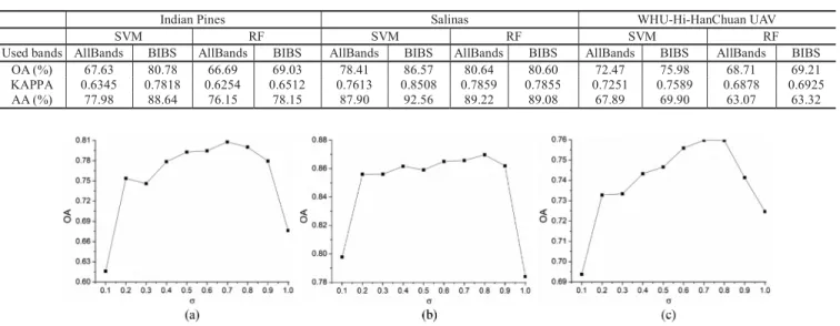
The CRFBS method integrates the band selection based on band importance to select the bands that are useful for classi-fication, and this relative utility level of the spectral channels is obtained by the RF method. The original input hyperspectral image often has noisy spectral bands, so that the classification ef-fect of important bands after removing noise bands for the SVM and RF approaches is analyzed, and the rationality of integrating these methods is explained in this section. Thereby, additional experiments were conducted using SVM and RF classifiers with all spectral bands (AllBands) and selected bands based on band importance (BIBS) for the three datasets. In the experiments, the threshold of cumulative band importance keeping ratioσis set to 0.7, and the corresponding numbers of selected spectral bands using the BIBS algorithm are 118, 103, and 164 for the Indian Pines, Salinas, and WHU-Hi-HanChuan UAV datasets, respectively. The original input spectral bands and the selected important spectral bands were used to analyze the classification effect of the important bands for the SVM and RF approaches. The classification accuracies are reported in Table VII.
From the results shown in Table VII, we draw the conclusion that SVM can achieve a higher classification accuracy when the data are ideal for hyperspectral image classification. SVM shows improvements of more than 6% over RF in OA for the three datasets using the selected important spectral bands. However, the original input hyperspectral image often contains noise bands and uninformative bands, which have a great impact on the SVM algorithm. As reported in Table VII, the SVM algorithm using selected important spectral bands has a higher classification accuracy than that achieved with the original spectral bands. The OA shows a more than 3% improvement for all three experimental data. This demonstrates that it is beneficial to select these important bands to achieve a better classification
TABLE VII
CLASSIFICATIONACCURACIES OFSVMANDRF CLASSIFIERSUSINGALLSPECTRALBANDS(ALLBANDS)ANDSELECTEDBANDSBASED ONBANDIMPORTANCE
(BIBS)FOR THEINDIANPINES, SALINAS,ANDWHU-HI-HANCHUANUAV DATASETS
Fig. 8. Sensitivity analysis for threshold of cumulative band importance keeping ratioσusing the Indian Pines, Salinas, and WHU-Hi-HanChuan UAV datasets. (a) Indian Pines. (b) Salinas. (c) WHU-Hi-HanChuan UAV.
result. Compared with the SVM approach, we find for the RF algorithm a relatively small impact on classification accuracy us-ing the important bands after removus-ing noise bands. Therefore, to obtain a better classification performance, the advantages of both algorithms are integrated in our research. The RF algorithm is used to select important spectral channels for original input hyperspectral image based on the utility level of the spectral bands. The SVM algorithm uses the selected spectral bands obtained by RF to improve the classification performance in the case of ideal data.
B. Systematic Threshold Analysis of Cumulative Band Importance Keeping Ratio for the BIBS Algorithm
The threshold of cumulative band importance keeping ratio
σ is an important parameter for the band selection based on band importance. This parameter is used to adjust the retention ratio of the cumulative band importance and indirectly affects the number of selected spectral bands. In this subsection, a sensitive analysis of the parameterσ for the BIBS algorithm is given, and additional experiments were conducted to analyze the classification effects using the Indian Pines, Salinas, and WHU-Hi-HanChuan UAV datasets. To analyze the effects of parameterσ, its value was systematically tested from 0.1 to 1, with an interval of 0.1. The corresponding classification accu-racies (OA) with different parameterσare given in Fig. 8.
As shown in Fig. 8, the classification accuracy is at a low level, when the parameter is set to 0.1. This is mainly because only the most important spectral bands are used for classification. Obvi-ously the reduction of spectral bands in this parameter setting is too restrictive, which results in a comparatively low classifi-cation accuracy. However, still more the 60% OA is achieved. In the initial stage when the parameterσincreases, classification accuracy increases rapidly since more useful spectral bands for
TABLE VIII
SELECTEDBANDS OFBIBSFOR THEINDIANPINES, SALINAS,AND
WHU-HI-HANCHUANUAV DATASETS
classification are selected. When parameterσreaches a certain value and most of the information bands have been selected, the classification accuracy can reach the corresponding highest value. After that, when more bands that did not have much effect on classification were added, the classification accuracy showed a decreasing trend. Overall, the threshold of cumulative band importance keeping ratioσhas a great impact on classification accuracy to select the spectral bands with different importance. However, as it can be observed from Fig. 8, we empirically find that there are basically enough important bands used for clas-sification, when the parameter is set to 0.7. The corresponding selected spectral bands are reported in Table VIII for the Indian Pines, Salinas, and WHU-Hi-HanChuan UAV datasets.
As shown in Table VIII, the selected spectral bands have many continuous intervals and the numbers of selected spectral bands are 118, 103, and 164 for the three experimental datasets, respectively. The BIBS only selects the spectral bands that are useful for classification based on band importance measures and adjacent spectral bands always have similar importance due to the correlation between the bands. Accordingly, many spectral bands in continuous intervals with the higher relative utility are
TABLE IX
CLASSIFICATIONRESULTS OFCRF USINGALLSPECTRALBANDS(ALLBANDS)
ANDSELECTEDBANDSBASED ONBANDIMPORTANCE(BIBS)FOR THEINDIAN
PINES, SALINAS,ANDWHU-HI-HANCHUANUAV DATASETS
selected. In addition, the severe noise bands are less important for classification, and will therefore be explicitly excluded in the selected subset of bands. If we take the Indian Pines dataset as an example, the manually discarded noise bands are 104–108, 150–163, and 220. These bands are also abandoned by the BIBS algorithm due to their lower band importance.
C. Contribution of Band Selection for the CRFBS Algorithm
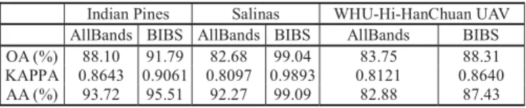
The band selection based on band importance is used to select spectral channels that are useful for classification and to alleviate the effects of noise bands. On the other hand, the band selection has a great impact on the classification accuracy of the CRFBS algorithm. For evaluation, the contribution of band selection for the CRFBS algorithm is measured in this subsection: we com-pare the classification results using all spectral bands (AllBands) and selected bands based on band importance (BIBS) for the three experimental datasets (Table IX).
The spectral-spatial classification method based on CRF mod-els the basic discriminative information of various semantic classes based on the used spectral bands by unary potentials. Accordingly, the selected spectral channels also affect the clas-sification results of the CRFBS algorithm. As can be observed from Table IX, the algorithm using the selected bands based on band importance can achieve a more than 3%, 10% and 4% improvement in OA for the Indian Pines, Salinas and WHU-Hi-HanChuan UAV datasets, respectively, compared with that achieved using all spectral bands. This demonstrates that the band selection can improve the spectral-spatial classification accuracies of CRF and play an important role for the CRFBS algorithm.
VI. CONCLUSION
In this study, a spectral-spatial classification algorithm based on CRF integrating band selection (CRFBS) has been developed and systematically tested for hyperspectral image with severe noise bands. On the one hand, the hyperspectral data can have very noisy bands, and may even have bands which feature solely zero values and do not contain any useful information. It has been shown that the proposed algorithm can automatically select the bands that are useful for classification to eliminate the effects of severe noise bands and reduce the need for high-quality image data. On the other hand, the CRFBS algorithm can integrate the spectral and spatial information by modeling the spatial interac-tions between pixels and combining the advantages of the RF and SVM algorithms to improve the classification performance. The experiments using three different hyperspectral datasets with
noise bands confirmed that the proposed algorithm can achieve an improvement in classification performance, compared with other state-of-the-art spectral-spatial classification methods. In the future, the accurate estimation of the class membership probabilities will be considered to model the unary potentials of the CRF model, considering the inaccuracy of the probability estimation of the SVM algorithm.
ACKNOWLEDGMENT
The authors would like to thank the editor, associate editor and anonymous reviewers for their helpful comments and sugges-tions and also like to thank M. Wang and X. Hu for their help with the comparison experiments. Ji Zhao gratefully acknowledges the support of K. C. Wong Education Foundation and German Academic Exchange Service.
REFERENCES
[1] C.-I. Chang, Hyperspectral Imaging: Techniques for Spectral Detection
and Classification. New York, NY, USA: Kluwer, 2003.
[2] R. Feng, L. Wang, and Y. Zhong, “Least angle regression-based con-strained sparse unmixing of hyperspectral remote sensing imagery,”
Re-mote Sens., vol. 10, 2018, Art. no. 1546.
[3] L. He, J. Li, C. Liu, and S. Li, “Recent advances on spectral–spatial hy-perspectral image classification: An overview and new guidelines,” IEEE
Trans. Geosci. Remote Sens., vol. 56, no. 3, pp. 1579–1597, Mar. 2018.
[4] M. J. Khan, H. S. Khan, A. Yousaf, K. Khurshid, and A. Abbas, “Modern trends in hyperspectral image analysis: A review,” IEEE Access, vol. 6, pp. 14118–14129, 2018.
[5] G. Hughes, “On the mean accuracy of statistical pattern recognizers,” IEEE
Trans. Inf. Theory, vol. 14, no. 1, pp. 55–63, Jan. 1968.
[6] W. Sun and Q. Du, “Hyperspectral band selection: A review,” IEEE Geosci.
Remote Sens. Mag., vol. 7, no. 2, pp. 118–139, Jun. 2019.
[7] M. Wang, J. Yu, L. Niu, and W. Sun, “Feature extraction for hyperspectral images using low-rank representation with neighborhood preserving reg-ularization,” IEEE Geosci. Remote Sens. Lett., vol. 14, no. 6, pp. 836–840, Jun. 2017.
[8] D. Hong, N. Yokoya, and X. X. Zhu, “Learning a robust local manifold representation for hyperspectral dimensionality reduction,” IEEE J. Sel.
Topics Appl. Earth Observ. Remote Sens., vol. 10, no. 6, pp. 2960–2975,
Jun. 2017.
[9] S. Jia, Z. Ji, Y. Qian, and L. Shen, “Unsupervised band selection for hyperspectral imagery classification without manual band removal,” IEEE
J. Sel. Topics Appl. Earth Observ. Remote Sens., vol. 5, no. 2, pp. 531–543,
Apr. 2012.
[10] W. Sun, L. Tian, Y. Xu, D. Zhang, and Q. Du, “Fast and robust self-representation method for hyperspectral band selection,” IEEE J. Sel.
Topics Appl. Earth Observ. Remote Sens., vol. 10, no. 11, pp. 5087–5098,
Nov. 2017.
[11] P. Su, D. Liu, X. Li, and Z. Liu, “A saliency-based band selection approach for hyperspectral imagery inspired by scale selection,” IEEE Geosci.
Remote Sens. Lett., vol. 15, no. 4, pp. 572–576, Apr. 2018.
[12] Q. Wang, J. Lin, and Y. Yuan, “Salient band selection for hyperspectral image classification via manifold ranking,” IEEE Trans. Neural Netw.
Learn. Syst., vol. 27, no. 6, pp. 1279–1289, Jun. 2016.
[13] M. Belgiu and L. Dr˘agu¸t, “Random forest in remote sensing: A review of applications and future directions,” ISPRS J. Photogrammetry Remote
Sens., vol. 114, pp. 24–31, Apr. 2016.
[14] G. Mountrakis, J. Im, and C. Ogole, “Support vector machines in remote sensing: A review,” ISPRS J. Photogrammetry Remote Sens., vol. 66, pp. 247–259, May 2011.
[15] C. Geiß, P. Aravena Pelizari, L. Blickensdörfer, and H. Taubenböck, “Virtual support vector machines with self-learning strategy for classifica-tion of multispectral remote sensing imagery,” ISPRS J. Photogrammetry
Remote Sens., vol. 151, pp. 42–58, May 2019.
[16] R. Khatami, G. Mountrakis, and S. V. Stehman, “A meta-analysis of remote sensing research on supervised pixel-based land-cover image classification processes: General guidelines for practitioners and future research,”
[17] J. Xia, J. Chanussot, P. Du, and X. He, “Spectral–spatial classification for hyperspectral data using rotation forests with local feature extraction and Markov random fields,” IEEE Trans. Geosci. Remote Sens., vol. 53, no. 5, pp. 2532–2546, May 2014.
[18] J. Xia, J. Chanussot, P. Du, and X. He, “Rotation-based support vector machine ensemble in classification of hyperspectral data with limited training samples,” IEEE Trans. Geosci. Remote Sens., vol. 54, no. 3, pp. 1519–1531, Mar. 2016.
[19] P. Duan, X. Kang, S. Li, and P. Ghamisi, “Noise-robust hyperspectral image classification via multi-scale total variation,” IEEE J. Sel. Topics Appl.
Earth Observ. Remote Sens., vol. 12, no. 6, pp. 1948–1962, Jun. 2019.
[20] M. Fauvel, Y. Tarabalka, J. A. Benediktsson, J. Chanussot, and J. C. Tilton, “Advances in spectral–spatial classification of hyperspectral images,”
Proc. IEEE, vol. 101, no. 3, pp. 652–675, Mar. 2013.
[21] L. Sun, C. Ma, Y. Chen, H. J. Shim, Z. Wu, and B. Jeon, “Adjacent superpixel-based multiscale spatial-spectral kernel for hyperspectral clas-sification,” IEEE J. Sel. Topics Appl. Earth Observ. Remote Sens., vol. 12, no. 6, pp. 1905–1919, Jun. 2019.
[22] T. Blaschke, “Object based image analysis for remote sensing,” ISPRS J.
Photogrammetry Remote Sens., vol. 65, pp. 2–16, Jan. 2010.
[23] H. Taubenböck, T. Esch, M. Wurm, A. Roth, and S. Dech, “Object-based feature extraction using high spatial resolution satellite data of urban areas,” J. Spatial Sci., vol. 55, pp. 117–132, 2010.
[24] C. Geiß, M. Klotz, A. Schmitt, and H. Taubenböck, “Object-based mor-phological profiles for classification of remote sensing imagery,” IEEE
Trans. Geosci. Remote Sens., vol. 54, no. 10, pp. 5952–5963, Oct. 2016.
[25] H. Luo, L. Wang, C. Wu, and L. Zhang, “An improved method for im-pervious surface mapping incorporating LiDAR data and high-resolution imagery at different acquisition times,” Remote Sens., vol. 10, 2018, Art. no. 1349.
[26] M. Baatz and A. Schäpe, “Multiresolution Segmentation: an optimization approach for high quality multi-scale image segmentation,” in Proc.
Ange-wandte Geographische Informations-Verarbeitung XII, Wichmann Verlag,
Karlsruhe, 2000, pp. 12–23.
[27] C. Geiß and H. Taubenböck, “Object-based postclassification relearn-ing,” IEEE Geosci. Remote Sens. Lett., vol. 12, no. 11, pp. 2336–2340, Nov. 2015.
[28] L. Zhang, L. Zhang, and B. Du, “Deep learning for remote sensing data: A technical tutorial on the state of the art,” IEEE Geosci. Remote Sens.
Mag., vol. 4, no. 2, pp. 22–40, Jun. 2016.
[29] N. Audebert, B. Le Saux, and S. Lefevre, “Deep learning for classification of hyperspectral data,” IEEE Geosci. Remote Sens. Mag., vol. 7, no. 2, pp. 159–173, Jun. 2019.
[30] S. Li, W. Song, L. Fang, Y. Chen, P. Ghamisi, and J. A. Benediktsson, “Deep learning for hyperspectral image classification: An overview,” IEEE Trans.
Geosci. Remote Sens., vol. 57, no. 9, pp. 6690–6709, Sep. 2019.
[31] X. Li, Z. Tang, W. Chen, and L. Wang, “Multimodal and multi-model deep fusion for fine classification of regional complex landscape areas using ZiYuan-3 imagery,” Remote Sens., vol. 11, 2019, Art. no. 2716. [32] X. Mei et al., “Spectral-spatial attention networks for hyperspectral image
classification,” Remote Sens., vol. 11, 2019, Art. no. 963.
[33] Z. Zhong, J. Li, Z. Luo, and M. Chapman, “Spectral–spatial residual network for hyperspectral image classification: A 3-D deep learning frame-work,” IEEE Trans. Geosci. Remote Sens., vol. 56, no. 2, pp. 847–858, Feb. 2018.
[34] Y. Zhong, J. Zhao, and L. Zhang, “A hybrid object-oriented conditional random field classification framework for high spatial resolution remote sensing imagery,” IEEE Trans. Geosci. Remote Sens., vol. 52, no. 11, pp. 7023–7037, Nov. 2014.
[35] P. Zhong and R. Wang, “Jointly learning the hybrid CRF and MLR model for simultaneous denoising and classification of hyperspectral imagery,”
IEEE Trans. Neural Netw. Learn. Syst., vol. 25, no. 7, pp. 1319–1334,
Jul. 2014.
[36] J. Zhao, Y. Zhong, and L. Zhang, “Detail-preserving smoothing classifier based on conditional random fields for high spatial resolution remote sensing imagery,” IEEE Trans. Geosci. Remote Sens., vol. 53, no. 5, pp. 2440–2452, May 2015.
[37] J. Li, J. M. Bioucas-Dias, and A. Plaza, “Spectral-spatial classification of hyperspectral data using loopy belief propagation and active learning,”
IEEE Trans. Geosci. Remote Sens., vol. 51, no. 2, pp. 844–856, Feb. 2013.
[38] J. Zhao et al., “Spectral-spatial classification of hyperspectral imagery with cooperative game,” ISPRS J. Photogrammetry Remote Sens., vol. 135, pp. 31–42, Jan. 2018.
[39] J. D. Lafferty, A. McCallum, and F. C. N. Pereira, “Conditional random fields: Probabilistic models for segmenting and labeling sequence data,” in Proc. 18th Int. Conf. Mach. Learn., 2001, pp. 282–289.
[40] J. Zhao, Y. Zhong, H. Shu, and L. Zhang, “High-resolution image classi-fication integrating spectral-spatial-location cues by conditional random fields,” IEEE Trans. Image Process., vol. 25, no. 9, pp. 4033–4045, Sep. 2016.
[41] Y. Boykov, O. Veksler, and R. Zabih, “Fast approximate energy mini-mization via graph cuts,” IEEE Trans. Pattern Anal. Mach. Intell., vol. 23, no. 11, pp. 1222–1239, Nov. 2001.
[42] J. Zhao, Y. Zhong, X. Hu, L. Wei, and L. Zhang, “A robust spectral-spatial approach to identifying heterogeneous crops using remote sensing imagery with high spectral and spatial resolutions,” Remote Sens. Environ., vol. 239, Mar. 2020, Art. no. 111605.
[43] L. Breiman, “Random forests,” Mach. Learn., vol. 45, pp. 5–32, 2001. [44] J. Xia, P. Ghamisi, N. Yokoya, and A. Iwasaki, “Random forest ensembles
and extended multiextinction profiles for hyperspectral image classifica-tion,” IEEE Trans. Geosci. Remote Sens., vol. 56, no. 1, pp. 202–216, Jan. 2018.
[45] K. Tan, H. Wang, L. Chen, Q. Du, P. Du, and C. Pan, “Estimation of the spatial distribution of heavy metal in agricultural soils using airborne hyperspectral imaging and random forest,” J. Hazardous Mater., vol. 382, 2020, Art. no. 120987.
[46] C.-C. Chang and C.-J. Lin, “LIBSVM: A library for support vector machines,” ACM T. Int. Syst. Technol., vol. 2, pp. 1–27, Apr. 2011. [47] Y. Zhong et al., “Mini-UAV-borne hyperspectral remote sensing: From
observation and processing to applications,” IEEE Geosci. Remote Sens.
Mag., vol. 6, no. 4, pp. 46–62, Dec. 2018.
[48] M. Wang, C. Wu, L. Wang, D. Xiang, and X. Huang, “A feature selection approach for hyperspectral image based on modified ant lion optimizer,”
Knowl.-Based Syst., vol. 168, pp. 39–48, 2019.
Ji Zhao received the Ph.D. degree in photogrammetry and remote sensing from the State Key Laboratory of Information Engineering in Surveying, Mapping, and Remote Sensing, Wuhan University, China, in 2017. He is now an Associate Professor at the School of Computer Science, China University of Geosciences, Wuhan. His major research interests include high resolution remote sensing image classification, scene analysis, remote sensing applications, and machine learning algorithms.
Suzheng Tian received the B.E. degree in computer science and technology from the School of Computer Science, China University of Geosciences, Wuhan, China, in 2019. She is currently pursuing the M.S. degree in the School of Computer Science, China University of Geosciences, Wuhan, China. Her major research interests include machine learning methods and nighttime lights.
Christian Geiß (Member, IEEE) received the M.Sc. degree in applied geoinformatics from the Paris Lo-dron University of Salzburg, Salzburg, Austria, in 2010, and the Ph.D. degree (Dr. rer. nat.) from the Humboldt University of Berlin, Berlin, Germany, in 2014. Since 2010, he has been with the German Re-mote Sensing Data Center (DFD), German Aerospace Center (DLR), Weßling, Germany. In 2017, he was also with the Cambridge University Centre for Risk in the Built Environment (CURBE), University of Cambridge, Cambridge, U.K., as a Visiting Scholar. His current research interests include the development of machine learning methods for the interpretation of earth observation data, multimodal remote sensing of the built environment, exposure and vulnerability assessment in the context of natural hazards, and techniques for automated damage assessment after natural disasters.
Lizhe Wang is the “ChuTian” Chair Professor at the School of Computer Science, China Univ. of Geo-sciences. He received the B.E. & M.E degrees from Tsinghua Univ. and the D.E. degree from Univ. Karl-sruhe (Magna Cum Laude), Germany. His research interests include remote sensing data processing, Dig-ital Earth, Big Data Computing. He is a Fellow of IET and BCS and Associate Editor of Remote Sensing, IJDE, etc. He is the recipient of Distinguished Young Scholars of NSFC, National Leading Talents of Sci-ence & Technology Innovation, 100-Talents Program of Chinese Academy of Sciences.
Yanfei Zhong (Senior Member, IEEE) received the B.S. degree in information engineering and the Ph.D. degree in photogrammetry and remote sensing from Wuhan University, China, in 2002 and 2007, respec-tively. Since 2010, He has been a Full professor with the State Key Laboratory of Information Engineering in Surveying, Mapping and Remote Sensing (LIES-MARS), Wuhan University, China. He organized the Intelligent Data Extraction, Analysis and Applica-tions of Remote Sensing (RSIDEA) research group. He has published more than 100 research papers in international journals, such as Remote Sensing of Environment, ISPRS Journal
of Photogrammetry and Remote Sensing, IEEE TRANSACTIONS ONGEOSCIENCE ANDREMOTESENSING. His research interests include hyperspectral remote sensing information processing, high-resolution remote sensing image under-standing, and geoscience interpretation for multisource remote sensing data and applications. Dr. Zhong is a Fellow of the Institution of Engineering and Technology (IET). He was a recipient of the 2016 Best Paper Theoretical Innovation Award from the International Society for Optics and Photonics (SPIE). He won the Second-Place Prize in 2013 IEEE GRSS Data Fusion Contest and the Single-view Semantic 3-D Challenge of the 2019 IEEE GRSS Data Fusion Contest, respectively. He is currently serving as an Associate Editor for the IEEE JOURNAL OFSELECTEDTOPICS INAPPLIEDEARTHOBSERVATIONS ANDREMOTESENSING, and the International Journal of Remote Sensing.
Hannes Taubenböck received the diploma in ge-ography from the Ludwig-Maximilians-Universität München, Munich, Germany, in 2004, and the Ph.D. degree (Dr. rer. nat.) in geography from the Julius-Maximilians-Universität Würzburg, Würzburg, Ger-many, in 2008. In 2005, he joined the German Re-mote Sensing Data Center (DFD), German Aerospace Center (DLR), Oberpfaffenhofen, Germany. After a postdoctoral research phase with the University of Würzburg (2007–2010), he returned in 2010 to DLR– DFD as a scientific employee. In 2013, he became the Head of the “City and Society” team. In 2019, he habilitated at the University of Würzburg in geography. His current research focuses on urban remote sensing topics, from the development of algorithms for information extraction to value adding to classification products for findings in urban geography.