Forecasting Exchange Rates Out-of-Sample with Panel Methods and Real-Time Data. Onur Ince * University of Houston

(1)

Forecasting Exchange Rates Out-of-Sample with Panel Methods and Real-Time Data†

Onur Ince* University of Houston

Abstract

This paper evaluates out-of-sample exchange rate forecasting with Purchasing Power Parity (PPP) and Taylor rule fundamentals for 9 OECD countries vis-à-vis the U.S. dollar over the period from 1973:Q1 to 2009:Q1 at short and long horizons. In contrast with previous work, which reports “forecasts” using revised data, I construct a quarterly real-time dataset that incorporates only the information available to market participants when the forecasts are made. Using bootstrapped out-of-sample test statistics, the exchange rate model with Taylor rule fundamentals performs better at the one-quarter horizon and panel specifications are not able to improve its performance. The PPP model, however, forecasts better at the 16-quarter horizon and its performance increases with the panel framework. The results are in accord with previous research on long-run PPP and estimation of Taylor rule models.

Keywords: Exchange Rate Forecasting, Taylor Rules, Real-Time Data, Out-of-Sample Test Statistics

JEL Classification: C23, C53, E32, E52, E58, F31, F47

†_{I thank David Papell for encouragement and guidance, and Chris Murray, Sebnem Kalemli-Ozcan, Nelson} Mark, Lutz Kilian, Tanya Molodtsova, James Morley, Claude Lopez, and Vania Stavrakeva for helpful comments and discussions.

* _{Department of Economics, University of Houston, Houston, TX 77204-5882. Tel: +1 (713) 743-3854.}

(2)

1 1. Introduction

Following the collapse of the Bretton-Woods system, the introduction of flexible exchange rate regimes attracted much attention to the area of international macroeconomics in an attempt to explain exchange rate behavior. Theoretical papers such as Dornbusch (1976), which extended the Mundell-Fleming model to incorporate rational expectations and sticky prices and introduced overshooting as an explanation for high exchange rate variability, and empirical work such as Frankel (1979), which found success in estimating empirical exchange rate models, inspired research in this field by pointing out the ability of macroeconomic models to explain exchange rate variability.

The seminal papers by Meese and Rogoff (1983a, 1983b) put an end to the atmosphere of optimism in exchange rate economics by concluding that empirical exchange rate models do not perform better than a random walk model out-of-sample. Their finding is still hard to overturn more than two decades later. Cheung, Chinn and Pascual (2005), for example, examine out-of-sample performance of the interest rate parity, monetary, productivity-based and behavioral exchange rate models, and suggest that none of the models consistently outperforms the random walk at any horizon.

Are empirical exchange rate models really as bad as we think? Recent studies have found evidence of exchange rate predictability using either panels or innovative modeling approaches. Engel, Mark, and West (2007) use panel specifications of the monetary, Purchasing Power Parity (PPP) and Taylor (1993) rule models, Rossi (2006) uses the monetary model in the presence of a structural break, Gourinchas and Rey (2007) use an external balance model, Molodtsova and Papell (2009) use a heterogeneous symmetric Taylor rule with smoothing, and Cerra and Saxena (2008) use a broad panel specification of the monetary model.

A common problem with the papers discussed above is their reliance on ex-post revised data for the forecasting analysis. Although it seems obvious that out-of-sample exchange rate forecasting should be evaluated using real-time data, which reflects information available to market participants, it is still very rare in the exchange rate literature. Almost all existing studies on exchange rate forecasting exploit revised data which contains future information, due to revisions and additions of new data, that is not available to either policymakers or market participants. Out-of-sample forecasting evaluations based on ex-post revised data yield misleading inferences about the exchange rate models and information problems of market agents are not accounted in the analysis.

(3)

2

The first paper to use real-time data to evaluate nominal exchange rate predictability is Faust, Rogers and Wright (2003). Examining the predictive ability of Mark’s (1995) monetary model using real-time data for Japan, Germany, Switzerland and Canada vis-à-vis the U.S, they report that the models consistently perform better using real-time data than fully revised data. However, none of the models perform better than the random walk model. More recently, Molodtsova, Nikolsko-Rzhevskyy, and Papell (2008, 2009) find evidence of predictability with Taylor rule fundamentals using real-time data for the Deutschmark/dollar and Euro/dollar exchange rates.

There are no studies on exchange rate forecasting with real-time data for a reasonably large number of countries over the post Bretton Woods period because of the limited availability of real-time data for countries other than the U.S. In this paper, I construct a quarterly real-real-time dataset that contains 9 OECD countries (Australia, Canada, France, Germany, Italy, Japan, Netherlands, Sweden, the United Kingdom) vis-à-vis the U.S. dollar over the period from 1973:Q1 to 2009:Q1 to evaluate both short and long-horizon out-of-sample forecasting performance of the linear exchange models using PPP and Taylor rule fundamentals. I construct real-time prices and inflation from the International Financial Statistics (IFS) country pages using the consumer price index (CPI), and estimate real-time output gaps with the industrial production index.

A problem associated with recent papers presenting evidence of exchange rate predictability is that these studies employ a test developed by Clark and West (2006) (henceforth, CW test). They propose an adjustment to the Diebold and Mariano (1995) and West (1996) (henceforth, DMW test) statistic that corrects for size distortions. If two models are non-nested, the DMW test is appropriate to compare the mean square forecast errors (MSFE’s). Applying DMW tests to compare the MSFE’s of two nested models, however, leads to non-normal test statistics, and using standard normal critical values usually results in very poorly sized tests with far too few rejections of the null. This is a problem for out-of-sample exchange rate forecasting because, since the null is a random walk, all tests with structural models are nested. While the CW adjustment produces a test with correct size, Rogoff and Stavrakeva (2008) argue that it cannot evaluate forecasting performance because it does not test the null hypothesis of equal MSFE’s of the random walk and the structural model. In order to satisfy the conditions for a “good” exchange rate forecasting model, empirical studies need to present evidence that the exchange rate model has MSFE that is significantly smaller than that of the random walk model, which cannot be done solely with CW test in the case of

(4)

3

forecasting bias.1_{They advocate the use of DMW tests with bootstrapped critical values to produce} correctly sized tests.

Engel, Mark and West (2007) find that panel error-correction exchange rate models with PPP fundamentals are able to produce large improvements in out-of-sample forecasting at longer horizons.2_{Because they use ex-post revised data, the exchange rate models in their study contain} future information that was not available to market participants. “Forecasting” exercises involving future news in the information set of the linear model cannot be evaluated as an out-of-sample forecasting exercise. Forecasts with real-time data, however, do not contain any unrealized future information in the information set of the linear model, and thus are a true out-of-sample forecast.

Molodtsova and Papell (2009) find evidence of out-of-sample predictability with the Taylor model at short horizon using single-equation estimation. Although they use ex-post revised data to calculate inflation, they estimate output gaps with quasi-real-time data in order to capture the information available to central banks as closely as possible. Quasi-real-time data is constructed with ex-post revised data, but the trends do not contain future observations and the data points are used with a lag for estimation. While quasi-real-time data does not contain future observations, it captures revisions which are not available to market participants. Therefore, forecasting exercises with quasi-real time data are also not true out-of-sample forecasts.

This paper evaluates out-of-sample forecasting with PPP and Taylor Rule fundamentals using my newly constructed real-time dataset for 9 OECD countries vis-à-vis the U.S. dollar with single-equation and panel error-correction frameworks based on bootstrapped DMW and CW test statistics.3_{The out-of-sample forecast results with PPP fundamentals confirm the findings in Engel,} Mark and West (2007) that the predictability of the PPP model increases with the panel specification and the PPP model has higher predictive power at long horizons. Evidence of long-term predictability with the PPP model is found for 6 out of 9 countries against the driftless random walk and for all the countries against the random walk with drift with panel framework. The exchange rate model with PPP fundamentals using panel data outperforms the driftless random walk for 5 out

1_{Rogoff and Stavrakeva (2008) consider the scale bias where the observed value is over- or under predicted} by a certain percent.

2_{Engel, Mark and West (2007) use monetary and Taylor Rule models as well. However, the out-of-sample} predictability of the PPP model dominates the other two models at longer horizons.

3_{I would like to evaluate the out-of-sample forecasting ability of the monetary model. However, it is not} possible to find coherent series of real-time money supply for all the countries.

(5)

4

of 9 countries and the random walk with drift for all the countries in the sample at the 16-quarter horizon.

The predictability of Taylor fundamentals, in contrast, is greatest with the single-equation specification, and the Taylor rule model has higher forecasting power at a short horizon as indicated in Molodtsova and Papell (2009). Evidence of short-term predictability with Taylor rule model is found for 1 out of 9 countries against the driftless random walk and for 4 out of 9 countries against the random walk with drift with single-equation estimation. The exchange rate model with Taylor rule fundamentals using a single-equation framework outperforms the driftless random walk for 1 out of 9 countries and the random walk with drift for 5 out of 9 countries at the one-quarter horizon.

The results are in accord with previous research on PPP and estimation of Taylor rule models. The PPP model works best with the panel specification at the 16-quarter horizon. Research on PPP shows no evidence at short-run PPP, and Papell (1997) finds considerably more support for long-run PPP with panel methods than with univariate tests. Panel models exploit the information contained in the high correlation between nominal and real exchange rates for the countries in our sample. The Taylor rule model performs better with single-equation estimation at the one-quarter horizon. Monetary policy rules implemented by central banks since the early-to-mid 1980s set interest rates for relatively short periods and are different from each other. Clarida, Gali and Gertler (1998) provide empirical evidence of how interest rate reaction functions differ among OECD countries. Gerdesmeier, Mongelli and Roffia (2007) compare the monetary policies implemented by the Eurosystem, the Fed and the Bank of Japan, and also find differences. Imposing identical monetary rules across all countries in a panel structure does not produce successful out-of-sample exchange rate forecasts, thus estimating the Taylor rule model with a single-equation framework performs better.

2. Data

The real-time quarterly data used in this study covers the post-Bretton Woods period from 1973:Q1 to 2009:Q1 for 10 OECD countries: Australia, Canada, France, Germany, Italy, Japan, Netherlands, Sweden, the United Kingdom, and the United States. The dataset is constructed from the country tables of IMF's International Financial Statistics (IFS) books, regularly published on a monthly basis since 1948. Seasonally adjusted industrial production index (IFS line 66c) is used as a

(6)

5

measure of countries’ income, since quarterly GDP data are not consistently published and not available for some countries for much of the time span. The price level in the economy is measured by the consumer price index (CPI) (IFS line 64) and seasonally adjusted by applying a one-sided moving average of the current observation and 3-lagged values. The inflation rate is the annual inflation rate calculated using the CPI over the previous 4 quarters. Nominal exchange rates are taken from the IFS CD-ROM (IFS line ae) defined as the end-of-period U.S. dollar price of a unit of foreign currency. Exchange rates for the Euro area after 1998 are normalized by fixing foreign currency per dollar to the Euro/Dollar rate as in Engel, Mark and West (2007).

The real-time data has the usual triangular format with vintage dates on the horizontal axis and calendar dates for each observation on the vertical axis. The series of real-time inflation and output gaps are constructed from the diagonal elements of the real-time data matrix and contain only the latest available observations at each period.For each country, this data represents a vector of quarterly observations from 1973:Q1 to 2009:Q1, thus resulting in 145 observations.

The output gap is calculated as the percentage deviation of actual output from a Hodrick-Prescott (1997) (HP) trend.4_{The industrial production index series in each data vintage that is used} to estimate the output gap goes back to 1958:Q1 for all countries. For the first data point, the trend is calculated using the data for 1958:Q1-1973:Q1, for the second data point, it is calculated using the data for 1958:Q1-1973:Q2, and so on. As with any method that uses a one-sided filter, the estimations might be subject to end-of-sample uncertainty which is exacerbated with real-time data, consisting of the last observations in each data vintage. To take into account the end-of-sample uncertainty in output gap estimation using real-time data, I use Watson’s (2007) correction and forecast the industrial production series 12 quarters ahead before calculating the trend.5

3. Methodology

The econometric analysis in this study is based on panel estimation of the predictive regression,

𝑠𝑖𝑡+𝑘 − 𝑠𝑖𝑡 = 𝛽𝑘𝑧𝑖𝑡 + 𝜀𝑖𝑡+𝑘 (1)

4_{The smoothness parameter for HP filter is 1600 for quarterly data.}

5_{While Watson (2007) also suggests to backcast the series, the series in each data vintage extends through} 1958:Q1, which is long enough to remove the distortions in the beginning of the sample created by a one-sided filter.

(7)

6

where zit = fit − sit and 𝜀𝑖𝑡 = 𝜁𝑖 + 𝜃𝑡 + 𝘶𝑖𝑡.6 In the predictive regression, sit denotes the natural log of the nominal exchange rate, measured as the domestic price of U.S. dollar (which serves as base currency) for country i at time t. The deviation of the exchange rate from its equilibrium value is denoted by z and f stands for the fundamental in the exchange rate model that is determined either by PPP or Taylor rule. The forecast horizon 𝑘, takes the value of 1 for short-horizon and 16 for long-horizon regressions. The regression error,εit, has unobserved components, where ζi is the

individual specific effect, 𝜃_𝑡 is the time-specific effect, and 𝘶_𝑖𝑡 is the residual idiosyncratic error. 3.1 PPP Fundamentals

Numerous studies that test for unit roots in real exchange rates using panels of industrialized countries have found strong rejections in the post-1973 period. The strong rejections of unit roots encourage testing the forecasting power of exchange rate models with PPP fundamentals. Recently, Engel, Mark and West (2007) have shown that PPP fundamentals forecast well at long horizons. Rogoff and Stavrakeva (2008) also conclude that PPP specification performs the best out of all the specifications they try.7

Under PPP fundamentals,

𝑓𝑖𝑡 = 𝑝0𝑡 − 𝑝𝑖𝑡 (2)

where 𝑝_0𝑡 is the log of price level of U.S. which serves as base country and 𝑝_𝑖𝑡 is the log of price level of country i. I use the real-time CPI as a measure of the national price level. Substituting PPP fundamentals (2) into (1), I use the resultant equation for forecasting.

3.2 Taylor Rule Fundamentals

When central banks set the interest rate according to the Taylor rule, the linkage between the exchange rate and a set of fundamentals can be examined. According to Taylor (1993), central banks set the monetary policy as:

𝑖_𝑡∗ _{= 𝜋}

𝑡 + ф(𝜋𝑡 − 𝜋∗) + 𝛾𝑦𝑡𝑔 + 𝑟∗ (3)

where 𝑖𝑡∗ is the target for the short-term nominal interest rate, 𝜋𝑡 is the inflation rate, 𝜋∗is the target

level of inflation, 𝑦_𝑡𝑔is the output gap, or percent deviation of actual output from an estimate of its potential level, and 𝑟∗_{is the equilibrium level of the real interest rate. It is assumed that the target for}

6_{For single-equation framework, time-specific effect is zero.}

7_{Rogoff and Stavrakeva (2008) compare the forecasting power of the monetary model, the Taylor rule model} and a structural model based on the Backus-Smith optimal risk sharing condition.

(8)

7

the short-term nominal interest rate is achieved within the period, so that there is no distinction between the actual and target nominal interest rate.

The parameters 𝜋∗_and_𝑟∗_{in equation (3) can be combined into one constant term}_{𝜇 =} 𝑟∗_{− ф𝜋}∗_{and we have:}

𝑖_𝑡∗ _{= 𝜇 + 𝜆𝜋}

𝑡 + 𝛾𝑦𝑡𝑔 (4)

where 𝜆 = 1 + ф. If the central bank sets the target the level of exchange rate to make PPP hold, equation (4) becomes:

𝑖_𝑡∗ _{= 𝜇 + 𝜆𝜋}

𝑡+ 𝛾𝑦𝑡𝑔 + 𝛿𝑞𝑡 (5)

where 𝑞_𝑡 is the real exchange rate. The central bank increases (decreases) the nominal interest rates if the exchange rate depreciates (appreciates) from its equilibrium value under PPP assumption in the Taylor rule. Allowing interest rates to achieve its target level within the period:

𝑖_𝑡 = 𝜇 + 𝜆𝜋_𝑡 + 𝛾𝑦_𝑡𝑔+ 𝛿𝑞_𝑡 (6) and 𝑖_𝑡 is the nominal interest rate. Subtracting the Taylor rule equation for the foreign country from that for the base country, the U.S. (denoted by “0”), equation (6) becomes:

𝑖_0𝑡 − 𝑖_𝑖𝑡 = 𝜆 𝜋_0𝑡 − 𝜋_𝑖𝑡 + 𝛾 𝑦_0𝑡𝑔 − 𝑦_𝑖𝑡𝑔 + 𝛿 𝑠_𝑖𝑡 + 𝑝_𝑖𝑡 − 𝑝_0𝑡 (7) Imposing the uncovered interest rate parity condition 𝐸𝑡𝑠𝑖𝑡+1 = 𝑖𝑖𝑡 − 𝑖0𝑡 + 𝑠𝑖𝑡, the expected change

in nominal exchange rates is equal to the interest differential:

𝐸_𝑡𝑠_𝑖𝑡+1 = 𝜆 𝜋_0𝑡 − 𝜋_𝑖𝑡 + 𝛾 𝑦_0𝑡𝑔 − 𝑦_𝑖𝑡𝑔 + 𝛿 𝑠_𝑖𝑡 + 𝑝_𝑖𝑡 − 𝑝_0𝑡 + 𝑠_𝑖𝑡 (8) Molodtsova and Papell (2009) refer to specification (8) as homogenous asymmetric Taylor rule with no smoothing. They estimate the parameters 𝜆, 𝛾, and 𝛿 in equation (8) in a rolling regression framework. However, I follow the approach developed by Engel, Mark and West (2007). Rather than estimating the coefficients, they posit a Taylor rule such that 𝜆=1.5, 𝛾=0.1 and 𝛿=0.1. The Taylor rule fundamentals to be used in forecasting equation (1) become:

𝑓_𝑖𝑡 = 1.5 𝜋_0𝑡 − 𝜋_𝑖𝑡 + 0.1 𝑦_0𝑡𝑔 − 𝑦_𝑖𝑡𝑔 + 0.1 𝑠_𝑖𝑡 + 𝑝_𝑖𝑡 − 𝑝_0𝑡 + 𝑠_𝑖𝑡 (9) It is well known in the literature that the uncovered interest rate parity condition does not hold in the short run. With an error correction specification, the exchange rate forecasting model, 𝐸_𝑡𝑠_{𝑖𝑡+𝑘}− 𝑠_𝑖𝑡 = 𝛽_𝑘 𝑓_𝑖𝑡 − 𝑠_𝑖𝑡 , is used to generate out-of-sample forecasts both at the short-horizon (where k=1) and the long-short-horizon (where k=16).

(9)

8 4. Out-of-Sample Forecasting

4.1 Estimation

To produce out-of-sample forecasts, the sample has to be split into two components, in-sample and out-of-in-sample. The in-in-sample component is used to estimate the parameters in equation (1) within both the single-equation and the panel frameworks. The remaining out-of-sample component is usedfor out-of-sample forecasting.

Following Mark and Sul (2001) and Engel, Mark and West (2007), I estimate the predictive regression by least squares dummy variable (LSDV) using observations through the end of the in-sample component, 1982:Q4. For k=1(k=16), the predictive regression is used to forecast 1-step-ahead (16-step-1-step-ahead) exchange rate returns in 1983:Q1 (1986:Q4). Then, the in-sample component is updated recursively by extending the sample up to 1983:Q1 and equation (1) is re-estimated again. For k=1 (k=16), the predictive regression is used to forecast 1-step-ahead (16-step-ahead) exchange rate returns in 1983:Q2 (1987:Q1), and the loop continues until the last observation. At the end, 105 forecasts for k=1 and 90 overlapping forecasts for k=16 are derived with both PPP and Taylor rule fundamentals.

One crucial point for multi-period ahead forecasts in the panel framework is that the time effect needs to be forecasted. For k-period ahead forecasts, the time effect in period t+k is calculated by taking the recursive mean of the time effect until period t, such as 𝜃 _𝑡+𝑘 = 1_𝑡 𝑡 𝜃 _𝑗

𝑗 =1 .

4.2 Comparisons of Forecasts Based on MSFE

To compare the out-of-sample forecasting ability of the two nested models, this study focuses on the minimum mean-squared forecast error (MSFE) approach, which became dominant in the literature after Meese and Rogoff (1983a, 1983b). Forecasts of linear and random walk models are calculated as:

Linear Model: 𝛥𝑠 𝑖𝑡+𝑘 = 𝜁 𝑖+ 1_𝑡 𝑡𝑗 =1𝜃 𝑗 + 𝛽 𝑧𝑖𝑡

Driftless Random Walk: 𝛥𝑠 _{𝑖𝑡+𝑘} = 0 (10) Random Walk with Drift: 𝛥𝑠 _{𝑖𝑡+𝑘} = 𝛼 _𝑖𝑡

(10)

9

where 𝛼 is the estimated drift term.8_{Taking the difference between actual and predicted values of} exchange rates gives the forecast error. The MSFE approach selects a model which has significantly smaller MSFE than the random walk with or without the drift.

4.3 Out-of-Sample Test Statistics

To measure the relative forecast accuracy of the linear model against the driftless random walk and the random walk with drift, I use two alternative test statistics: the Diebold-Mariano and West (DMW) and the Clark-West (CW) statistics.

4.3.1 The Diebold-Mariano and West (DMW) Test

Suppose that a martingale difference process and a linear model are given as: Model 1: yt et Model 2: yt  Xtet ' _where 0 ) ( 1   t t e E

where the dependent variable is the change in the exchange rate. Under the null hypothesis, population parameter  0 and exchange rate follows a random walk. For simplicity let us concentrate on one-step-ahead forecasting. Assume that sample size is T+1; the first R observations are used for estimation and P is equal to the number of forecasts. So we have, T+1=R+P, where

T+1=145, R=40 and P=105 for one-step-ahead forecasting. Information prior to 𝑡 is used to forecast for period t=R, R+1, R+2, …, T. The first forecast is for the period R+1 and the final forecast is for the period T+1.

The estimated forecasts for the random walk and the structural model are 0 andXt t '

1 and



t

 is the regression estimate of t . After estimating the forecasts, the respective forecast errors for

the models are eˆ1,t1 yt1 and eˆ2,t1  yt1Xt1ˆt. Thus, the sample MSFE’s of the two models

become: 



     T P T t t y P 1 2 1 1 2 1 ˆ  and



      _ _  T P T t t t t X y P 1 2 1 1 1 2 2 ( ˆ ) ˆ   (11)

8_{The recursive mean of the time effect in parenthesis for the linear model is removed in the single-equation} case.

(11)

10

Diebold and Mariano (1995) and West (1996) construct a t-type statistics which is assumed to be asymptotically normal and the population MSFE’s are equal under the null. Defining the following equations, 2 , 2 2 , 1 ˆ ˆ ˆ t t t e e f  



     _ _  T P T t t f P f 1 2 2 2 1 1 1 ˆ _ˆ _ˆ ₍₁₂₎



     _  T P T t t f f P V 1 2 1 1 ) ˆ ( ˆ

The DMW test statistic is

P V f DMW ˆ 1   (13) The asymptotic DMW test works fine with non-nested models. However, the size properties of the asymptotic DMW test have been widely criticized for nested models. Clark and McCracken (2001, 2005) and McCracken (2007) show that the limiting distribution of the DMW test for nested models under the true null is not standard normal. Undersized DMW tests cause too few rejections of the null and may miss the statistical significance of the linear exchange rate model against the random walk.

4.3.2 The Clark- West (CW) Test

Clark and West (2006, 2007) show that the sample difference between the MSFE’s of two nested models in DMW test is biased downward from zero in favor of the random walk.



                           _ _ _ _ _ _ _ _   T P T t t t T P T t t t t T P T t t t t T P T t t T P T t t P y P y X P y X P X f P 1 2 1 1 1 1 1 1 1 2 1 1 1 1 2 1 1 1 1 1 2 2 2 1 ˆ ˆ ( ˆ ) 2 ˆ ( ˆ ) ˆ      (14)

Under the null hypothesis, the exchange rate follows a random walk, such that e1,t1 e2,t1  yt1.

(12)

11

equation (14) is equal to zero.9_{Clark and West (2006, 2007) show that} _        T P T t t t X P 1 0 2 ) ˆ 1 ( 1 _

because estimating the parameters of the alternative model under the true null (which are zero) brings noise into the forecasting process. Clark and West (2006) recommend an adjusted DMW statistic that adjusts for the negative bias in the difference between the two MSFE. Defining the adjustments as follows,



_ˆ ₎2



1 ( 2 1 , 2 ˆ 2 1 , 1 ˆ 1 ˆ t t X t e t e ADJ t f _  _  _  _ 



                _ _    T P T t T P T t t t ADJ t ADJ X P f P f 1 1 2 1 1 2 2 2 1 1 1 ) ˆ ( ˆ ˆ ˆ _ _ _ ₍₁₅₎



     _  T P T t ADJ ADJ t f f P V 1 2 1 1 ) ˆ ( ˆ

the CW test statistic is

ADJ ADJ V P f CW ˆ 1   (16) The CW test has become one the most popular out-of-sample test statistic in the exchange rate literature. However, Rogoff and Stavrakeva (2008) show that the CW test cannot always be interpreted as a minimum MSFE test as the DMW test. Their study presents a proof that in the presence of forecast bias, the null hypothesis of the CW and the DMW tests are not necessarily the same.10_{If one can reject the null of CW test, the true nature of exchange rate does not follow a} random walk. Nevertheless, even if the true model follows some other model rather than a random walk, one can still apply the DMW statistics to test whether the random walk and the structural model have equal MSFEs.

9 _       T P T t t t X t y 1 ˆ 1

1  is zero, because the equality of e1,t1e2,t1 under null hypothesis suggests that ) ˆ 1 1 , 2 ( ) ˆ 1 1 , 1 ( ) ˆ 1 1 (y_t X_t _t E e _t X_t _t Ee _t X_t _t

E _ _   _ _   _ _  . Since E(e₂_,_t_₁X_t_₁)0 by assumption, we have 0 ) ˆ 1 1 , 2 ( ) ˆ ( ) 1 1 , 2 (e _t_ X_t_ E _t E e _t_ X_t_ _t  E   .

(13)

12 4.4 Bootstrapping Out-of-Sample Test Statistics

Size distortions of the DMW test in small samples can be reduced by bootstrapping the finite sample distribution of the test statistics. Kilian (1999) state that unlike asymptotic critical values, correctly specified (maintaining the cointegration between the exchange rate and fundamentals under the null hypothesis) bootstrap critical values adapt for the increase in the dispersion of the finite-sample distribution by itself. Kilian (1999) also suggest that the bootstrap is appropriate for multi-period ahead forecasts. Based on simulation evidence, Li and Maddala (1997) and Li (2000) also indicate bootstrapped tests have smaller size distortions and higher test power than asymptotic tests in cointegrating systems. Howbeit, Berkowitz and Kilian (2000) emphasize the importance of bootstrapping type implemented to preserve cointegrating relationships in the data. They argue that cointegration appears to be a parametric notion and parametric bootstraps are more accurate than non-parametric ones.

Mark and Sul (2001) and Rogoff and Stavrakeva (2008) apply bootstrapped out-of-sample tests to detect forecasting ability of linear exchange rate models against random walk in a panel framework. The bootstrap methods are similar in both studies. Mark and Sul (2001) implement parametric bootstrap and estimate error correction equations with seemingly unrelated regressions (SURs); however, Rogoff and Stavrakeva (2008) use semi-parametric bootstrap and estimate error correction equations with country specific OLS regressions.

Having insignificant bootstrapped DMW test statistics in certain cases, as opposed to highly significant asymptotic CW test, Rogoff and Stavrakeva (2008) criticize the asymptotic CW test to be oversized and has less power than the bootstrapped DMW test in the presence of forecast bias.11 Oversized asymptotic CW test would cause too many rejections of the null hypothesis that exchange rate does not follow a random walk. It may detect spurious statistical significance and favor the alternative, structural exchange rate model. In this paper, I evaluate the out-of-sample forecasting ability of exchange rate fundamentals based on the bootstrapped DMW test, and the out-of-sample predictability of exchange rate fundamentals based on the bootstrapped CW test.

Rogoff and Stavrakeva’s (2008) method of bootstrap (which imposes cointegration restriction between the exchange rate and the fundamentals) for each country is used in this study as follows:

11_{In the technical appendix of Clark and West (2007), the unadjusted power of the bootstrapped DMW test} is higher than that of the asymptotic CW test for recursive regressions with one-step-ahead forecasts.

(14)

13 st t₍₁₈₎                d j l j t u j t z j j t s j t z t t z 1 1 1    

wheres_tis the nominal exchange rate and t

z _{is the deviation of exchange rate from fundamental as} defined in equation (1). s_t s_t s_t__k and z_t  z_t z_t__k where k is the forecast horizon,  is a constant and t is a trend. To control for autocorrelation in the error correction equation (ECE) lags of s_tand z_tare included. Akaike’s information criterion is used for each country to determine the optimum number of dand l and to figure out whether to include a constant or a trend or both in the ECE. The sum of coefficients on lags of z_tis restricted to 1. s_t andz_t_are simulated recursively after re-sampling the estimated residuals (_t and u_t ). To reduce the bias caused by the initial values of the recursion, the first 100 observations are thrown away and a new sample is created. Applying the estimation procedure again, test statistics are calculated with the pseudo-data. This process is repeated 1000 times and semi-parametric bootstrap distribution is derived. Since the tests considered are one-sided tests, the p-values of DMW and CW tests are the percentage of the bootstrapped distribution above the estimated test statistic using the realized data. 5. Empirical Results

This section summarizes one- and 16-quarter-ahead out-of-sample predictive and forecasting performance of the linear exchange rate model with PPP and Taylor Rule fundamentals to that of the random walk model with and without drift using a newly constructed real-time dataset. The tables report the MSFE ratio, the ratio of MSFE of the structural model to that of the random walk, and the DMW and CW test statistics with their respective bootstrapped p-values.

It is important to interpret the results of the DMW and CW tests correctly. The DMW test is a minimum MSFE test that compares the MSFE of the linear exchange rate model to that of the random walk. A significant DMW test statistic implies that the linear exchange rate model produces a lower MSFE than the random walk. The forecasting ability of the structural model is higher and the structural model outperforms the random walk out-of-sample. On the other hand, the CW test is a test of predictability where a significant CW test statistic indicates that the coefficients in the linear exchange rate model are jointly different from zero, and the random walk null can be rejected in

(15)

14

favor of the linear model alternative. We call rejections of the equal MSFE null hypothesis with the DMW test evidence of forecasting ability, and rejections of the random walk null hypothesis with the CW test evidence of predictability.

5.1 PPP Fundamentals

One-quarter-ahead single-equation forecast results with the PPP model are presented in Table 1. No evidence of either out-of-sample predictability or forecasting ability is found for the PPP model against the driftless random walk for any exchange rate. The out-of-sample forecasting performance of the PPP model improves against the random walk with drift. Short-term predictability is found for Canada and Sweden, and the PPP model outperforms the random walk with drift for 4 countries (Canada, Germany, Japan, and Netherlands) at the one-quarter horizon.

Panel one-quarter-ahead forecasts using PPP fundamentals in Table 2 are only slightly better than single-equation forecasts in Table 1. The exchange rate model with PPP fundamentals using panel data significantly outperforms the driftless random walk only for Japan. The evidence of predictability and forecasting ability of the PPP model with panel estimation, just like in the single-equation case, increases against the random walk with drift at one-quarter horizon. Short-term predictability is found for 5 out of 9 countries (Australia, Canada, Germany, Japan, and Sweden) and the PPP model forecasts better than the random walk with drift for Australia and Sweden.

The low predictive and forecasting power at the one-quarter horizon of the PPP model using panel and single-equation estimations is not surprising. Existing studies concerning the half-life of PPP, the expected number of years for a PPP deviation to decay by 50%, find half-lives of around 2.5 years.12_{Accounting for the slow adjustment of real exchange rates in advanced} economies, one would expect the predictability and forecasting ability of PPP model to be low at short horizons.13

Sixteen-quarter-ahead out-of-sample forecasts of the PPP model with single-equation estimation are presented in Table 3. The evidence of long-term predictability is stronger compared to one-quarter-ahead forecasts using the single-equation framework with rejections of the random walk null found for 4 countries (France, Germany, Netherlands, and Sweden). The PPP model,

12_{See Wu (1996), Papell (1997, 2002), Murray and Papell (2002), Choi, Mark and Sul (2006) for details} concerning the half-lives of PPP deviations.

13_{The correlations between real and nominal exchange rates are very high for almost all the countries in our} sample.

(16)

15

however, does not significantly forecast better than the driftless random walk for any exchange rate. More evidence of long-term predictability is found against the random walk with drift. Out-of-sample exchange rate predictability is found for 7 out of 9 countries (Australia, Canada, France, Germany, Japan, Netherlands, and Sweden) and the PPP model forecasts better than the random walk with drift for Australia, Canada and Netherlands. The out-of-sample predictability and forecasting ability of the PPP model with a single-equation framework is clearly improved at the l6-quarter horizon compared to one-l6-quarter horizon.

The PPP model performs best with the panel specification at the 16-quarter horizon. As reported in Table 4, the evidence of predictability is found for 6 out of 9 countries (Canada, France, Germany, Japan, Netherlands, and Sweden), and the PPP model forecasts better than the driftless random walk for 5 countries (Canada, Germany, Japan, Netherlands and Sweden). Panel forecasts at long horizon are even more striking against the random walk with drift. Out-of-sample predictability and forecasting ability is found for all the countries in the sample, as the exchange rate model with PPP fundamentals significantly outperforms the random walk with drift for each country using panel data. Because the commonality of high correlation between real and nominal exchange rates for the countries in the sample can be captured with the panel specification, panel estimation becomes more efficient and the predictability and forecasting ability of the panel exchange rate model with PPP fundamentals is much higher than the single-equation framework.

5.2 Taylor Rule Fundamentals

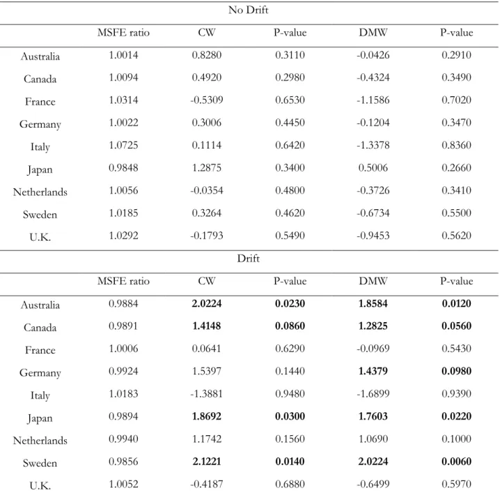
Following Engel, Mark, and West (2007), predictive regressions using Taylor rule model are estimated where the coefficients on inflation, output gap, and real exchange rate are fixed at certain values. One-quarter-ahead single-equation forecasts with Taylor rule are reported in Table 5. Evidence of short-term predictability and forecasting ability is found only for Japan. The exchange rate model with Taylor fundamentals works much better against the random walk with drift. Evidence of out-of-sample predictability and forecasting ability is found for 4 out of 9 countries (Australia, Canada, Japan, and Sweden), and evidence of forecasting ability is found for Netherlands. Comparing Tables 5 and 6, evaluating the performance of Taylor rules in a panel framework does not improve the results, as incorporating different monetary policies operated by central banks

(17)

16

in a panel framework does not help to forecast exchange rates out-of-sample.14_{One-quarter ahead} forecasting results for the Taylor rule model with a panel framework are reported in Table 6. No evidence of out-of-sample predictability or forecasting ability against the driftless random walk, as neither the equal MSFE nor the random walk null hypotheses can be rejected for any exchange rate. The results are stronger against the random walk with drift. Evidence of predictability is found for 4 out of 9 countries (Australia, Canada, Japan, and Sweden), and the Taylor rule model using panel estimation forecasts better than the random walk with drift for 5 out of 9 countries (Australia, Canada, Germany, Japan, and Sweden).

Table 7 presents 16-quarter-ahead single-equation forecasts using the Taylor rule model. There is no evidence of forecasting ability, and evidence of long-term predictability is found only for Germany against the driftless random walk. The single equation forecasts with the Taylor rule model perform better against the random walk with drift. Evidence of long-term predictability is found for Netherlands and Sweden, and evidence of forecasting ability for 5 out 9 countries (Australia, Canada, Japan, Netherlands, and Sweden).

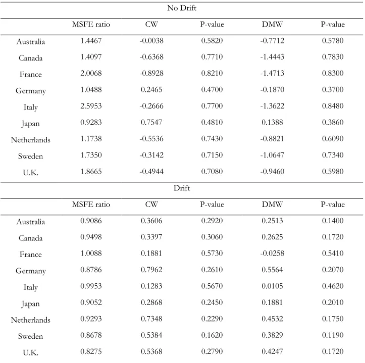
Panel forecasts with the Taylor rule model at the 16-quarter horizon perform poorly. As reported in Table 8, no evidence of either long-term predictability or forecasting ability is found against the random walk, with or without drift, for any of the countries in the sample. These results are in accord with previous work using revised or quasi-real-time data. Molodtsova and Papell (2009) report that the evidence of short term predictability disappears at longer horizons with a single equation Taylor rule model, and Engel, Mark and West (2007) do not find more evidence of predictability with panel models.

6. Conclusions

The vast majority of empirical studies on exchange rate forecasting over the post-Bretton Woods period use ex-post revised data. Since this data contains future information that is not available to policymakers and market participants at the time forecasts are made, it cannot be used to evaluate predictability and forecasting ability of exchange rate models out-of-sample. The use of

14_{See Clarida, Gali and Gertler (1998) and Gerdesmeier, Mongelli and Roffia (2007) for comparisons of} interest rate reaction functions among countries.

(18)

17

real-time data overcomes this problem and mimics the information set of market agents as closely as possible.

The purpose of this paper is to investigate how real-time data affects out-of-sample exchange rate forecasts of PPP and the Taylor rule models at short and long horizons with single-equation and panel frameworks. Our results show that panel estimation increases the predictability and the forecasting ability of the PPP model relative to single-equation estimation. The high correlation between real and nominal exchange rates of the countries in our sample is better captured by the panel specification and estimating the predictive regression with panel data increases the predictive and forecasting power of the PPP model. At the 16-quarter horizon, evidence of predictability is found with panel estimation for 6 out of 9 countries against the driftless random walk and for all of the countries against the random walk with drift based on the bootstrapped CW test. The PPP model using panel data outperforms the driftless random walk for 5 out of 9 countries and outperforms the random walk with drift for all the countries in the sample based on the bootstrapped DMW test. One-quarter-ahead forecasts of the exchange rate model with PPP fundamentals are weaker than long-horizon forecasts. The good predictability and forecasting ability of the PPP model at longer-horizons is in accord with estimated half-lives of PPP deviations of around 2.5 years. The predictability and the forecasting ability of the PPP model at longer horizons with panel estimation confirms the findings in Engel, Mark and West (2007).

In contrast, out-of-sample forecasting with panel models are unable to improve forecasts compared with single-equation estimation for the exchange rate model with Taylor rule fundamentals. As shown in Clarida, Gali and Gertler (1998), interest rate functions are different among the OECD countries, and so the assumption of identical monetary policy rules for all the central banks in panels is not very realistic. With both single-equation and panel error correction models, the predictability and the forecasting ability of the Taylor rule model is higher at the short-horizon, as in Molodtsova and Papell (2009). Evidence of short-term predictability with the Taylor rule model is found for 1 out of 9 countries against the driftless random walk and for 4 out of 9 countries against the random walk with drift. The exchange rate model with Taylor rule fundamentals using a single-equation framework outperforms the driftless random walk for 1 out of 9 countries and the random walk with drift for 5 out of 9 countries at one-quarter horizon.

(19)

18 References

Berkowitz, J., Kilian, L., 2000. Recent Developments in Bootstrapping Time Series. Econometric Reviews 19, 1-48.

Cerra, V., Saxena, S.C., 2008. The Monetary Model Strikes Back: Evidence from the World. IMF Working Papers 08/73.

Cheung, Y.-W., Chinn, M.D., Pascual, A.G., 2005. Empirical Exchange Rate Models of the Nineties: Are Any Fit to Survive? Journal of International Money and Finance 24, 1150-1175.

Choi, C.-Y., Mark, N., Sul, D., 2006. Unbiased Estimation of the Half-Life to PPP Convergence in Panel Data. Journal of Money, Credit, and Banking 38, 921-938.

Clarida, R., Gali, J., Gertler, M., 1998. Monetary Rules in Practice: Some International Evidence. European Economic Review 42, 1033-1067.

Clark, T.E., McCracken, M.W., 2001. Tests of Equal Forecast Accuracy and Encompassing for Nested Models. Journal of Econometrics 105, 671-110.

Clark, T.E., McCracken, M.W., 2005. Evaluating Direct Multi-Step Forecasts. Econometric Reviews 24, 369-404.

Clark, T.E.,West, K.D., 2006. Using Out-of-Sample Mean Squared Prediction Errors to Test the Martingale Difference Hypothesis. Journal of Econometrics 135, 155-186.

Clark, T.E.,West, K.D., 2007. Approximately Normal Tests for Equal Predictive Accuracy in Nested Models. Journal of Econometrics 138, 291-311.

Diebold, F., Mariano, R., 1995. Comparing Predictive Accuracy. Journal of Business and Economic Statistics 13, 253-263.

Dornbusch, R., 1976. Expectations and Exchange Rate Dynamics. Journal of Political Economy 84, 1161-1176.

Engel, C.,Mark, N.C.,West, K.D., 2007. Exchange Rate Models Are Not as Bad as You Think. In: Acemoglu, D., Rogoff, K., Woodford, M. (Eds.), NBER Macroeconomics Annual 2007. University of Chicago Press, pp. 381-441.

Faust, J., Rogers, J.H., Wright, J.H., 2003. Exchange Rate Forecasting: the Errors We’ve Really Made. Journal of International Economics 60, 35-59.

Frankel, J.A., 1979. On The Mark: A Theory of Floating Exchange Rates Based on Real Interest Differentials. American Economic Review 69, 601-622.

(20)

19

Gerdesmeier, D., Mongelli, F.P., Roffia, B., 2007. The Eurosystem, the US Federal Reserve and the Bank of Japan: Similarities and Differences. Journal of Money, Credit, and Banking 39, 1785-1819. Gourinchas, P.-O., Rey, H., 2007. International Financial Adjustment. Journal of Political Economy 115, 665-703.

Hodrick, R.J., Prescott, E.C., 1997. Postwar U.S. Business Cycles: An Empirical Investigation. Journal of Money, Credit, and Banking 29, 1-16.

Kilian, L., 1999. Exchange Rates and Monetary Fundamentals: What Do We Learn from Long-Horizon Regressions? Journal of Applied Econometrics 14, 491-510.

Li, H., 2000. The Power of Bootstrap Based Tests for Parameters in Cointegrating Regressions. Statistical Papers 41, 197-210.

Li, H., Maddala, G., 1997. Bootstrapping Cointegrating Regressions. Journal of Econometrics 80, 297-318.

Mark, N.C., 1995. Exchange Rate and Fundamentals: Evidence on Long-Horizon Predictability. American Economic Review 85, 201-218.

Mark, N.C., Sul, D., 2001. Nominal Exchange Rates and Monetary Fundamentals: Evidence from a Small Post-Bretton Woods Panel. Journal of International Economics 53, 29-52.

McCracken, M.W., 2007. Asymptotics for Out-of-Sample Tests of Granger Causality. Journal of Economerics 140, 719-752.

Meese, R.A., Rogoff, K., 1983a. Empirical Exchange Rate Models of the Seventies: Do They Fit Out of Sample? Journal of International Economics 14, 3-24.

Meese, R.A., Rogoff, K., 1983b. The Out of Sample Failure of Empirical Exchange Rate Models. In: Frenkel, J.A. (Ed.), Exchange Rates and International Macroeconomics. University of Chicago Press, pp. 6-105.

Murray, C.J., Papell, D.H., 2002. The Purchasing Power Parity Persistence Paradigm. Journal of International Economics 56, 1-19.

Molodtsova, T., Papell, D.H., 2009. Out-of-Sample Exchange Rate Predictability with Taylor Rule Fundamentals. Journal of International Economics 77, 167-180.

Molodtsova, T., Nikolsko-Rzhevskyy, A., Papell, D.H., 2008. Taylor Rules with Real-Time Data: A Tale of Two Countries and One Exchange Rate. Journal of Monetary Economics 55, S63-S79. Molodtsova, T., Nikolsko-Rzhevskyy, A., Papell, D.H., 2009. Taylor Rules and the Euro. Manuscript, University of Houston.

(21)

20

Papell, D.H., 1997. Searching for Stationarity: Purchasing Power Parity Under the Current Float. Journal of International Economics 43, 313-332.

Papell, D.H., 2002. The Great Appreciation, the Great Depreciation, and the Purchasing Power Parity Hypothesis. Journal of International Economics 57, 51-82.

Rogoff, K., Stavrakeva, V., 2008. The Continuing Puzzle of Short Horizon Exchange Rate Forecasting. National Bureau of Economic Research Working Paper 14071.

Rossi, B., 2006. Are Exchange Rates Really Random Walks? Some Evidence Robust to Parameter Instability. Macroeconomic Dynamics 10, 20-38.

Taylor, J.B., 1993. Discretion versus Policy Rules in Practice. Carnegie-Rochester Conference Series on Public Policy 39, 195-214.

Watson, M., 2007. How Accurate Are Real-Time Estimates of Output Trends and Gaps? Federal Reserve Bank of Richmond Economic Quarterly 93, 143-161.

West, K.D., 1996. Asymptotic Inference about Predictive Ability. Econometrica 64, 1067-1084. Wu, Y., 1996. Are Real Exchange Rates Nonstationary? Evidence from a Panel-Data Test. Journal of Money, Credit, and Banking 28, 54-63.

(22)

21

Table 1. Single Equation 1-Quarter-Ahead Forecasts Using PPP Fundamentals No Drift

MSFE ratio CW P-value DMW P-value

Australia _1.0219 _0.1770 _0.5540 _-0.6003 _0.4520 Canada _1.0058 _0.2108 _0.3980 _-0.3231 _0.2340 France 1.0223 0.1191 0.3720 -0.6880 0.3000 Germany _0.9975 _0.7763 _0.2270 _0.0987 _0.1260 Italy 1.0739 0.2634 0.7000 -1.5571 0.8060 Japan _0.9918 _0.9504 _0.3160 _0.3329 _0.1420 Netherlands _1.0012 _0.5748 _0.2840 _-0.0486 _0.1360 Sweden 1.0217 0.6944 0.2900 -0.8252 0.4650 U.K. _1.0179 _0.2829 _0.3770 _-0.5022 _0.2860 Drift

Australia _1.0068 _0.3595 _0.2340 _-0.2165 _0.1670 Canada 0.9878 1.1801 0.0630 0.6040 0.0370 France _0.9978 _0.6150 _0.2290 _0.1194 _0.1300 Germany 0.9897 1.0355 0.1140 0.4836 0.0720 Italy _1.0197 _-1.1403 _0.8290 _-1.4620 _0.7400 Japan _0.9964 _0.6673 _0.1780 _0.2881 _0.0890 Netherlands 0.9925 0.9005 0.1330 0.3739 0.0780 Sweden _0.9991 _1.1124 _0.0770 _0.0473 _0.1050 U.K. 0.9970 0.5721 0.2170 0.1643 0.1130

Notes: The table reports the MSFE ratio, defined as the ratio of MSFEs of the linear exchange rate model to that of the benchmark model (random walk with and without the drift), the CW statistics and the DMW statistics for the tests of equal MSFEs. All reported tests are one-sided. Bold font denotes the p-value of respective test statistic significant at 10 % level based on semi-parametric bootstrap. Starting in 1973:Q1, I estimate recursive regressions with a 40-quarter initial window to predict exchange rate changes from 1983:Q1 to 2009:Q1.

(23)

22

Table 2. Panel 1-Quarter-Ahead Forecasts Using PPP Fundamentals No Drift

Australia 0.9870 1.0847 0.2880 0.4723 0.1900 Canada 0.9938 0.8499 0.2220 0.2249 0.1620 France 1.0084 0.0201 0.3390 -0.4093 0.2690 Germany 0.9876 1.1311 0.1840 0.4429 0.1340 Italy 1.0519 0.3837 0.4690 -0.9149 0.6950 Japan 0.9726 2.0353 0.0960 1.5247 0.0270 Netherlands 0.9926 0.8988 0.1790 0.3024 0.1190 Sweden 0.9907 0.7144 0.2930 0.3540 0.1460 U.K. 1.0042 0.6631 0.2820 -0.1231 0.3050 Drift

Australia 0.9725 1.6333 0.0530 1.0345 0.0860 Canada 0.9761 1.5325 0.0750 0.6836 0.1760 France 0.9842 1.1510 0.1250 0.6060 0.2690 Germany 0.9799 1.3525 0.0970 0.7937 0.1670 Italy 0.9987 0.5847 0.2950 0.0490 0.4780 Japan 0.9772 1.4911 0.0550 0.8698 0.1100 Netherlands 0.9840 1.1972 0.1220 0.6509 0.1810 Sweden 0.9687 1.8830 0.0240 1.0867 0.0710 U.K. 0.9836 1.2211 0.1260 0.7057 0.2310

(24)

23

Table 3. Single Equation 16-Quarter-Ahead Forecasts Using PPP Fundamentals No Drift

Australia _1.3393 _1.1002 _0.2600 _-0.7412 _0.5460 Canada _1.0883 _0.6955 _0.2590 _-0.2140 _0.2420 France 2.0458 2.0382 0.0150 -0.9436 0.5000 Germany _1.4950 _2.6105 _0.0040 _-0.4662 _0.3550 Italy 2.9815 0.6797 0.4280 -0.9610 0.6030 Japan _1.0300 _1.0890 _0.2940 _-0.0642 _0.3300 Netherlands _0.8441 _2.4793 _0.0090 _0.1788 _0.1300 Sweden 2.9874 2.2454 0.0130 -1.5296 0.7740 U.K. _2.1290 _0.5006 _0.3710 _-0.6647 _0.4180 Drift

Australia _0.7913 _4.3300 _0.0000 _0.7716 _0.0140 Canada 0.7596 2.2683 0.0060 0.8363 0.0200 France _1.1539 _3.8812 _0.0010 _-0.2461 _0.3350 Germany 1.3551 2.7336 0.0040 -0.3689 0.5680 Italy _1.1597 _1.0209 _0.1400 _-0.1992 _0.3050 Japan _1.0042 _2.5483 _0.0000 _-0.0093 _0.2070 Netherlands 0.7356 2.8317 0.0010 0.3482 0.0640 Sweden _1.7764 _4.2205 _0.0000 _-1.0049 _0.8730 U.K. 1.0219 0.9871 0.1420 -0.0269 0.2060

(25)

24

Table 4. Panel 16-Quarter-Ahead Forecasts Using PPP Fundamentals No Drift

Australia 0.7614 1.6545 0.1080 0.6718 0.1250 Canada 0.6711 1.6328 0.0570 0.8875 0.0460 France 0.8818 1.2697 0.0600 0.2028 0.1290 Germany 0.4211 2.3768 0.0210 0.9245 0.0510 Italy 2.0116 0.4540 0.4780 -0.7276 0.6840 Japan 0.6032 2.6244 0.0170 1.5011 0.0210 Netherlands 0.4651 2.3258 0.0070 0.9939 0.0320 Sweden 0.4975 1.6649 0.0570 0.6658 0.0880 U.K. 1.4518 0.3979 0.3630 -0.3942 0.4370 Drift

Australia 0.4499 5.6980 0.0001 2.6217 0.0020 Canada 0.4684 3.6361 0.0020 2.0548 0.0020 France 0.4973 3.3588 0.0010 1.5287 0.0110 Germany 0.3817 2.5197 0.0050 1.0893 0.0170 Italy 0.7825 1.0278 0.0360 0.4021 0.0860 Japan 0.5881 4.1808 0.0010 1.5983 0.0040 Netherlands 0.4053 2.7490 0.0010 1.2681 0.0150 Sweden 0.2958 3.4463 0.0010 1.5690 0.0040 U.K. 0.6968 1.2608 0.0310 0.5513 0.0760

(26)

25

Table 5. Single Equation 1-Quarter-Ahead Forecasts Using Taylor Rule Fundamentals No Drift

Australia _0.9914 _1.2537 _0.1310 _0.2250 _0.1050 Canada _1.0060 _0.5849 _0.2490 _-0.2338 _0.1790 France 1.0527 -1.3383 0.8700 -1.9355 0.8450 Germany _1.0147 _0.6132 _0.2690 _-0.3617 _0.2020 Italy 1.0597 -0.3097 0.6850 -1.4349 0.7300 Japan _0.9652 _1.9937 _0.0990 _1.4085 _0.0130 Netherlands _1.0048 _0.4043 _0.3110 _-0.1809 _0.1350 Sweden 1.0100 1.0844 0.1890 -0.2601 0.2220 U.K. _1.0333 _-1.1452 _0.8570 _-1.6155 _0.7630 Drift

Australia _0.9786 _1.6592 _0.0330 _1.2498 _0.0070 Canada 0.9858 1.1145 0.0840 0.8788 0.0230 France _1.0213 _-1.5723 _0.9380 _-1.7368 _0.8580 Germany 1.0048 0.6663 0.2350 -0.1424 0.1520 Italy _1.0060 _0.7238 _0.1850 _-0.1340 _0.1420 Japan _0.9697 _1.9859 _0.0170 _1.6030 _0.0030 Netherlands 0.9934 0.7929 0.1700 0.2549 0.0660 Sweden _0.9773 _1.6497 _0.0340 _1.1215 _0.0100 U.K. 1.0092 -0.5116 0.5830 -0.7419 0.3400

(27)

26

Table 6. Panel 1-Quarter-Ahead Forecasts Using Taylor Rule Fundamentals No Drift

Australia 1.0014 0.8280 0.3110 -0.0426 0.2910 Canada 1.0094 0.4920 0.2980 -0.4324 0.3490 France 1.0314 -0.5309 0.6530 -1.1586 0.7020 Germany 1.0022 0.3006 0.4450 -0.1204 0.3470 Italy 1.0725 0.1114 0.6420 -1.3378 0.8360 Japan 0.9848 1.2875 0.3400 0.5006 0.2660 Netherlands 1.0056 -0.0354 0.4800 -0.3726 0.3410 Sweden 1.0185 0.3264 0.4620 -0.6734 0.5500 U.K. 1.0292 -0.1793 0.5490 -0.9453 0.5620 Drift

Australia 0.9884 2.0224 0.0230 1.8584 0.0120 Canada 0.9891 1.4148 0.0860 1.2825 0.0560 France 1.0006 0.0641 0.6290 -0.0969 0.5430 Germany 0.9924 1.5397 0.1440 1.4379 0.0980 Italy 1.0183 -1.3881 0.9480 -1.6899 0.9390 Japan 0.9894 1.8692 0.0300 1.7603 0.0220 Netherlands 0.9940 1.1742 0.1560 1.0690 0.1000 Sweden 0.9856 2.1221 0.0140 2.0224 0.0060 U.K. 1.0052 -0.4187 0.6880 -0.6499 0.5970

(28)

27

Table 7. Single Equation 16-Quarter-Ahead Forecasts Using Taylor Rule Fundamentals No Drift

Australia _1.3755 _0.3071 _0.4490 _-0.6126 _0.4570 Canada _1.3806 _-0.4763 _0.6990 _-1.3708 _0.7140 France 3.1752 0.2036 0.4360 -1.4136 0.6790 Germany _1.0439 _1.5246 _0.0700 _-0.0514 _0.1770 Italy 3.7153 0.0230 0.6430 -1.4449 0.7670 Japan _0.9203 _0.7005 _0.4720 _0.2044 _0.2640 Netherlands _1.0795 _0.8599 _0.1800 _-0.1441 _0.1670 Sweden 1.5230 0.5261 0.4040 -0.6842 0.5150 U.K. _2.9587 _-0.5476 _0.7100 _-1.3239 _0.6230 Drift

Australia _0.8639 _0.7102 _0.1240 _0.3535 _0.0760 Canada 0.9302 0.4608 0.2190 0.3733 0.0910 France _1.5964 _1.0529 _0.2420 _-0.7708 _0.5450 Germany 0.8746 1.5925 0.1070 0.1755 0.1570 Italy _1.4247 _-0.0450 _0.5820 _-0.5894 _0.5720 Japan _0.8974 _0.6737 _0.1110 _0.2698 _0.0760 Netherlands 0.8547 1.3971 0.0850 0.3329 0.0820 Sweden _0.7617 _1.4365 _0.0470 _0.6234 _0.0390 U.K. 1.3117 -0.3061 0.6940 -0.4753 0.4540

(29)

28

Table 8. Panel 16-Quarter-Ahead Forecasts Using Taylor Rule Fundamentals No Drift

Australia 1.4467 -0.0038 0.5820 -0.7712 0.5780 Canada 1.4097 -0.6368 0.7710 -1.4443 0.7830 France 2.0068 -0.8928 0.8210 -1.4713 0.8300 Germany 1.0488 0.2465 0.4700 -0.1870 0.3700 Italy 2.5953 -0.2666 0.7700 -1.3622 0.8480 Japan 0.9283 0.7547 0.4810 0.1388 0.3860 Netherlands 1.1738 -0.5536 0.7430 -0.8821 0.6090 Sweden 1.7350 -0.3142 0.7150 -1.0647 0.7340 U.K. 1.8665 -0.4944 0.7080 -0.9460 0.5980 Drift

Australia 0.9086 0.3606 0.2920 0.2513 0.1400 Canada 0.9498 0.3397 0.3060 0.2625 0.1720 France 1.0088 0.1881 0.5730 -0.0258 0.5410 Germany 0.8786 0.7962 0.2610 0.5564 0.2070 Italy 0.9953 0.1283 0.5670 0.0105 0.4620 Japan 0.9052 0.2868 0.2450 0.1881 0.2010 Netherlands 0.9293 0.7348 0.2290 0.4532 0.1750 Sweden 0.8678 0.5384 0.1620 0.3829 0.1190 U.K. 0.8275 0.5368 0.2790 0.4247 0.1720