Technical Committee
ATM Forum Performance
Testing Specification
AF-TEST-TM-0131.000
© 1999 by The ATM Forum. The ATM Forum hereby grants its members the limited right to reproduce in whole, but not in part, this specification for its members internal use only and not for further distribution. This right shall not be, and is not, transferable. All other rights reserved. Except as expressly stated in this notice, no part of this document may be reproduced or transmitted in any form or by any means, or stored in any information storage and retrieval system, without the prior written permission of The ATM Forum.
The information in this publication is believed to be accurate as of its publication date. Such information is subject to change without notice and The ATM Forum is not responsible for any errors. The ATM Forum does not assume any responsibility to update or correct any information in this publication. Notwithstanding anything to the contrary, neither The ATM Forum nor the publisher make any representation or warranty, expressed or implied, concerning the completeness, accuracy, or applicability of any information contained in this publication. No liability of any kind shall be assumed by The ATM Forum or the publisher as a result of reliance upon any information contained in this publication.
The receipt or any use of this document or its contents does not in any way create by implication or otherwise: • Any express or implied license or right to or under any ATM Forum member company's
patent, copyright, trademark or trade secret rights which are or may be associated with the ideas, techniques, concepts or expressions contained herein; nor
• Any warranty or representation that any ATM Forum member companies will announce any product(s) and/or service(s) related thereto, or if such announcements are made, that such announced product(s) and/or service(s) embody any or all of the ideas, technologies, or concepts contained herein; nor
• Any form of relationship between any ATM Forum member companies and the recipient or user of this document.
Implementation or use of specific ATM standards or recommendations and ATM Forum specifications will be voluntary, and no company shall agree or be obliged to implement them by virtue of participation in The ATM Forum.
The ATM Forum is a non-profit international organization accelerating industry cooperation on ATM technology. The ATM Forum does not, expressly or otherwise, endorse or promote any specific products or services.
NOTE: The user's attention is called to the possibility that implementation of the ATM interoperability specification contained herein may require use of an invention covered by patent rights held by ATM Forum Member companies or others. By publication of this ATM interoperability specification, no position is taken by The ATM Forum with respect to validity of any patent claims or of any patent rights related thereto or the ability to obtain the license to use such rights. ATM Forum Member companies agree to grant licenses under the relevant patents they own on reasonable and nondiscriminatory terms and conditions to applicants desiring to obtain such a license. For additional information contact:
The ATM Forum Worldwide Headquarters
2570 West El Camino Real, Suite 304 Mountain View, CA 94040-1313 Tel: +1-650-949-6700
Acknowledgement
Much work went into the development of this specification. It could not have been completed without the ATM Forum contributions and the participation of many people in the TEST and TM working groups. In particular, the Editor would like to recognize the following members who made significant contributions.
John Adams Mustapha Aissaoui Gojko Babic Abdella Battou J. Belanger Arnold Bragg Walter Buehler Norman Carder Tom Chen John Clark Leslie Collica
Gregan Crawford (TEST-chair) Siamak Dastangoo Emmanuel Desmet
Arjan Durresi Rod Ferguson G. Garner
Natalie Giroux (TM-chair) Kenneth Green Kenneth C. Glossbrenner Kent Headrick Ivy Hsu Werner Hug Doug Hunt Raj Jain (former Editor)
Sungwon Kang Deepak Kataria Dinyar Kavouspour Hyoung-soo Kim Kuo-Hui Liu Brian McBride Ken McInerney Randy Mitchell B. Morris Raj Nair Bruce Northcote Deane Osbourne Rick Raskin Andreas Schubert Nancy Schult Piergiorgio Vittori Tom Worster
The assistance by these members and the many others that contributed to getting this work started and participated in the TEST and TM working groups is greatly appreciated.
Table of Contents
1. INTRODUCTION... 1
1.1. SCOPE... 1
1.2. GOALS OF PERFORMANCE TESTING... 2
1.3. NON-GOALS OF PERFORMANCE TESTING... 3
1.4. TERMINOLOGY... 3
1.5. ABBREVIATIONS... 5
2. OVERVIEW OF PERFORMANCE TESTING ... 7
2.1. PERFORMANCE TESTING ABOVE THE ATM LAYER... 7
2.2. PERFORMANCE TESTING AT THE ATM LAYER... 8
2.3. REQUIREMENTS FOR PERFORMANCE TESTING... 9
3. PERFORMANCE TESTING METHODOLOGY... 9
3.1. ATM SPECIFIC ISSUES... 9
3.2. MEASUREMENT POINTS AND REFERENCE EVENTS... 10
3.3. REFERENCE LOADS... 13
3.3.1. Basic Framework of a Frame Reference Load Model ... 13
3.3.2. Frame Source Parameters ... 14
3.3.3. Multiplexer Parameters ... 16
3.3.4. Definition of a Frame RLM... 16
3.3.5. Example of the Definition of a Frame RLM ... 16
3.4. TEST CONFIGURATIONS... 18
3.4.1. Foreground Traffic ... 21
3.4.2. Background Traffic ... 21
3.5. GENERAL MEASUREMENT PROCEDURES... 23
3.6. STATISTICAL VARIATIONS... 23
3.7. OPTIONAL TRAFFIC MANAGEMENT FUNCTIONS AND PROCEDURES... 24
3.8. REPORTING RESULTS... 24 4. PERFORMANCE METRICS... 24 4.1. THROUGHPUT... 24 4.1.1. Definitions... 24 4.1.2. Units... 25 4.1.3. Measurement Procedures... 25 4.2. FRAME LATENCY... 26 4.2.1. Definition ... 26 4.2.2. Units... 27 4.2.3. Measurement Procedures... 27
4.2.4. Burst Model Measurement Procedures... 28
4.3. FAIRNESS INDEX... 29
4.3.1. Definition ... 29
4.3.2. Units... 30
4.3.3. Measurement Procedures... 30
4.4. FRAME LOSS RATIO... 30
4.4.1. Definition ... 30
4.4.2. Units... 31
4.4.3. Measurement Procedures... 31
4.5. MAXIMUM FRAME BURST SIZE (MFBS)... 32
4.5.1. Definition ... 32
4.5.2. Units... 32
5. REFERENCES... 33
APPENDIX A: DEFINING FRAME LATENCY ON ATM NETWORKS ... 34
A.1. INTRODUCTION... 34
A.2. USUAL FRAME LATENCIES AS METRICS FOR ATM SWITCH DELAY... 36
A.2.1. LIFO Latency... 36
A.2.2. FIFO Latency ... 37
A.2.3. FILO Latency... 39
A.3. MIMO LATENCY DEFINITION... 39
A.4. CELL AND CONTIGUOUS FRAME LATENCY THROUGH A ZERO-DELAY SWITCH... 39
A.5. LATENCY OF DISCONTINUOUS FRAMES PASSING THROUGH A ZERO-DELAY SWITCH... 43
A.6. CALCULATION OF FILO LATENCY FOR A ZERO-DELAY SWITCH... 45
A.7. EQUIVALENT MIMO LATENCY DEFINITION... 46
A.8. AN ALTERNATIVE DEFINITION OF MIMO... 46
A.9. MIMO LATENCY OF A PATH... 48
A.10. MEASURING MIMO LATENCY... 50
A.11. USER PERCEIVED DELAY... 51
A.12. OTHER DELAY METRICS... 53
APPENDIX B: METHODOLOGY FOR IMPLEMENTING SCALABLE TEST CONFIGURATIONS... 54
B.1. INTRODUCTION... 54
B.2. PARALLEL TRAFFIC REPLICATION... 55
B.3. SERIAL TRAFFIC REPLICATION... 55
B.3.1. Implementation of External Connections... ... 57
B.3.2. Implementation of Internal Connections ... ... 59
B.3.3. Background Traffic... ... 60
B.3.4. Examples of Scalable Connection Configurations... ... 60
B.3.4.1. n-to-n Straight (Single Generator) ...60
B.3.4.2. n-to-n Straight (r Generators) ...61
B.3.4.3. n-to-m Partial Cross (r Generators) ...62
APPENDIX C: STATISTICAL ANALYSIS OF ATM PERFORMANCE PARAMETERS ... 64
C.1. CONFIDENCE INTERVAL ESTIMATION FOR LARGE SAMPLE SIZES: ASYMPTOTIC... 64
C.2. ACCURACY OF CONFIDENCE INTERVAL ESTIMATION FOR SMALL SAMPLE SIZES... 65
C.2.1. Confidence Intervals Based on Asymptotic Normality ... 65
C.2.2. Confidence Intervals Based on Bootstrap ... 65
C.2.2.1. Bootstrap Steps for Calculating a Confidence Interval for the Mean ...67
C.3. ACCURACY OF CONFIDENCE INTERVAL ESTIMATION FOR NON-I.I.D. DATA... 71
C.3.1. Confidence Intervals for the Variance... 71
C.3.1.1. Jackknife Steps for Calculating a Variance Estimate and Confidence Interval ...73
C.3.2. Generalized Jackknife ... 76
APPENDIX D: IN-SERVICE AND OUT-OF-SERVICE MEASUREMENT OF QOS PARAMETERS... 78
D.1. INTRODUCTION... 78
D.2. OUT-OF-SERVICE MEASUREMENT OF QOS PARAMETERS... 78
D.2.1. Introduction... 78
D.2.2. Test Cell Format ... 78
D.2.3. Test Configuration ... 79
D.2.3.1. Test Cell Input...80
D.2.3.2. Test Cell Output ...80
D.2.4. Analysis of the Test Cell Stream... 81
D.2.4.1. Cell Error Ratio (CER)...81
D.2.4.2. Cell Loss Ratio (CLR)...82
D.2.4.3. Cell Misinsertion Rate (CMR) ...82
D.2.4.4. Cell Missequenced Ratio (CSR)...82
D.2.4.6. Mean Cell Transfer Delay (MCTD) ... ...83
D.2.4.7. Maximum Cell Transfer Delay... ...83
D.2.4.8. Peak-to-peak Two-point Cell Delay Variation ... ...84
D.2.5 AAL-5 Test Frame Format ... ... 84
D.2.5.1. AAL-5 Test Frame Test Cell Format... ...85
D.2.5.2. Frame Sequence Number ... ...87
D.2.5.3. Frame Test Cell Sequence Number ... ...87
D.2.5.4. Payload Type... ...87
D.3. IN-SERVICE MEASUREMENT OF QOS PARAMETERS... 87
D.3.1. Introduction... 87
D.3.2. ATM Layer OAM Flows ... 87
D.3.3. Performance Management Procedures... 87
D.3.4. OAM Performance Management Cell ... 88
D.3.5. Out-of-service Use of Performance Management OAM ... 89
D.3.6. Benefits of Performance OAM Technique... 90
D.3.7. ATM Test Cell ... 90
APPENDIX E: EXAMPLES OF FRAME REFERENCE LOAD MODELS ... 91
E.1. INTRODUCTION... 91
E.2. PSEUDO-CODE REPRESENTATION OF AN ABSTRACT TEST... 91
E.3. EXAMPLES... 92
E.3.1. Simple Single-cell Test... 92
E.3.2. Constant Frame Size, Constant Inter-frame Gap ... 92
E.3.3. Constant Frame Size, Variable Inter-frame Gap... 92
E.3.4. Variable Frame Size, Constant Inter-frame Gap... 93
E.3.5. Variable Frame Size, Variable Inter-frame Gap ... 93
E.3.6. Persistent (Greedy) Source... 93
E.3.7. Staggered Persistent Source ... 93
E.3.8. Variable Load Source ... 93
E.3.9. Bursty Source... 93
E.3.10. Three-state Traffic Source ... 94
APPENDIX F: EXAMPLES FOR REPORTING TEST RESULTS ... 95
APPENDIX G: SIMPLE STATISTICAL METHODS RECIPE ... 96
G.1. CONFIDENCE INTERVAL ESTIMATION... 96
G.1.1. Purpose ... 96
G.1.2. Confidence Interval for the Mean ... 96
G.1.2.1. Conditions ...96
G.1.2.2. Confidence Interval ...97
G.1.2.3. Walkthrough...97
G.1.3. Confidence Interval Using the Bootstrap Method... 97
G.1.3.1. Purpose...97 G.1.3.2. Conditions ...97 G.1.3.3. Walkthrough...98 G.2. BATCH MEANS... 98 G.2.1. Purpose ... 98 G.2.2. Condition... 98 G.2.3. Walkthrough... 99 G.2.4. Discussion ... 99
1. Introduction
Performance testing in ATM deals with the measurement of the level of quality of a System Under Test (SUT) or an Implementation Under Test (IUT) under well-known conditions. The level of quality can be expressed in the form of metrics such as latency, end-to-end delay, and effective throughput. Performance testing can be carried at the end-user application level (e.g., FTP, NFS), at or above the ATM layers (e.g., cell switching, signalling). Performance testing also describes in details the procedures for testing the IUTs in the form of test suites. These procedures are intended to test the SUT or IUT and do not assume or imply any specific implementation or architecture of these systems.
This document highlights the objectives of performance testing and suggests an approach for the development of the test suites. Several test cases are embedded into measurement procedures of the different metrics. This specification is not intended to be a complete test suite.
1.1. Scope
Asynchronous Transfer Mode, as an enabling technology for the integration of services, is gaining an increasing interest and popularity. ATM networks are being progressively deployed and in most cases a smooth migration to ATM is prescribed. This means that most of the existing applications can still operate over ATM via service emulation or service interworking along with the proper adaptation of data formats. At the same time, several new applications are being developed to take full advantage of the capabilities of the ATM technology through an Application Programming Interface (API).
While ATM provides an elegant solution to the integration of services and allows for high levels of scalability, the performance of a given application may vary substantially with the IUT or the SUT utilized. The variation in the performance is due to the complexity of the dynamic interaction between the different layers. For example, an application running with TCP/IP stacks will yield different levels of performance depending on the interaction of the TCP window flow control mechanism and the ATM network congestion control mechanism used. Hence, the following points and recommendations are made. First, ATM adopters need guidelines on the measurement of the performance of user applications over different systems. Second, some functions above the ATM layer, e.g., adaptation, signalling, constitute applications (i.e., IUTs) and as such should be considered for performance testing. Also, it is essential that these layers be implemented in compliance with the ATM Forum specifications. Third, performance testing can be executed at the ATM layer in relation to the QoS provided by the different service categories. Finally, because of the extensive list of available applications, it is preferable to group applications in generic classes. Each class of applications requires different testing environment such as metrics, test suites and traffic test patterns. Note that the same application,
e.g., ftp, can yield different performance results depending on the underlying layers used
(TCP/IP to ATM versus TCP/IP to MAC layer to ATM). Thus, performance results should be compared based on the utilization of the same protocol stack.
Performance testing is related to user perceived performance of ATM technology. In other words, goodness of ATM will be measured not only by cell-level performance but also by frame-level performance and performance perceived at higher layers.
Most of the quality of Service (QoS) metrics, such as cell transfer delay (CTD), cell delay variation (CDV), cell loss ratio (CLR), and so on, may or may not be reflected directly in the performance perceived by the user. For example, while comparing two switches if one gives a CLR of 0.1% and a frame loss ratio of 0.1% while the other gives a CLR 1% but a frame loss of 0.05%, the second switch will be considered superior by many users.
The ATM Forum and ITU-T have standardized the definitions of ATM layer QoS metrics and their measurement [6, 2, 1, 9]. This specification does the same for adaptation layer performance metrics. Without a standard definition, each vendor will use their own definition of common metrics such as throughput and latency resulting in confusion in the market place. Avoiding such confusion will help buyers, eventually lead to better sales and result in the success of ATM technology.
1.2. Goals of Performance Testing
The goal of this effort is to enhance the marketability of ATM technology and equipment. Any additional criteria that help in achieving that goal can be added later to this list.
a. The ATM Forum shall define metrics that will help compare various ATM equipment in terms of performance.
b. The metrics shall be such that they are independent of switch or NIC architecture. The same metrics shall apply to all architectures.
c. The metrics can be used to help predict the performance of an application or to design a network configuration to meet specific performance objectives.
d. The ATM Forum will develop a precise methodology for measuring these metrics. The methodology will include a set of configurations and traffic patterns that will allow vendors as well as users to conduct their own measurements.
e. The testing shall cover all classes of service including CBR, rt-VBR, nrt-VBR, UBR, ABR, and GFR.
f. The metrics and methodology for different service categories may be different.
g. The testing should cover as many protocol stacks and ATM services as possible. As an example, measurements for verifying the performance of services such as IP, Frame Relay and SMDS over ATM may be included.
h. The following objectives are set for ATM performance testing:
(i) Definition of criteria to be used to distinguish classes of applications.
(ii) Definition of classes of applications, at or above the ATM Layer, for which performance metrics are to be provided.
(iii) Identification of the functions at or above the ATM Layer which influence the perceived performance of a given class of applications. Examples of such functions include traffic shaping, quality of service, and adaptation. These functions need to be measured in order to assess the performance of the applications within that class.
(iv) Definition of common performance metrics for the assessment of the performance of all applications within a class. The metrics should reflect the effect of the functions identified in (iii).
i. The scope of this first revision of the ATM Forum Performance Testing Specification is limited to AAL-5.
1.3. Non-Goals of Performance Testing
a. The ATM Forum is not responsible for conducting any measurements. b. The ATM Forum will not:
(i) certify measurements.
(ii) evaluate or assess results obtained by companies or other bodies. (iii) certify bodies conducting measurements.
c. The ATM Forum will not set thresholds such that equipment performing below those thresholds are called “unsatisfactory.”
d. The ATM Forum neither performs nor specifies benchmark testing (see [1]).
e. The ATM Forum will not establish any requirement that dictates a cost versus performance ratio.
f. Applications whose performance cannot be assessed by common implementation independent metrics are excluded from the scope of ATM performance testing. In this case, performance is tightly related to the implementation. An example of such applications is network
management, whose performance depends on whether it is a centralized or a distributed implementation.
1.4. Terminology
The following definitions are used in this document:
• Activity: A phase consists of one or more active periods, separated by idle periods
(inter-activity gaps).
• ATM Analyzer: ATM measuring equipment used to measure the characteristics of traffic
received from the SUT.
• ATM Connection: An ATM connection consists of the concatenation of ATM layer links in
order to provide an endtoend transfer capability to the access point (or T reference point) -from ITU-T Recommendation I.150 [3].
• ATM Generator: ATM measuring equipment used to produce traffic with specified
characteristics.
• ATM Interface: The ATM physical interface where ATM traffic enters and/or leaves the
SUT.
• Background Connection: An ATM connection that carries background traffic.
• Background Traffic: Traffic made up of cells whose purpose is to load the SUT at an
appropriate level but the performance of these cells is not of primary interest.
• Connection Load: Precisely defined specification of a pattern of ATM cells over a single
connection. When cells are parts of frames, a connection load may be defined in term frame pattern and inter-frame gaps distribution.
• Foreground Connection: An ATM connection that carries foreground traffic.
• Foreground Traffic: Traffic made up of cells or frames whose performance is being
measured.
• Frame: A sequence of cells corresponding to an AAL-5 PDU (delineated by setting the AUU
bit to 1 in the last cell of the frame). The AUU bit is the LSB in the three-bit PTI code point 0xx (user data cell, as defined in ITU-T Recommendation I.361 [8]).
• Frame Pattern: Precisely defined pattern of cells and inter-cell gaps, inter-frame gaps, and
frame sizes. A frame pattern can be defined statistically in terms of distributions of frame sizes, inter-frame gaps, and inter-cell gaps.
• Frame Size: The number of cells in a frame.
• Implementation Under Test (IUT): The part of the system that is to be tested.
• Input ATM Interface Rate: Maximum nominal rate in cells/second at which the cells can be
received at the interface.
• Interface Load: Set of Connection Loads applied to an input ATM interface.
• Interval: An active period consists of one or more characteristic intervals, separated by
inter-interval gaps.
• Inter-activity Gap: The number of idle cells between the last interval of one activity and the
first interval of the next activity.
• Inter-cell Gap: The time between transmission of the last bit of one cell and transmission of
the first bit of the next cell of the same frame.
• Inter-frame Gap: The time between transmission of the last bit of the last cell one frame and
transmission of the first bit of the first cell of the next frame.
• Inter-interval Gap: The number of cells between transmission of the last frame of one
interval and the first frame of the next interval.
• Inter-phase Gap: The number of cells between the last activity of one phase and the first
activity of the next phase.
• Loopback: An external connection that connects the output and input of the same ATM
interface.
• Measurement Point: A measurement point is located at an interface that separates either
customer equipment/customer network or a Switching/Signalling Node from an attached transmission system at which protocols can be observed [5].
• Metric: A quantitative measure of the goodness of overall service offered by an SUT, for
example, throughput, throughput fairness. It reflects quantitatively the response or the behavior of an IUT or an SUT.
• Monitor: ATM measuring equipment used to assess transfer performance of an SUT [9].
• Network Module: A group of switch ATM interfaces that physically reside on a single card.
• Output ATM Interface Rate: The maximum nominal rate in cells/second at which the cells
can be transmitted from the interface.
• Parameter: A quantitative measure of the goodness of services received by a connection, for
example, cell transfer delay, cell delay variation.
• Phase: A test consists of one or more test phases, separated by inter-phase gaps.
• Port: Same as ATM Interface.
• Reference Load: The set of Interface Loads applied to an SUT.
• Scalable Configuration: A configuration that permits loading the SUT using a minimal
number of ATM monitors.
• Switch Fabric: The switch component whose main function is to transfer cells among various
interfaces of the switch.
• System Under Test (SUT): Any collection of ATM equipment that is being tested. It could be
a single switch or a network of ATM switches. It includes the IUT.
• Test Case: A series of test steps needed to put an IUT into a given state to observe and
• Test Suite: A complete set of test cases, possibly combined into nested test groups, that is
necessary to perform testing for an IUT or a protocol within an IUT.
• Traffic Load: Connection Load, Interface Load or Reference Load.
• Wire: The physical medium used for external connections of the SUT’s ATM interfaces. The
medium could be copper cables, optical fibers, or wireless links.
1.5. Abbreviations
AAL ATM Adaptation Layer ABR Available Bit Rate AG Application Goodput
API Application Programming Interface ATM Asynchronous Transfer Mode AUU ATM User to User
BEDC Block Error Detection Code BIP Bit Interleaved Parity BLER BLock Error Result BR Burst Responsiveness
CAC Connection Admission Control CBR Constant Bit Rate
CDV Cell Delay Variation
CDVT Cell Delay Variation Tolerance CER Cell Error Ratio
CIT Cell Input Time CLP Cell Loss Priority CLR Cell Loss Ratio
CMR Cell Misinsertion Rate COT Cell Output Time
CRC Cyclic Redundancy Check CRE Cell-level Reference Event CS Convergence Sublayer CSR Cell misSequenced Ratio CTD Cell Transfer Delay EDC Error Detection Code EOF End of Frame
FFL Full Foreground Load FIFO First In, First Out FILO First In, Last Out FLR Frame Loss Ratio
FRE Frame-level Reference Event FSN Frame Sequence Number FTP File Transfer Protocol GFR Guaranteed Frame Rate HEC Header Error Control HW Hardware
ICG Inter-Cell Gap
IFG Inter-Frame Gap
iid independent, identically distributed IP Internet Protocol
IPR Impaired PDU Ratio IRE Internal Reference Event
ISDN Integrated Services Digital Network
ISO International Organization for Standardization
ITU-T International Telecommunication Union - Telecommunication standardization sector
IUT Implementation Under Test LAN Local Area Network
LIFO Last In, First Out LILO Last In, Last Out LSB Least Significant Bit MAC Media Access Control
MaxCTD Maximum Cell Transfer Delay MBL Maximum Background Load MBS Maximum Burst Size
MCBS Maximum Cell Burst Size MCR Minimum Cell Rate
MCSN Monitoring Cell Sequence Number MCTD Mean Cell Transfer Delay
MFBS Maximum Frame Burst Size MFL Maximum Foreground Load MFS Maximum Frame Size MIMO Message In, Message Out MinCTD Minimum Cell Transfer Delay MP Measurement Point
MSB Most Significant Bit
MTU Maximum Transmission Unit NFS Network File System
NIC Network Interface Card NP Network Performance NPC Network Parameter Control OAM Operations and Maintenance PCR Peak Cell Rate
PDU Protocol Data Unit
PPI Proprietary Payload Indicator PRBS Pseudo Random Bit Sequence PTI Payload Type Indicator PVC Permanent Virtual Circuit QoS Quality of Service
RL Reference Load
RLM Reference Load Model SAP Service Access Point
SCR Sustained Cell Rate
SECBR Severely-Errored Cell Block Ratio SMDS Switched Multi-Megabit Data Service SUT System Under Test
SVC Switched Virtual Circuit SW Software
TCP Transport Control Protocol TCPT Test Cell Payload Type
TMN Telecommunications Management Network TRCC Total Received Cell Count
TUC Total User Cell UBR Unspecified Bit Rate UN UNspecified bytes UNI User Network Interface UPC Usage Parameter Control UTP Unshielded Twisted Pair nrt-VBR non-real-time Variable Bit Rate rt-VBR real-time Variable Bit Rate VC Virtual Circuit
VCI Virtual Channel Identifier VCC Virtual Channel Connection VP Virtual Path
VPC Virtual Path Connection VPI Virtual Path Identifier WAN Wide Area Network WG Working Group
2. Overview of Performance Testing
Applications should be grouped to simplify their testing. Applications with similar performance requirements can be grouped together. This simplifies the testing of new applications, as they most likely fit into an existing grouping, for which the performance metrics and test procedures of this specification can be used. This section provides overviews of performance testing above the ATM layer, performance testing at the ATM layer, and requirements for performance testing.
2.1. Performance Testing Above the ATM Layer
Performance metrics can be measured at the user application layer, and sometimes at the transport layer and the network layer, and can give an accurate assessment of the perceived performance.
The perceived performance of a user application running over an ATM network is dependent on many parameters. It can vary substantially by changing an underlying protocol stack, the ATM service category it uses, the congestion control mechanism used in the ATM network, etc. Furthermore, there is no direct and unique relationship between the ATM Layer Quality of Service (QoS) parameters and the perceived application performance. For example, in an ATM network implementing a packet-level discard congestion mechanism, applications using TCP as
the transport protocol may see their effective throughput improved while the measured cell loss ratio may be relatively high. In practice, it is difficult to carry out measurements in all the layers that span the region between the ATM Layer and the user application layer given the inaccessibility of testing points. More effort needs to be invested to define the performance at these layers. These layers include adaptation, and signalling. This specification applies to AAL-5.
2.2. Performance Testing at the ATM Layer
The notion of application at the ATM Layer is related to the service categories provided by the ATM service architecture. The Traffic Management Specification, Version 4.1 [2] specifies six service categories: CBR, rt-VBR, nrt-VBR, UBR, ABR, and GFR. Each service category defines a relation of the traffic characteristics and the Quality of Service (QoS) requirements to network behavior. There is an assessment criteria of the QoS associated with each of these parameters. These are summarized below.
QoS PERFORMANCE PARAMETER QoS ASSESSMENT CRITERIA
Cell Error Ratio Accuracy Severely-Errored Cell Block Ratio Accuracy Cell Misinsertion Ratio Accuracy Cell Loss Rate Dependability Cell Transfer Delay Latency Cell Delay Variation Accuracy
Section 5.6 of ITU-T Recommendation I.356 [6] further defines the Severely-Errored Cell Block Ratio.
Performance testing at the ATM Layer deals with in-service and out-of-service measurements of the QoS parameters for all six service categories (or application classes in the context of performance testing): CBR, rt-VBR, nrt-VBR, UBR, ABR and GFR.
The following cases are covered:
(i) Performance of the SUT under non-overloaded conditions.
(ii) Performance of the SUT under overload conditions. In this case, the efficiency of the congestion avoidance and congestion control mechanisms of the SUT are tested.
Appendix D defines methods and configurations for both in-service and out-of-service measurements. The in-service mode uses OAM cells, while the out-of-service mode defines the payloads to be used for test cells on connections running out-of-service measurements. Measurement methods for both in-service and out-of-service modes are also defined in the ITU-T Recommendation O.191 [9] whereas in-service performance monitoring procedures are specified in ITU-T Recommendation I.610 [12] on OAM principles and functions. ATM Forum specification [1] also defines out-of-service measurement of several QoS parameters. However, detailed test cases and procedures, as well as test configurations are needed for both in-service and out-of-service measurement of QoS parameters.
2.3. Requirements for Performance Testing
To provide common performance metrics that are applicable to a wide range of SUT’s and that can be uniquely interpreted, the following requirements must be satisfied:
(i) Reference load models for the six service categories CBR, rt-VBR, nrt-VBR, UBR, ABR, and GFR, and for AAL-5 frame layer are required. Candidate Reference Load Models (RLMs) shall meet the following criteria:
• The RLM should embody the relevant characteristics of the actual traffic. This means that the System Under Test (SUT) should react similarly to RLM or actual traffic with respect to the important metrics (e.g., buffer characteristics, delays, cell loss rate).
• The algorithm for generating a RLM should be precisely defined and feasible to implement.
• The RLM should be scaleable (i.e., the traffic volume can be increased or decreased in a straightforward manner).
The traffic generated by the RLM should be reproducible. Reference load models (also referred to as test traffic profiles) for cell transfer performance measurement of CBR and VBR service categories are defined in ITU-T Recommendation O.191 [9]. Reference load models for other applications should be considered.
(ii) Test cases and configurations must not assume or imply any specific implementation or architecture of the SUT.
3. Performance Testing Methodology
In the following description, Implementation Under Test (IUT) refers to an ATM switch. However, the definitions and measurement procedures are general and may be used for other devices or a network consisting of multiple switches as well. Section 3.1 describes some of the issues when performance testing ATM devices. Section 3.2 defines the Measurement Points between which the Reference Loads, described in Section 3.3, are applied. Section 3.4 describes why a System Under Test (SUT) should always refer to the IUT plus any specific connection configuration that is used to generate the Reference Load. Section 3.5 discusses general measurement procedures. Section 3.6 considers statistical variations. Section 3.7 highlights optional traffic management functions and procedures. Section 3.8 describes result reporting.
3.1. ATM Specific Issues
ATM is a sophisticated communication technology providing Quality of Service (QoS) for users. This is different than the traditional best effort services, and more sophisticated performance testing is required. Some of the issues when performance testing ATM devices are:
1. Connections have a specified set of traffic and quality of service parameters. These parameters are defined so that a connection can obtain some guaranteed performance or QOS. If the connection is not conformant to its traffic parameters, it is deemed non-conformant and can be subject to Usage Parameter Control. The UPC function may tag or discard cells, thereby affecting performance. Therefore it is imperative that test connections are defined so that they can handle the traffic sources characteristics. Otherwise the
performance reported will not be accurate, since it could be simply deemed as non-conforming.
2. The allowable connections on a SUT are determined by a connection admission control (CAC) system. There are generally no performance guarantees on connections that would be rejected by the SUT CAC. Therefore, it is important that only connections allowed by the CAC are tested.
3. ATM supports multiple virtual connections (VC). The performance of an SUT with a single VC generally does not extrapolate to the performance of the SUT with multiple VCs.
4. Many SUTs have proprietary congestion control schemes that can be used to improve performance under certain conditions. The tester should use these performance enhancing schemes if applicable when testing the SUT, and should list them in the test report.
5. Cells can be marked as CLP 1 or CLP 0. The CLP settings on the traffic source can have a significant impact on the performance of the SUT.
6. ATM SUTs generally have significant gains from statistical multiplexing. However it is hard to test the performance gains from statistical multiplexing without a large number of test generators and sophisticated test sources. The scaleable test configurations provided in this specification may not show any performance gains from statistical multiplexing.
3.2. Measurement Points and Reference Events
Following the definition of cell reference events [2], a similar definition for frame reference events is provided. Moreover, it is illustrated that the physical points where the events are measured are the same for both cell events and frame events.
A frame is defined as a sequence of cells corresponding to an AAL-5 PDU (delineated by setting the AUU bit to 1 in the last cell of the frame). The AUU bit is the LSB in the three-bit PTI code point 0xx (user data cell, as defined in ITU-T Recommendation I.361 [8]).
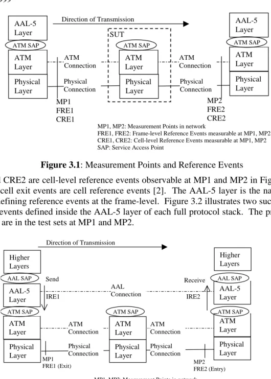
To describe frame-level performance parameters consistent with the general structure in ITU-T Recommendation I.350 [4], it is necessary to define frame-level reference events that are observable at measurement points in a network and then define relevant performance parameters based on these reference events. The measurement points are defined at physical locations in a network. The frame-level reference events are observable at these locations with suitable test sets; that is, the reference event definitions are based on physical layer test access. Figure 3.1 shows two such frame-level reference events that are labeled FRE1 and FRE2, and that are observable with suitable test equipment at the measurement points labeled MP1 and MP2, respectively. The SUT is tested either out-of-service in its network, or in a laboratory.
ATM Connection
ATM Connection
MP1, MP2: Measurement Points in network
FRE1, FRE2: Frame-level Reference Events measurable at MP1, MP2 CRE1, CRE2: Cell-level Reference Events measurable at MP1, MP2 SAP: Service Access Point
Direction of Transmission MP1 FRE1 CRE1 MP2 FRE2 CRE2 Physical Layer Physical Layer Physical Layer Physical Connection Physical Connection SUT ATM Layer AAL-5 Layer ATM SAP ATM Layer AAL-5 Layer ATM SAP ATM Layer ATM SAP
Figure 3.1: Measurement Points and Reference Events
CRE1 and CRE2 are cell-level reference events observable at MP1 and MP2 in Figure 3.1. Cell entry and cell exit events are cell reference events [2]. The AAL-5 layer is the natural place to consider defining reference events at the frame-level. Figure 3.2 illustrates two such frame-level reference events defined inside the AAL-5 layer of each full protocol stack. The protocol stacks illustrated are in the test sets at MP1 and MP2.
IRE1
Direction of Transmission
MP1, MP2: Measurement Points in network
FRE1, FRE2: Frame-level Reference Events measurable at MP1, MP2 IRE1, IRE2: (Internal) Reference Event internal to indicated protocol stacks SAP: Service Access Point
Physical Layer Physical Layer Physical Layer ATM Layer AAL-5 Layer Higher Layers ATM Layer AAL-5 Layer Higher Layers ATM Layer ATM Connection Physical Connection ATM Connection Physical Connection AAL Connection Send IRE2 Receive
ATM SAP ATM SAP ATM SAP
AAL SAP AAL SAP
MP1
FRE1 (Exit) MP2
FRE2 (Entry)
Figure 3.2: Frame-Level Internal and External Reference Events and Measurement Points
Reference events occur as relevant PDUs move across the protocol layer interface between the AAL-5 Convergence Sublayer (CS) and the AAL-5 Segmentation And Reassembly (SAR) sublayer. With respect to the indicated direction of transmission, these are labeled AAL-5 Internal Reference Event 1 (IRE1) and AAL-5 Internal Reference Event 2 (IRE2), respectively. Ideally, the IREs are the reference events one would like to measure to determine frame-level performance. However, since the IREs reference interfaces within the protocol stack, they are generally not physically accessible with test sets. Each FRE is defined to approximate an IRE,
and is observable at a MP with a suitable test set (i.e., the FRE is defined based on physical layer test access). The information content of FRE1 is, for practical purposes, the same as that of the corresponding IRE1 that generated it. The time of occurrence of FRE1, T1, lags behind the occurrence of IRE1 by a small and quantifiable amount. Similarly, the time of occurrence of FRE2, T2, leads the occurrence of IRE2 by a small and quantifiable amount.
Consistent with the structure provided by ITU-T Recommendation I.350 [4] requiring that performance parameters be defined in terms of performance-significant reference events that are observable at MPs, FRE1 and FRE2 shown in Figure 3.1 fulfill the requirement of observability at network measurement points MP1 and MP2 (located on the network side of these AAL-5 SAPs, and as close as practical to them), but IRE1 and IRE2 shown in Figure 3.2 do not.
Using the definitions of cell entry and exit events in [2], the following definitions for two frame-level reference events are proposed:
• Frame-level Reference exit Event (shown as FRE1): the occurrence of the cell exit event for the first user data cell of the frame;
• Frame-level Reference entry Event (shown as FRE2): the occurrence of the cell entry event for the last user data cell of the frame.
Observation of these frame-level reference events is possible because the MPs are located in a network. As shown in Figure 3.1, MP1 is located near the transmitting equipment and MP2 is located near the receiving equipment.
Test equipment at MP1 and MP2 would reconstruct the frames. Since each of these MPs is located near an ATM SAP, the cell transfer reference events CRE1 and CRE2 as defined in ITU-T Recommendation I.353 [5] are also observable, and hence, these MPs can be used to measure ATM cell transfer performance parameters. This coincidence of MPs for frame-level performance and for ATM cell transfer performance simplifies identifying the relations between these two types of performance parameters.
The frame-level performance parameters can be defined based on the above frame-level reference events. Following the approach of ITU-T Recommendation I.356 [6], appropriate frame transfer outcomes are defined based upon the occurrence of appropriate frame-level reference entry (FRE2) events at an MP2 near receiving equipment that corresponds to level reference exit (FRE1) events at an MP1 near transmitting equipment. Two frame-level reference events correspond if they are created by the same frame.
Again, in parallel with ITU-T Recommendation I.356 [6], a frame transfer outcome is defined as the occurrence at an MP2 of a FRE2 corresponding to the occurrence at an MP1 of a FRE1, within a specified time Tmax. A frame transfer outcome would generally be further classified by
certain criteria, such as whether or not the user information bits in the FRE2 match the user information bits in the corresponding FRE1.
Consistent with ITU-T draft Recommendation X.144 Amendment 1 Annex C [14], this approach will be demonstrated by applying it in sections 4.5.1 and 4.3.1 to develop proposed definitions for user information loss and user information delay performance parameters associated with frame transfer outcomes, respectively.
3.3. Reference Loads
A prerequisite for successful and repeatable performance testing is the definition of standard Reference Load Models (RLMs). RLMs are used to characterize test traffic in a well-defined manner for input into a System Under Test (SUT). With the use of well-defined RLMs specified as part of a test, the tester can run tests that are reproducible by other labs.
Given that this specification discusses measuring AAL-5 performance of ATM systems, it is fitting that a method for defining standardized frame RLMs should be defined for use in that testing.
The following sections define a consistent methodology for defining frame RLMs. This will allow testers to define test sources used for testing, without ambiguity.
3.3.1. Basic Framework of a Frame Reference Load Model
There are two basic logical components for frame RLMs to fully characterize their cell-level traffic patterns. These components are the frame sources and the cell multiplexer. The frame sources and multiplexer are only logical concepts that do not need to exist in any implementation. They can be considered virtual devices.
The frame source creates frames as sequences of cells with a well-defined pattern. Generally each source corresponds to a single VC. The multiplexer in turn describes how multiple frame sources, or perhaps cell sources as well, are put into a single output stream. For simplicity the input cell rate of a frame source to the multiplexer is defined to be equivalent to the output cell rate of the multiplexer.
Segmented Frames
ATM Cell Traffic Multiplexer 1 2 3 Source # cell Actual RLM
Figure 3.3: Logical model of a frame RLM
The multiplexer conceptually contains cell buffers for each source and some arbitration device. The arbitration device specifies how cells from multiple sources will be placed on the output stream. Conceptually, the actual RLM (well-defined traffic pattern) is what appears at the egress of the multiplexer. The multiple sources and multiplexer are used to characterize the RLM only, and need not exist in any implementation.
Using this framework requires the specification of two sets of parameters. These parameters are the frame source parameters for each source, and the multiplexer parameters.
3.3.2. Frame Source Parameters
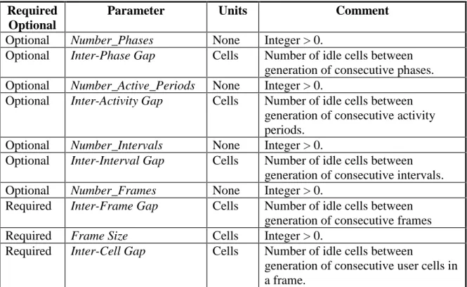
The following parameters can be used to characterize frame sources from a variety of applications. These parameters can be specified as having any mathematical, statistical or algorithmic distribution the author of a RLM feels is appropriate. This will allow for a wide range of useful RLMs.
The set of required parameters is the minimal subset to be used for defining a frame source. Theoretically, they can be used to define the majority of input RLMs, however for some sources this may be difficult. The optional parameters are defined recursively so that long term RLMs can be defined more simply.
Table 3.1: Frame Source Parameters Required
Optional
Parameter Units Comment
Optional Number_Phases None Integer > 0.
Optional Inter-Phase Gap Cells Number of idle cells between generation of consecutive phases. Optional Number_Active_Periods None Integer > 0.
Optional Inter-Activity Gap Cells Number of idle cells between generation of consecutive activity periods.
Optional Number_Intervals None Integer > 0.
Optional Inter-Interval Gap Cells Number of idle cells between generation of consecutive intervals. Optional Number_Frames None Integer > 0.
Required Inter-Frame Gap Cells Number of idle cells between generation of consecutive frames Required Frame Size Cells Integer > 0.
Required Inter-Cell Gap Cells Number of idle cells between
generation of consecutive user cells in a frame.
Interval
Interval
Interval
. . .
Interval
Active
Activity
Activity
. . .
Activity
Frame
Frame
Inter-
FG
Frame
. . .
Frame
Cell
Cell
Cell
. . .
Cell
Time
Time
IPG
Phase
. . .
Phase
Phase
Phase
IAG
IIG
CG
Figure 3.4: Relationship between Frame RLM source parameters
1. A test consists of one or more test phases. E.g., phases 1 and 2 might represent a test with one and ten traffic sources.
2. Each test phase (except the last) is followed by an inter-phase gap during which no traffic is generated.
3. A test phase consists of one or more periods of activity. E.g., a series of active periods might correspond to a series of traffic bursts.
4. Each active period (except the last) is followed by an inter-activity gap (idle period) during which no traffic is generated.
5. An active period consists of one or more characteristic intervals. E.g., intervals might correspond to the bin widths used by a self-similar traffic generator.
6. Each characteristic interval (except the last) is followed by an inter-interval gap during which no traffic is generated.
7. Traffic characteristics typically vary from one interval to the next. E.g., inter-frame gaps might vary among intervals, so that the inter-frame gap ~ exponential(10) in interval N and ~ exponential(15) in interval N+1.
8. Traffic characteristics typically do not vary within a characteristic interval. “Do not vary” does not imply that parameter values are constant. E.g., the length of the inter-frame gap during interval N is exponentially distributed with mean 10. However, parameter values are random variates drawn from this distribution and are not constant within interval N.
9. A characteristic interval consists of one or more frames.
10.Each frame (except the last) is followed by an inter-frame gap during which no traffic is generated.
12.Each cell (except the last) is followed by an inter-cell gap during which no traffic is generated.
13.Gaps at any level can be of length zero. E.g., phases 1 and 2 might represent a test with one and ten traffic sources, and with no pause during the transition.
3.3.3. Multiplexer Parameters
There is one parameter of interest to define the behavior of the multiplexer.
Arbitration Algorithm - Algorithm used to arbitrate amongst the various frame sources.
This algorithm must be a well-defined procedure that specifies which of the various sources with a cell to transmit, get to transmit a cell at any time. Included are any parameters that are required by the arbitration algorithm.
The author of the frame reference load model will define the arbitration scheme for the multiplexer device. The specification of this arbitration scheme must fully specify how all sources will be multiplexed so that the traffic pattern for any RLM is well defined at the cell-level.
The service rate of the arbitration device is assumed to be the output link rate, therefore idles occur in a RLM if and only if there are no sources with cells to send.
3.3.4. Definition of a Frame RLM
To properly define a frame RLM, the following must be specified: 1. All frame sources must be defined and numbered.
2. The multiplexer arbitration scheme must be specified to arbitrate between the sources.
To specify a frame source, the frame source parameters are defined as being distributed with well-defined distributions. These can be any mathematical, statistical or algorithmic distribution including constant. With proper definition of distributions for these parameters, a variety of useful frame sources can be constructed.
Section 3.3.5 and Appendix E contain example Frame RLMs.
To fully specify the multiplexer operation, the arbitration algorithm for the multiplexer must be stated.
Definition of these parameters specifies a well-defined RLM. It should be noted that these RLMs might be statistical in nature. If any of the parameters are based on statistical distributions, then the cell-level traffic patterns are statistically reproducible over time.
3.3.5. Example of the Definition of a Frame RLM
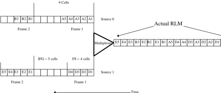
A hypothetical video compression frame stream could be defined to have the following characteristics:
1. There are two video frame sources with the following properties.
• A new data frame starts every 9 cell times.
• The data frames burst at line rate. That is the ICG = 0. 2. The 2 sources are multiplexed with round robin arbitration.
Therefore, the frame RLM would be defined with the following parameters:
Source 0
FS = Uniform(3,6) ICG = 0
IFGi= 9 - FSi i = Frame Number
Source 1
FS = Uniform(3,6) ICG = 0
IFGi= 9 - FSi i = Frame Number
Arbitration; Round Robin
Number_Of_Sources = 2. Round_Robin ( Number_Of_Sources ) { Current_Source = 0 while ( True ) { if ( Cell_To_Transmit ( Current_Source ) ) { Send_Cell ( Current_Source ) }
Current_Source = ( Current_Source + 1) mod Number_Of_Sources }
}
A1 A2 A3 A4 A5 B1 B2 B3 Multiplexer D1 D2 D3 D4 E1 E2 E3 E4 E5 A1 D1 A2 D2 A3 D3 A4 D4 A5 B1 E1 B2 E2 B3 E3 E4 E5 Example: Compressed video stream
Source 0
FS = Uniform(3,6) ICG = 0
IFGi= 9 - FSi i = Frame Number
Source 1
FS = Uniform(3,6) ICG = 0
IFGi= 9 - FSi i = Frame Number
Arbitration: Round Robin
Frame 1 Frame 1 Frame 2 Frame 2 Source 0 Source 1 FS = 4 cells IFG = 5 cells 9 Cells Actual RLM Time
Figure 3.5: Example Frame Reference Load Model of Two Video Sources
3.4. Test Configurations
Each Reference Load (RL) defined in Section 3.3 must be verifiable at the measurement point MP1, defined in Section 3.2. This specification does not (and should not) mandate any particular method for generating a RL. Some test configurations may include connections that are routed through the IUT several times by looping links (as a way to produce a traffic load on a large number of IUT input interfaces while using a small number of traffic generators – see Appendix B). In such cases, since the behavior of the IUT is formally unknown, so is the exact nature of the aggregate traffic passing through it. Therefore, the traffic pattern is unverifiable at each subsequent ingress to the IUT, as some of the input traffic comes from the IUT outputs.
Consider the following hypothetical example: we might attempt to measure the delay characteristics of two IUTs at an input port load of 98%. One IUT exhibits a CLR of 10-5 while the other 0.05. The load at the inputs of the IUT with the higher loss might be around 93% or lower while the load on the inputs of the other IUT would be much closer to the intended 98%.
Since the behavior of the two IUTs is different, there is a discrepancy between the test conditions under which the two IUTs are being observed.
The formal discrepancy of an unverifiable RL may be avoided by ensuring that those components of a test configuration that introduce dependencies on IUT performance are included in the definition of the system being tested. Therefore, should the test configuration incorporate looping configurations, the SUT should be defined to include the looping links.
This approach has the advantage of being consistent with the definitions of scaleable test configurations in Appendix B. It is the responsibility of the tester to verify that the test configuration does indeed produce the specified RL (for example by moving a cell stream analyzer around to each of the inputs and repeating the test).
A system with n ports can be tested for the following connection configurations (for connections internal to the SUT):
• n-to-n straight,
• n-to-(n−1) full cross,
• n-to-m partial cross, 1 ≤ m ≤ n−1,
• k-to-1, 1<k<n,
• 1-to-(n−1) multicast,
• n-to-(n−1) multicast.
Different connection configurations are illustrated in Figure 3.6, where each configuration includes one ATM switch with four ports, with their input components shown on the left and their output components shown the right.
In the case of n-to-n straight, input from one port exits to another port. This represents almost no path interference among the n VCCs. See Figure 3.6a.
In the case of n-to-(n−1) full cross, input from each port is divided equally to exit on each of the other (n−1) ports. This represents intense competition for the switching fabric by the n×(n−1) VCCs. See Figure 3.6b.
In the case of n-to-m partial cross, input from each port is divided equally to exit on the other m ports (1 ≤ m ≤ n−1). This represents partial competition for the switching fabrics by the n×m VCCs as shown in Figure 3.6c. Note that n-to-n straight and n-to-(n−1) full cross are special cases of n-to-m partial cross with m=1 and m=n−1, respectively.
In the case of k-to-1, input from k (1 < k < n) ports is destined to one output port. This stresses the output port logic. There are k VCCs as shown in Figure 3.6d.
In the case of 1-to-(n−1) multicast, all frames input on the one designated port are multicast to all other (n−1) ports. This tests single multicast performance of the switch. There is only one (multicast) VCC as shown in Figure 3.6e.
In the case of n-to-(n−1) multicast, input from each port is multicast to all other (n−1) ports. This tests multiple multicast performance of the switch. There are n (multicast) VCCs. See Figure 3.6f.
Note that a generalization of 1-to-(n-1) multicast and n-to-(n-1) multicast is m-to-(n-1) multicast with 1 ≤ m ≤ n.
Figure 3.6: Connection Configurations for Foreground Traffic
d. k-to-1: k VCCs; k=3
b. n-to-(n−1) full cross: n× (n−1)VCCs; n=4 a. n-to-n straight: n VCCs; n=4
e. 1-to-(n-1) multicast: one (multicast) VCC c. n-to-m partial cross: n×m VCCs; n=4, m=2
In In In In Out Out Out Out In In In In Out Out Out Out In In In In Out Out Out Out In In In In Out Out Out Out In In In In Out Out Out Out In In In In Out Out Out Out
3.4.1. Foreground Traffic
Before starting measurements, a number of VCCs (or VPCs), henceforth referred to as “foreground VCCs,” are established through the SUT. Foreground VCCs are used to transfer only the traffic whose performance is measured. That traffic is referred to as the foreground traffic.
Foreground traffic is specified by the type of foreground VCCs, connection configuration, service category, arrival patterns, frame length and input rate.
Foreground VCCs can be permanent or switched, virtual path or virtual channel connections, established between ports on the same network module on the switch, or between ports on different network modules, or between ports on different switching fabrics.
The list of foreground traffic characteristics and their possible values are now provided:
• type of foreground VCCs: permanent virtual path connections, switched virtual path connections, permanent virtual channel connections, switched virtual channel connections;
• foreground VCCs established: between ports inside a network module, between ports on
different network modules, between ports on different fabrics, some combination of
previous cases;
• connection configuration: one of the variants shown in Figure 3.6, e.g., n-to-m partial cross;
• service category: CBR, UBR, ABR, rt-VBR, nrt-VBR, and GFR (GFR is a frame-aware service category that does not apply to virtual path connections);
• frame size: 64, 1518, 9188, 65535 bytes or variable;
• inter-frame gap: constant, random;
• inter-cell gap: constant, random.
Values in bold indicate default traffic characteristics that, unless stated otherwise for a specific metric, it is recommended be used in performance testing.
The maximum foreground load (MFL) is defined as the sum of all physical link rates used for transmission of the foreground traffic, in the current switch configuration. Input rate of the foreground traffic is expressed in the effective bits/sec, counting only bits from frames, excluding the overhead introduced by the ATM technology and transmission systems.
3.4.2. Background Traffic
In connection configurations with multiple VCCs, it is possible to use some VCCs for foreground traffic and the others for background traffic. One particularly interesting case is when one VCC of the n-to-n straight configuration is used for foreground and the remaining n-1 VCCs are used for background. This will help study the effect of background traffic on the quality of service of the foreground traffic.
Background traffic characteristics that affect performance are the type of background VCCs, connection configuration, service category, arrival patterns (if applicable), frame length (if applicable) and input rate.
Like the foreground VCC, background VCCs can be permanent or switched, virtual path or channel connections, established between ports on the same network module on the switch, or between ports on different network modules, or between ports on different switching fabrics. To
avoid interference on the traffic generator/analyzer equipment, background VCCs are established in such a way that they do not use the input link or the output link of the foreground VCC in the same direction.
For an SUT with n ports, the background traffic can use (n–2) ports, not used by the foreground traffic, for both input and output. The port with the input link of the foreground traffic can be used as an output port for the background traffic. Similarly, the output port of the foreground traffic can be used as an input port for the background traffic. Overall, background traffic can use an equivalent of w=n–1 ports. The maximum background load (MBL) is defined as the sum of all physical link rates, except the one used as the input link for the foreground traffic, in the current switch configuration.
For background traffic, an SUT with n (=w+1) ports will support any one of the following background traffic connection configurations:
• w-to-w straight, with w background VCCs, (Figure 3.6a);
• w-to-(w–1) full cross, with w×(w–1) background VCCs. (Figure 3.6b);
• w-to-m partial cross, 1 ≤ m ≤ w–1, with w×m background VCCs. (Figure 3.6c);
• 1-to-(w–1) multicast, with one (multicast) background VCC. (Figure 3.6e);
• n-to-(w–1) multicast, with w (multicast) background VCC. (Figure 3.6d).
The list of background traffic characteristics and their possible values are now provided:
• type of background VCCs: permanent virtual path connections, switched virtual path connections, permanent virtual channel connections, switch virtual channel connections;
• background VCCs established: between ports inside a network module, between ports on
different network modules, between ports on different fabrics, some combination of
previous cases;
• service category:
UBR: priority equal to or lower than that of the foreground traffic; CBR: priority equal to or higher than that of the foreground traffic; rt-VBR, nrt-VBR, ABR, and GFR service categories are under study;
• arrival patterns: equally spaced frames, self-similar, random;
• frame size: 64, 1518, 9188, 65535 bytes or variable;
• inter-frame gap: constant, random;
• inter-cell gap: constant, random;
• input rate: 0, 0.5, 0.75, 0.875, 0.9375, 0.9687, … (i.e., 1 – 2-k, k = 0, 1, 2, 3, 4, 5,…) of MBL. Values in bold indicate default traffic characteristics that, unless stated otherwise for a specific metric, it is recommended be used in performance testing. Sometimes background traffic is not required (represented here by an input rate of “0”). When background traffic is required, the default input rate should be 0.875 of MBL. The UBR service category should be used if it is intended for the foreground traffic to have priority over the background traffic, and the CBR service category should be used for the inverse scenario.
Input rate of the background traffic is expressed in the effective bits/sec, counting only bits from frames excluding the overhead introduced by the ATM technology and transmission systems.
3.5. General Measurement Procedures
Before conducting performance tests, it is recommended that the port clocks are synchronized or locked together; otherwise, unstable results may be observed. In case of instability, one solution is to reduce the maximum load placed on the IUT to slightly below 100%. In this case, the load used should be reported.
Performance tests can be conducted under two conditions, remembering that the performance metric of interest is recorded only for the foreground traffic:
• without background traffic, or
• with background traffic.
The procedure to measure the performance metric in this case includes a number of test runs. A test run starts with the traffic being sent at a given input rate over the foreground VCCs. The average frame latency is constantly monitored. A test run ends and the foreground traffic is stopped when the average frame latency has not significantly changed (not more than 5%) during a period of at least 5 minutes. This ensures stability of the IUT.
3.6. Statistical Variations
For the given foreground and background traffic, performance metric results are recorded for p frames, according to the procedures described in Section 3.5. Here p is a parameter and its default is 100.
Let Ri be the result of the ith test. The sample mean, variance, standard deviation, and standard
error of the mean of the measurement are computed as follows: Mean = (Σ Ri) / p
Variance = (Σ(Ri – Mean)2) / (p–1)
Standard deviation = (Variance)1/2 Standard error = (Variance / p)1/2
Depending on the input traffic, the sample size p=100 may not be large enough to use the asymptotic technique or the measured data may be correlated. If the measurements of Ri for all i
are statistically independent, an unbiased estimate of the variance of the results is given above. However, in most measurement situations of practical interest, the measured results will not be statistically independent. In this case, techniques described in Appendix C.3 can be used to obtain an unbiased estimate of the variance of the results. Appendix C provides techniques for estimating confidence intervals. Appendix G provides simple recipes for standard statistical methods.
In some testing situations, it might be useful to compute and use statistics as soon as a measurement is obtained, rather than to compute them at the end of the test. The following recursive definition can be used to update statistics after each measurement:
measure R1
mean1 = R1 /* statistic from iteration 1 available for use */
variance1 = 0 /* variance1 is undefined; this statement is used to simplify the computation of variance2 */
measure Ri
meani = meani-1 + ((Ri - meani-1) / i)
variancei = ((1 - (1 / (i - 1))) x variancei-1) + (i x (meani - meani-1) 2
) standard_deviationi = (variancei)1/2
standard_errori = (variancei / i) ½
/* statistics from iteration i available for use */
}
3.7. Optional Traffic Management Functions and Procedures
The tester shall decide which subset of the available optional traffic management functions and procedures (from those listed in Section 5 of [2], or elsewhere) is to be implemented. Once the choice has been made, it shall be implemented consistently for the duration of the test, and reported along with the test results.
3.8. Reporting Results
A detailed description of the test configuration, including the SUT and RL, should always be attached to the test report. It should include details such as the number of ports, rate of each port, number of ports per network module, number of network modules, number of network modules per fabric, number of fabrics, maximum foreground load (MFL), maximum background load (MBL), software version, test equipment used, any optional performance enhancing schemes, traffic management functions and procedures that were implemented, and any other relevant information.
Values for the performance metric of interest, with corresponding input load are reported along with foreground (and background, if any) traffic characteristics. Appendix F provides two tables for reporting test results.
4.
Performance Metrics
4.1. Throughput
4.1.1. DefinitionsThere are three frame-level throughput metrics of interest to a user:
• Loss-less throughput - It is the maximum rate at which none of the offered frames is
dropped by the SUT.
• Peak throughput - It is the maximum rate at which the SUT operates regardless of frames
dropped. The maximum rate can actually occur when the loss is not zero.
• Full-load throughput - It is the rate at which the SUT operates when the input links are
loaded at 100% of their capacity.
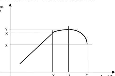
An example of a graph of throughput vs. input rate is shown in Figure 4.1. Level X defines the loss-less throughput, level Y defines the peak throughput, and level Z defines the full-load throughput.
The loss-less throughput is the highest load at which the count of the output frames equals the count of the input frames. The peak throughput is the maximum throughput that can be achieved
in spite of the losses. The full-load throughput is the throughput of the system at 100% load on input links. Note that the peak throughput may equal the loss-less throughput in some cases. Only frames that are received completely without errors are included in frame-level throughput computation. Partial frames and frames with CRC errors are not included.
Load (Input) Lossless Peak C B X Y X Z Full-Load Throughput (Output)
Figure 4.1: Peak, Loss-Less and Full-Load Throughput 4.1.2. Units
The preferred measurement for throughput is bits/sec. Bits/sec includes any overhead introduced by the SUT. Since for processing, the SUT may add headers and other information to the received data stream, its performance may be affected by the additional overhead it introduces. Also, for measurement purposes, it may not always be possible to identify and exclude overhead at the bit-level.
Alternately, frames/sec may be used, providing the frame size is specified in the results. Whichever measurement is used, it must be reported in the test results. Cells/sec, however, is not a good unit for frame-level performance, since the user normally doesn’t see the cells.
4.1.3. Measurement Procedures
During a given test run period, several test runs will need to be executed, and the total number of frames sent to the SUT and the total number of frames received from the SUT are recorded. The throughput (output rate) is computed based on the duration of a test run and the number of received frames.
If the input frame count and the output frame count are the same, then the input rate is increased, and the test is conducted again.
The loss-less throughput is the highest throughput at which the count of the output frames equals the count of the input frames.
The input rate is then increased even further. Although some frames will be lost, the throughput may increase till it reaches the peak throughput value. After this point, any further increase in the input rate will result in a decrease in the throughput.
The input rate is finally increased to 100% of the input link rates and the full-load throughput is recorded.
In the best case, where the frames are of fixed size and equally spaced, and the load is increased in steps, there is always measurement inaccuracy of at least the step size. If the frame size and spacing can vary, then the results can vary from one measurement to the next. Appendix C provides techniques for estimating confidence intervals for statistical parameters of interest, such as the means and/or variances of throughputs.
4.2. Frame Latency
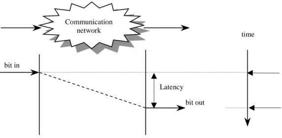
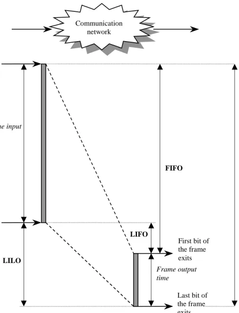
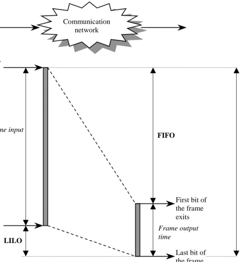
Two of the frame latency metrics of interest are First In Last Out (FILO), and Message-In Message-Out (MIMO). FILO indicates user perceived performance, whereas MIMO indicates latency that is introduced inherently by the SUT. Both are explained in Appendix A. Appendix A.12 also indicates other frame latency metrics of interest for additivity and end-to-end frame latency.
4.2.1. Definition
The previously defined frame reference events FRE1 and FRE2 and successful frame transfer outcome can be used to define a performance parameter for characterizing the information delay of the frame transfer outcome.
The FILO frame transmission delay parameter is defined as the time T2 of a FRE2 at MP2 minus the time T1 of a corresponding FRE1 at MP1, where the corresponding FRE2 and FRE1 are related as a successful frame transfer outcome. FILO is the information delay performance parameter that is directly measured. Other definitions of frame latency (e.g., MIMO) may be derived.
This definition excludes those FRE1 and FRE2 events associated with Corrupted Frame Transfer Outcomes, because such outcomes can be less reflective of normal user information delays. FILO latency is defined as follows:
FILO latency = Time between the first-bit entry and the last-bit exit MIMO latency is defined as follows:
MIMO latency = FILO latency – FILO0
where FILO0 (Nominal Frame Output Time) is defined as:
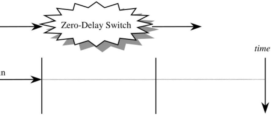
FILO0 = Time a frame needs to pass through the zero-delay switch
FILO0 can be calculated using the following procedure:
Initially FILO0 = 0 and time t is measured from the arrival of the first bit of the first cell. For
each cell with its first bit arriving at time t ⇒ FILO0 = max{t, FILO0} + CT.
Here CT is the larger of the