Regret bounds for transfer learning in Bayesian optimisation
Citation:
Shilton, Alistair, Gupta, Sunil, Rana, Santu and Venkatesh, Svetha 2017, Regret bounds for transfer
learning in Bayesian optimisation
, Proceedings of Machine Learning Research
, vol. 54, pp. 307-315.
© 2017, The Authors
Reproduced by Deakin University under the terms of the
Creative Commons Attribution Licence
Originally published online at:
http://proceedings.mlr.press/v54/shilton17a.html
Downloaded from DRO:
Alistair Shilton Sunil Gupta Santu Rana Svetha Venkatesh Deakin University, Australia Deakin University, Australia Deakin University, Australia Deakin University, Australia
Abstract
This paper studies the regret bound of two transfer learning algorithms in Bayesian opti-misation. The first algorithm models any dif-ference between the source and target func-tions as a noise process. The second algo-rithm proposes a new way to model the dif-ference between the source and target as a Gaussian process which is then used to adapt the source data. We show that in both cases the regret bounds are tighter than in the no transfer case. We also experimentally com-pare the performance of these algorithms rel-ative to no transfer learning and demonstrate benefits of transfer learning.
1
Introduction
Experimentation permeates human endeavour, pro-pelling us towards unexplored frontiers - new under-standing, formulation of novel materials, even biologi-cal elements of life. The process of experimentation in-volves conducting an experiment, measuring the qual-ity of output, then repeating the process with insights gained. This process and data acquired is inherently iterative, dynamic, small-scale, expensive and limited by resources of time, cost and even ideas. One of the main characteristics of experimentation is that knowl-edge is built over time through several sets of experi-ments that vary in setting - thus “similar” experimen-tal data is often available. For example, in machine learning when hyperparameter tuning has been per-formed in the past on a particular set of data then this should be transferable to hyperparameter tuning on a similar dataset.
Utilising such past and related (source) data to
im-Proceedings of the 20thInternational Conference on Artifi-cial Intelligence and Statistics (AISTATS) 2017, Fort Laud-erdale, Florida, USA. JMLR: W&CP volume 54. Copy-right 2017 by the author(s).
prove the output of the current experiment (target function) is a natural use for transfer learning. This needs to be incorporated into mechanisms that can handle limited data. Bayesian optimisation is an ex-citing sub-field of machine learning providing an ideal platform to estimate such functions from limited data, relating inputs to observed outputs via sequential op-timisation (Mockus, 2002; Snoek et al., 2012). It uses a Gaussian process (Rasmussen, 2006) to non-parametrically model the black-box function and con-verts the problem of optimising the unknown function to a problem of optimising a known surrogate function (acquisition function) constructed via the Gaussian process. Transfer of knowledge into such a Bayesian optimisation setting is desirable to solve the problem we are addressing. Though transfer learning is an es-tablished research area (Pan and Yang, 2010) for trans-ferring knowledge from past data, limited work has fo-cused on transfer learning for Bayesian optimisation (Bardenet et al., 2013; Yogatama and Mann, 2014). This paper examines the theoretical properties of transfer learning in Bayesian optimisation. Specifi-cally, we estimate the regret bounds of transfer learn-ing in Bayesian optimisation for two algorithms. The first algorithm, Env-GP (envelope-stretching Bayesian optimisation) (Joy et al., 2016), models any differences between the source and target functions as a noise pro-cess, stretchingthe noise envelope in the source data to fit it to the target, where the amount of stretch re-quired is proportional to the difference between them. By contrast the second algorithm, Diff-GP (difference-modelling Bayesian optimisation), directly models the difference between the source and target functions and then corrects the source data to match the target func-tion. To analyse the properties of Env-GP and Diff-GP by comparison to the non-transfer context we start with the work of Srinivas et al. (2010), which proves the statistical bound on total regret whilst using GP-UCB as a acquisition function
PrRT ≤√C1βTγTT +c0∀T ≥1≥1−δ,
where γT is the maximum information gain and c0 is a constant. We prove that both the maximum
infor-Regret Bounds for Transfer Learning in Bayesian Optimisation
mation gain γT and the noise dependent termC1 are decreased in the transfer learning context, and hence both Env-GP and Diff-GP are likely to find the opti-mum in fewer steps when source data is available. We demonstrate the efficacy of these algorithms, and show that the Diff-GP outperform the Env-GP as the source and target diverge. Our key contributions are:
• derivation of regret bounds for two transfer learn-ing algorithms in the context of Bayesian optimi-sation,
• presentation of a new transfer learning algorithm (Diff-GP), and
• experimental verification of algorithms on both simulated and real data.
2
Background
2.1 Gaussian Processes
A Gaussian Process (GP) is a random distribution over the set of smooth functions f : X ⊆ Rn → R on compactX denoted
f(x)∼GP (μ(x), k(x,x)),
where μ : X → R, μ(x) = E(f(x)) is the mean function of the Gaussian process; k : X × X → R,
k(x,x) = E((f(x)−μ(x)) (f(x)−μ(x))) is the kernel or covariance function. Without loss of gen-erality we may assume μ(x) = 0 and k(x,x) = 1 for all x ∈ X. The kernel k is a prior that encodes our underlying assumptions regarding smoothness of the distribution. A popular choice of kernel function is
k(x,x) = exp(−21ν2x−x
2
).
Given training data{(xat, yta)|t∈ZT}generated from
ya
t = f(xat) +a, where a ∼ N0, σa2
and ZT = {0,1, . . . , T−1}, the posterior overf is
f(x|yAT,XAT)∼ N μT(x), σ2T(x) , where μT(x) =kTAT(x) KAT+σ2aI −1 yAT, σ2 T(x) =k(x,x)−kTAT (x) KAT+σa2I −1 kAT(x) ; (1) and yAT = [ ya0 y1a . . . yaT−1 ]T, KAT = [ kxai,xaj ]i,j∈ZT, XAT = [ xa0 xa1 . . . xaT−1 ] and kAT (x) = [k(xia,x) ]Ti∈ZT. 2.2 Bayesian Optimisation
Letf(x) be a real-valued function over a compact do-main X ⊆Rn. Consider the problem
argmax
x∈X ⊆Rnf(x), (2)
where it is assumed thatf is computationally expen-sive to evaluate, and observations off may be affected by noise. Examples of such systems include optimising the performance of a machine learning technique for a given set of hyperparameters, or maximising the yield of a chemical reaction given temperature, pressure etc. The aim is to solve (2) using the minimum evaluations of f.
A popular approach to this problem is Bayesian optimisation (Jones et al., 1998). Bayesian opti-misation models f using a Gaussian process f ∼ GP (μ(x), k(x,x)) where without loss of generality it is assumed that μ= 0 and hence the Gaussian pro-cess is entirely specified by the kernel k. Bayesian optimisation is an iterative method that optimises a surrogate utility function (also known as acquisition function) whose role is to guide the optimiser to the optimum of the underlying function f in as few steps as possible.
The generic Bayesian optimisation function is as fol-lows:
1. Sett= 0.
2. Findxat = argmax
x∈X α(x|XAt,yAt).
3. Evaluateyat =f(xat).
4. Add new observation toAtasAt=At∪ {xat, yta}
5. Sett=t+ 1 and repeat from step 2 ift < T. where αis the acquisition function andT is the max-imum budget on the number of function evaluations. There are various acquisition functions e.g. probability of improvement (Kushner, 1964), expected improve-ment (Mockus, 2002) and Gaussian process upper con-fidence bound (GP-UCB) (Srinivas et al., 2012). The GP-UCB is especially amenable to theoretical analysis and is defined as
α(x) =μt−1(x) +√βtσt−1(x),
where βt are a sequence of constants. The first term in this acquisition function favours exploitation of pre-dicted maxima, and the latter exploration of unknown regions.
2.3 Experimental Design, Information Gain, and Regret Bounds
In experimental design (ED) (Chaloner and Verdinelli, 1995), information gain measures how informative a dataset {(xai, yai)|i∈ZT} generated from yta =
f(xat) +a, where a ∼ N0, σ2a
, is about a func-tion f. Information gain is defined to be the mutual information betweenf andyAT - that is,
I(yAT|f) =H(yAT)−H(yAT|f).
For a Gaussian distribution H(N(µ,Σ)) =
1
2log|2πeΣ|(Cover and Thomas, 2012), and hence
I(yAT|f) = 12logI+σa−2KAT.
In Bayesian optimisation, regret measures the distance from the optimal solution. For an optimiser following a sequence of pointsxa0,xa1, . . .the instantaneous regret at point tis
rt=f(x∗)−f(xat)≥0,
where x∗ is the true maximum of f. The cumulative regret up to instance T is
RT =t∈ZT rt.
In Srinivas et al. (2012) a number of statistical bounds are presented for the total regret in a GP-UCB con-text. These bounds take the form
PrRT ≤√C1βTγTT+c0∀T ≥1≥1−δ, (3)
where the sequenceβ0, β1, . . .is specified,C1 is a term
dependent on measurement noise, and
γT = max
AT⊂X | |AT|=TI
(yAT|fAT) (4) is the maximum information gain where f = [f(xa0), f(xa1), . . . , f(xaT−1)]. In the context of Bayesian optimisation our aim is to get (sufficiently close) to the optimum in the minimal number T of evaluations of f. The cumulative regretRT provides a measure of closeness to optimality after T steps. Thus the term√C1βTγTT provides a bound on
perfor-mance. In this paper we will demonstrate that both the maximum information gain γT and the term C1
may be decreased through the use of transfer learn-ing, enabling us to get closer to the optimum in fewer evaluations than in the non-transfer learning case.
3
Transfer Learning in Bayesian
Optimisation
Standard Bayesian optimisation starts with no obser-vations of the functionf and proceeds with a sequence
of test evaluations at pointsxa0,xa1, . . .to find the max-imum off. As such it suffers from a cold-start problem (Swersky et al., 2013; Joy et al., 2016). Transfer learn-ing is a means of overcomlearn-ing this problem and also of speeding up the convergence of the optimisation. In the transfer learning case it is assumed that there is a set of source data{xsi, yis|i∈ZNs}given a-priori,
where yis=f(xsi) +, ∼ N0, σ2. Limited work has focused on transfer learning in Bayesian optimisa-tion. Bardenet et al. (2013) built a transfer learning model under the rigid assumption that iff(x)≥f(y) for somex, y for the source function thenf(x)≥f(y) for the target function. This strong assumption rarely holds in practice, e.g. this assumption is violated for any two functions where one is a lagged version of the other. Yogatama and Mann (2014) built a transfer learning model to utilise past data assuming that the deviations of a function from its mean are transferable. Once again, this assumption holds only for highly sim-ilar functions.
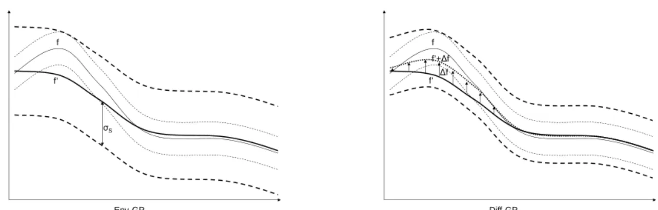
We present two approaches to transfer learning in this section. The first, envelope-stretching Bayesian op-timisation (Env-GP), was previously presented in Joy et al. (2016). The latter, difference-modelling Bayesian optimisation (Diff-GP), is presented here for the first time. The key difference between Env-GP and Diff-GP is illustrated in Figure 1:
• Env-GP: the Env-GP method models the source data using the target function by treating the dif-ference between the source and target functions as part of the noise model - that is,ysi =f(xsi) +s,
s∼ N0, σs2
, whereσs2> σ2is sufficiently large
to incorporate any source/target differences as a noise term.
• Diff-GP: the Diff-GP method explicitly models the difference between source and target functions as a Gaussian process and uses the prior obtained to construct a bias-corrected source data set. This bias-corrected source data may then be used di-rectly for the target without further stretching the envelope.
In sections 3.1 and 3.2, we describe both these meth-ods. Then in section 3.3, following Srinivas et al. (2012) we present a theoretical analysis of both meth-ods in terms of regret bounds, demonstrating how both proposed methods result in a tighter regret bound than the no transfer learning case.
Regret Bounds for Transfer Learning in Bayesian Optimisation f’ f σS Env-GP f’ f ∆f f’+∆f Diff-GP
Figure 1: Env-GP and Diff-GP operation. Env-GP (left figure) works by stretching the envelope about the source functionfto encompass the target functionf so that source data can be modelled in terms of the target function. Diff-GP (right figure), by contrast, constructs a bias-corrected source f+ Δf to better match the target.
3.1 Transfer Learning in Bayesian Optimisation 1: Env-GP
By definition ysi = f(xsi) + and f, f ∼
GP (μ(x), k(x,x)). It follows that there exists σs≥
σ such that the observationsys
i may be modelled by
ys
i =f(xsi) +s, wheres∼ N0, σs2
. The amount of “stretch” required to fit the source data to the target function depends on the magnitude of the difference betweenf−f between source and target functions. Given a set of source data {xsi, yis|i∈ZNs}
gener-ated as described and an appropriateσs, the
envelope-stretching Bayesian optimisation procedure (Env-GP) is:
1. Sett= 0.
2. Findxat = argmax
x∈X α(x|[XS,XAt],[yS,yAt]).
3. Evaluateyat =f(xat).
4. Add new observation toAtasAt=At∪ {xat, yta}
5. Sett=t+ 1 and repeat from step 2 ift < T. which differs from the standard Bayesian optimisation algorithm through the inclusion of source data at step 2. Note that fx| XS XAt , yS yAt ∼ Nμ˜t(x),σ˜t2(x) , where ˜ μt(x) = kS(x) kAt(x) T Q−1 yS yAt , ˜ σ2 t(x) =k(x,x)− kS(x) kAt(x) T Q−1 kS(x) kAt(x) Q= KS+σ2sI KSAt KTSA t KAt+σ2aI (5) and yS = [ y0s y1s . . . yNss−1 ] T, K S = [ kxsi,xsj ]i,j∈ZNs, XS = [ xs0 xs1 . . . xsNs−1 ], KSAt = [ k xsi,xaj ]i∈ZNs,j∈Zt, and kS(x) =
[ k(xsi,x) ]i∈ZNs. This method has been presented
in Joy et al. (2016), which also proposed a method for estimatingσsfrom observations.
3.2 Transfer Learning in Bayesian Optimisation 2: Diff-GP
Let {xsi, ysi|i∈ZNs} be the source data generated
by ysi = f(xsi) + , where ∼ N 0, σ2. Then f(x|XS,yS)∼ NμS(x), σ2 S(x) , where μS(x) = kTS(x) KS+σ2I−1yS, σ2 S(x) = k(x,x)−kTS(x) KS+σ2I−1kTS(x).
and the same covariance function has been used for both f andf. Let{xia, yai|i∈Zt}be the target data to time t. Definingg(x) =f(x)−f(x) and
Δyia(xai) = yia−μS(xai),
ΔyAt(XAt) = Δy0a Δya1 . . . Δyat−1 T, it follows that Δyai (x) = g(x) + g(x), where
g(x) ∼ N0, σ2a+σ2S(x) , and g(x|XAt,ΔyAt) ∼ NμDt(x), σ2Dt(x) , where μDt(x) =kTA t(x) KAt+σa2+σS2(x) I−1. . . . . .ΔyAt(XAt), σ2 Dt(x) =k(x,x). . . . . .−kTA t(x) KAt+ σ2 a+σ2S(x) I−1kAt(x),
and the subscript Dt indicates the value for the “dif-ference” function g(x). This allows us to construct the bias-corrected source data
xsi, ycsi,t(xsi) =yis+μDt(xsi)i∈ZNs
whereycsi,t(x) =f(x)+s,t(x) is the sum of the (noisy) source sampleysi =f(xsi) +and a correction factor
μDt(xsi) equal to the expected (mean) difference
be-tween target and source function atxsi and hence can be treated as a noisy sample of the target function; and
s,t(x) ∼ N0, σ2+σD2t(x)
. This bias-corrected source data may therefore be used for transfer learning in the Bayesian optimisation algorithm without addi-tional stretching of the envelope. We note that the target meanμDt(xsi) will change with each addition of
a new target observation, so the bias-corrected source data is a function of t, and moreover that there is some t-dependent envelope stretching built in to the bias-corrected source noise variance - i.e.
σ2
cs,t(x) =σ2+σ2Dt(x).
Given a set of source data the difference-modelling Bayesian optimisation procedure (Diff-GP) is:
1. Sett= 0.
2. Calculate the bias-corrected source data
xsi, yi,tcs(xsi) =yis+μDt(xsi)i∈ZNs 3. Find xat = argmax x∈X α(x|[XS,XAt],[yCSt,yAt]), whereyCSt = [y0cs,t(xs0). . . yNcss−1,t xsNs−1]T 4. Evaluate: yat =f(xat).
5. Add new observation toAtasAt=At∪ {xat, yta}
6. Sett=t+ 1 and repeat from step 2 ift < T. Note that fx| XS XAt , yCSt yAt ∼ Nμ˘t(x),σ˘t2(x) , where ˘ μt(x) = kS(x) kAt(x) T R−1 yCSt yAt ˘ σ2 t(x) =k(x,x)− kS(x) kAt(x) T R−1 kS(x) kAt(x) , R= KS+Σ2cs,t KSAt KTSA t KAt+σa2I (6) and Σ2cs,t= diagσcs,t2 (xs0), σ2cs,t(xs1), . . . , σ2cs,t xsN s−1 3.3 Regret Bounds
Our aim in this section is to study the effect of source data in the GP-UCB transfer learning scenario on the regret bound (3). Recall that the regret bound of in-terest has the form
Pr{RT ≤√C1βTγTT+c0∀T≥1} ≥1−δ
where the sequenceβ0, β1, . . .is specified,C1 is a term dependent on measurement noise, andγT is the max-imum information gain. We consider the impact of the source data separately on the maximum informa-tion gain γT and C1 and demonstrate that both are
decreased in the transfer learning case for both Env-GP and Diff-Env-GP, and hence that the bounding term
√C
1βTγTT on the convergence of the GP-UCB error
bound is tighter in the presence of source data.
Theorem 1. Let γT be the maximum information gain of the GP-UCB in the standard (no transfer learning) case and γ˜T the maximum information gain in the Env-GP (or Diff-GP) case, assuming Ns >0.
Then γ˜T < γT.
Proof. See appendix A.
Theorem 2. LetC1be the relevant term in the regret bound (3) of the GP-UCB in the standard (no transfer learning) case and C˜1 the same term in the Env-GP (or Diff-GP) case, assuming Ns>0. ThenC˜1< C1. Proof. See appendix A.
Theorems 1 and 2 together imply that
˜
C1βTγ˜TT < √
C1βTγTT, and hence, in both the Env-GP and
Diff-GP transfer learning algorithms we have a tighter re-gret bound in the transfer learning case,
Pr{RT ≤
˜
C1βT˜γTT+c0∀T ≥1} ≥1−δ, (7)
compared to the bound (3) for the non-transfer learn-ing case. This implies that both Env-GP and Diff-GP should be able to find the optimal solution more quickly than the standard (no transfer learning) case, on average.
Of course if the source function f is sufficiently dif-ferent from the target functionf, or the source points are located too far from the region wheref is optimal, then it may be assumed that there is no useful speed-up to be gained from the application of transfer learn-ing. For the Env-GP algorithm in this case we may expect that the envelope will need to be stretched sig-nificantly (soσswill be large). The following theorem shows that in such situations the benefits of transfer learning vanish:
Theorem 3. Using the notation of Theorems 1 and 2, lim ˜ σs→∞ ˜ C1βT˜γTT =√C1βTγTT ,
where σ˜s=σs in the Env-GP case, ˜σs =σcs,t in the
Diff-GP case.
Regret Bounds for Transfer Learning in Bayesian Optimisation
The response of the Diff-GP algorithm in such circum-stances is less clear. It may be that σcs,t(x) (likeσs
in the Env-GP case) will become large, in which case from Theorem 3 we may expect the benefit to vanish. However this depends entirely on whether Diff-GP is (a) able to learnthe difference between f andf and (b) whether the source data samples xsi are close to the optimum of the target function. For example, if the difference between f and f is simple - for exam-ple, if f(x) =f(x) + const - and the source samples are close to the target optimum then the Diff-GP al-gorithm may be expected to perform well even though
f−f
∞may be large.
4
Experimental Results
We consider two sets of experiments here. The first considers a simulated data set where we can control the similarity of the source and target functions. The target and source functions are
f(x) = exp(−12|x−μ1|2) and
f(x) = exp(−1
2|x−μ1| 2
),
where μ =μ+√sn, sis the shift factor and we have fixed the dimensionality ton= 2. By tuningsbetween 0 and 2 we are able to adjust the similarity between
f andf directly, wheres= 0 implies identical source and target functions and s = 2 gives very dissimi-lar functions. 20 source observations were generated uniformly randomly. Noise for both source and tar-get measurements was fixed with standard deviations
σ = σ = 0.1. For comparative purposes all simu-lations in the simulated data were run for T = 20 samples. The squared exponential kernel of the form
k(x,x) = exp(−2ν12x−x2) has been used for all
experiments with the length scaleν set to 0.1. Results for the simulated dataset are shown in Figure 2. As may be seen from these graphs both the Env-GP and Diff-GP algorithms outperformed the no-transfer-learning case for source shifts up to at least s = 0.5. It may be noted that for smalls(up to approximately
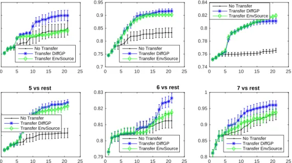
s= 0.2) the Env-GP and Diff-GP algorithm performed very similarly. However for moderate shifts (s = 0.4 ands= 0.5) Diff-GP outperforms Env-GP, which sup-ports our earlier discussion regarding the advantages of Diff-GP when the difference between source and target is moderate but simple in structure (or learnable). In our second experiment we performed tuning of hy-perparameters for a support vector machine. For this experiment we have used the 7-class UCI Image Seg-mentation Dataset (Lichman, 2013). The data was normalised to zero mean, unit variance on each fea-ture and split into 70/30 ratio for training and val-idation purposes. Our goal was to learn one-vs-rest
classifiers for all the classes. The first learning task (i.e. class 1-vs-rest) was used as a source function and all others (e.g. class 2-vs-rest) were separately treated as target functions. We used the LibSVM (Chang and Lin, 2011) toolbox, which has two hyperparameters for SVM using rbf kernel: kernel scaleγ and the cost pa-rameter C. Both were varied from [10−1,104]. The functions are learnt in the exponent space, with range [−1,4] for both the hyperparameters. The source func-tion was sampled on the full integer grid, whilst the target functions were optimized over the continuous space. Figure 3 shows the results of performance on the validation set vs evaluations for two transfer learning and the no-transfer learning (i.e. standard Bayesian optimization using only target data) algo-rithms. Evidently, within a fixed number of evalua-tions transfer learning algorithms (Env-GP and Diff-GP) are able to suggest better hyperparameters pared to no-transfer learning algorithm. When com-paring the two transfer learning algorithms, we note that in four out of six cases, the Diff-GP algorithm converged significantly faster than the Env-GP algo-rithm, resulting in higher accuracy performance with the budget of 20 iterations.
5
Conclusion
This paper has derived the regret bounds for two trans-fer learning algorithms in Bayesian optimisation us-ing GP-UCB as the acquisition function. The first al-gorithm (Env-GP) models the difference between the source and target functions as a noise process, whereas the second algorithm (Diff-GP) models the difference as a Gaussian process that is in turn used to correct targets in the source data. In addition to the regret bound the algorithms have been verified using both synthetic and real data to demonstrate the utility of these transfer learning methods. Our future work will examine the problem of how to derive similar trans-fer learning enabled tighter regret bounds for other acquisition functions such as expected improvement, predictive entropy search and so on.
A
Proof of Theorems 1-3
Theorem 1: The maximum information gain for the non transfer learning case is given by (4), where I(yAT|f) = 12logI+σa−2KAT. The distribution of the combined source/target datasets in the transfer learning case is yS fAT ∼ N 0 0 , KS+ ˜Σ2s KSAT KTSA T KAT ,
0 5 10 15 20 25 0 0.2 0.4 0.6 0.8 1 mean difference = 0.0 No Transfer Transfer DiffGP Transfer EnvSource 0 5 10 15 20 25 0 0.2 0.4 0.6 0.8 1 mean difference = 0.1 No Transfer Transfer DiffGP Transfer EnvSource 0 5 10 15 20 25 0 0.2 0.4 0.6 0.8 1 mean difference = 0.2 No Transfer Transfer DiffGP Transfer EnvSource 0 5 10 15 20 25 0 0.2 0.4 0.6 0.8 1 mean difference = 0.6 No Transfer Transfer DiffGP Transfer EnvSource 0 5 10 15 20 25 0 0.2 0.4 0.6 0.8 1 mean difference = 1.0 No Transfer Transfer DiffGP Transfer EnvSource 0 5 10 15 20 25 0 0.2 0.4 0.6 0.8 1 mean difference = 2.0 No Transfer Transfer DiffGP Transfer EnvSource
Figure 2: Simulated data results showing efficacy of transfer learning as a function of f−f. In each graph the x-axis shows evaluations and the y-axis shows the “best” solution found to that point. For all the graphs, the results are averaged over 20 optimization trials, each starting with 3 random observations from the target function. Error bars denote the standard errors.
0 5 10 15 20 25 0.72 0.74 0.76 0.78 0.8 0.82 2 vs rest No Transfer Transfer DiffGP Transfer EnvSource 0 5 10 15 20 25 0.7 0.75 0.8 0.85 0.9 0.95 3 vs rest No Transfer Transfer DiffGP Transfer EnvSource 0 5 10 15 20 25 0.74 0.76 0.78 0.8 0.82 0.84 4 vs rest No Transfer Transfer DiffGP Transfer EnvSource 0 5 10 15 20 25 0.75 0.8 0.85 0.9 5 vs rest No Transfer Transfer DiffGP Transfer EnvSource 0 5 10 15 20 25 0.79 0.8 0.81 0.82 0.83 6 vs rest No Transfer Transfer DiffGP Transfer EnvSource 0 5 10 15 20 25 0.8 0.85 0.9 0.95 1 7 vs rest No Transfer Transfer DiffGP Transfer EnvSource
Figure 3: Hyperparameter tuning results for SVM with rbf kernel on UCI Image Segmentation dataset. Hyperparameter-vs accuracy for Class 1 vs rest is used as a source function whilst all other one-vs-rest tun-ing problems are separately treated as target functions. In each graph the x-axis shows evaluations and the
y-axis shows the “best” solution found to that point. For all the graphs, the results are averaged over 20 op-timization trials, each starting with 3 random observations from the target function. Error bars denote the standard errors.
Regret Bounds for Transfer Learning in Bayesian Optimisation
where ˜Σ2s = σs2I in the Env-GP case and ˜Σ
2
s =
diagσ2cs,t(xs) in the Diff-GP case. It follows that,
in the transfer learning case, fAT ∼ N( ˜mAT,K˜AT),
where ˜ mAT = KTSAT KS+ ˜Σ2s −1 fAT, ˜ KAT = KAT −KTSAT KS+ ˜Σ2s −1 KSAT (8)
and by definition KA andKS are both positive
semi-definite. Assume without loss of generality that ˜
mAT =0. The information gain in the transfer
learn-ing case is therefore ˜I(yAT;f) = 12log|I+σa−2K˜AT|,
where it should be noted that the sequence of points
xa0,xa1, . . . ,xaT−1 will in general be different from the standard (non transfer learning) case. Using the fact that|A+B| ≥ |A|+|B|for positive definite matrices
A, B, ˜I(yA T;f) = 1 2log|I+σa−2KAT −. . . . . . σ−2 a KTSAT KS+ ˜Σ2sI −1 KSAT| ≤ 1 2logI+σa−2KAT. (9)
Using (9), it follows that, defining ˜γT as the maximum
information gain in the transfer learning case, ˜ γT = max AT⊂D:|AT|=T ˜I(yA T;fAT) = max AT⊂D:|AT|=T 1 2log|I+σa−2KAT −. . . . . . σ−2 a KTSAT KS+ ˜Σ2s −1 KSAT|
Using the Minkowski inequality on determinants of two positive definite matrices A and B, we have
|A+B| ≥ |A| +|B| > |A|. Assuming A = I+ σ−2 a KAT −σa−2KTSAT KS+ ˜Σ2s −1 KSAT and B = σ−2 a KTSAT KS+ ˜Σ2s −1
KSAT, we can write log|A|<
log|A+B| and thus conclude that ˜γT < γT. This completes the proof.
Theorem 2: In the original derivation of (3) in Srini-vas et al. (2012) the term C1 arises in the context of Lemma 5.4 in Srinivas et al. (2012). A key step in the proof of this lemma is the observation that
σ−2
a σ2t−1(xt)≤σ−a2k(xt,xt) ≤σ−2
a maxx∈Ak(x,x) =σ−a2,
which relies on the fact thatk(x,x) = 1 for allx∈ X. This leads to C1= log 8 (1+σ−2 a )maxx∈AT k(x,x) = 8 log(1+σ−2 a ).
In the context of transfer learning KA is replaced by ˜KA as defined by (8), the diagonals of which are
˜
k(xt,xt) =k(xt,xt)−kTS(xt) (KS+ ˜Σ2s)−1kS(xt)∈ (0,1). So, for transfer learning,
σ−2 a σt2−1(xt)≤σa−2k˜(xt,xt) ≤σ−2 a maxx∈A˜k(x,x) < σ−2 a ,
and hence, using the notation ˜C1 to distinguish from
the non transfer learning term C1,
˜ C1= log 8 (1+σ−2 a )maxx∈AT ˜ k(x,x)< C1,
which completes the proof.
Theorem 3: By (8) we have K˜AT = KAT − ˜ Σ−s2KTSA T( ˜Σ −2 s KS + I)−1KSAT. Noting that limσ˜s→∞( ˜Σ−s2KS + I) = I, it follows that limσ˜s→∞K˜AT = KAT. Hence it follows from the proofs of theorems 1 and 2 that ˜C1 →C1 and ˜γT →
γT, and the result follows.
References
Bardenet, R., Brendel, M., K´egl, B., and Sebag, M. (2013). Collaborative hyperparameter tuning. In
Proceedings of the 30th International Conference on Machine Learning (ICML-13), pages 199–207. Chaloner, K. and Verdinelli, I. (1995). Bayesian
exper-imental design: A review. Statistical Science, pages 273–304.
Chang, C.-C. and Lin, C.-J. (2011). LIBSVM: A li-brary for support vector machines. ACM Transac-tions on Intelligent Systems and Technology, 2:27:1– 27:27. Software available athttp://www.csie.ntu. edu.tw/~cjlin/libsvm.
Cover, T. M. and Thomas, J. A. (2012). Elements of information theory. John Wiley & Sons.
Jones, D. R., Schonlau, M., and Welch, W. J. (1998). Efficient global optimization of expensive black-box functions. Journal of Global optimization, 13(4):455–492.
Joy, T. T., Rana, S., Gupta, S. K., and Venkatesh, S. (2016). Flexible transfer learning framework for bayesian optimisation. In Advances in Knowl-edge Discovery and Data Mining, pages 102–114. Springer.
Kushner, H. J. (1964). A new method of locating the maximum point of an arbitrary multipeak curve in the presence of noise. Journal of Basic Engineering, 86(1):97–106.
Lichman, M. (2013). UCI machine learning repository. Mockus, J. (2002). Bayesian heuristic approach to global optimization and examples.Journal of Global Optimization, 22(1-4):191–203.
Pan, S. J. and Yang, Q. (2010). A survey on transfer learning. Knowledge and Data Engineering, IEEE Transactions on, 22(10):1345–1359.
Rasmussen, C. E. (2006). Gaussian processes for ma-chine learning.
Snoek, J., Larochelle, H., and Adams, R. P. (2012). Practical bayesian optimization of machine learning algorithms. In Advances in neural information pro-cessing systems, pages 2951–2959.
Srinivas, N., Krause, A., Kakade, S., and Seeger, M. (2010). Gaussian process optimization in the ban-dit setting: No regret and experimental design. In
Proc. International Conference on Machine Learn-ing (ICML).
Srinivas, N., Krause, A., Kakade, S. M., and Seeger, M. W. (2012). Information-theoretic regret bounds for gaussian process optimization in the bandit set-ting. IEEE Transactions on Information Theory, 58(5):3250–3265.
Swersky, K., Snoek, J., and Adams, R. P. (2013). Multi-task bayesian optimization. In Burges, C. J. C., Bottou, L., Welling, M., Ghahramani, Z., and Weinberger, K. Q., editors, Advances in Neural In-formation Processing Systems 26, pages 2004–2012. Curran Associates, Inc.
Yogatama, D. and Mann, G. (2014). Efficient transfer learning method for automatic hyperparameter tun-ing. In Proceedings of the 17th International Con-ference on Artificial Intelligence and Statistics (AIS-TATS).