MPGN – AN APPROACH FOR DISCOVERING
CLASS ASSOCIATION RULES∗
Iliya Mitov
Abstract. The article briefly presents some results achieved within the PhD project R1876Intelligent Systems’ Memory Structuring Using Multi-dimensional Numbered Information Spaces, successfully defended at Hasselt University. The main goal of this article is to show the possibilities of using multi-dimensional numbered information spaces in data mining processes on the example of the implementation of one associative classifier, called MPGN (Multi-layer Pyramidal Growing Networks).
1. Introduction. The knowledge discovery process consists of many steps and data mining is one of them [1]. Data Mining is the process of analyzing a large set of raw data in order to extract hidden information which can be
ACM Computing Classification System(1998): H.2.8, D.4.3.
Key words: Data mining, classification, associative classifiers, MPGN, multidimensional numbered information spaces, ArM 32.
*This article presents some of the results of the Ph.D. thesisClass Association Rule Mining
Using Multi-Dimensional Numbered Information Spacesby Iliya Mitov (Institute of Mathematics and Informatics, BAS), successfully defended at Hasselt University, Faculty of Science on 15 November 2011 in Belgium.
predicted [2]. The questions related to data mining present several aspects, such as: classification, estimation, clustering, associations, regularities, etc. From the whole data mining area we focus on classification algorithms and especially on associative classifiers, or so-called class-association rules (CAR) classifiers.
Associative classifiers appeared initially within the field of market basket analysis for discovering interesting rules from large data collections. As mentioned in [3], the five major advantages of associative classifiers can be highlighted:
– The training is very efficient regardless of the size of the training set; – Training sets with high dimensionality can be handled with ease and no
assumptions are made on dependence or independence of attributes; – The classification is very fast;
– Classification based on association methods presents higher accuracy than traditional classification methods [4] [5] [6] [7];
– The classification model is a set of rules easily interpreted by human beings and can be edited [8].
On the other hand, the process of creating classification models inevitably touches upon the use of appropriate access methods. We focus on the memory or-ganization called Multi-Dimensional Numbered Information Spaces which allows operating with context-free multidimensional data structures [9]. Our goal is to use such structures and operations in the implementation of one class association rule classifier MPGN in order to see the vitality of the idea of using context-free multidimensional data structures as a powerful tool for knowledge discovery.
The rest of the article is organised as follows: Section 2 makes a brief overview of the associative classifiers; Section 3 presents the algorithm of the proposed classifier MPGN; Section 4 draws attention to the program realization; Section 5 contains the results of the sensitivity analysis made with MPGN; and finally, in the conclusion, steps for future development are highlighted.
2. Associative classifiers. Generally the structure of CAR-classifiers consists of three major data mining steps: (1) Association rule mining; (2) Prun-ing (optional); and (3) Recognition.
The mining of association rules is a typical data mining task that works in an unsupervised manner. A major advantage of association rules is that they are theoretically capable of revealing all interesting relationships in a database.
But for practical applications the number of mined rules is usually too large to be exploited entirely. This is why the pruning phase is stringent in order to build accurate and compact classifiers. The fewer rules a classifier needs to approximate the target concept satisfactorily, the more human-interpretable is the result.
In 1998, CBA is introduced in [4], often considered to be the first asso-ciative classifier. During the last decade, various other assoasso-ciative classifiers were introduced, such as CMAR [5], ARC-AC and ARC-BC [10], CPAR [7], CorClass [11], ACRI [12], TFPC [13], HARMONY [14], MCAR [6], 2SARC1 and 2SARC2 [15], CACA [16], ARUBAS [17], etc.
2.1. Association Rule Mining. Several techniques for creating asso-ciation rules are used, mainly based on:
– Apriori algorithm [18] (used by CBA, ARC-AC, ARC-BC, ACRI, ARUBAS): Apriori makes multiple rounds over the data with patterns of length for 1 to k. Each pass consists of 2 steps – first: creating candidate patterns with length k; and second: remaining only patterns which support exceeds given support;
– FP-tree algorithm [19] (used by CMAR): FP-tree is an extended prefix-tree structure storing quantitative information about frequent patterns. Only frequent length-1 instances have nodes in the tree, and the tree nodes are arranged in such a way that more frequently occurring nodes will have better chances of sharing nodes than less frequently occurring ones; – FOIL algorithm [20] (used by CPAR): FOIL is a sequential covering
algo-rithm that learns first-order logic rules. It learns new rules one at a time, removing the positive examples covered by the latest rule before attempting to learn the next rule;
– Morishita & Sese Framework [21] (used by CorClass): It efficiently com-putes significant association rules according to common statistical measures such as chi-squared value or correlation coefficient.
Generating association rules can be made:
– from all training transactions together (applied in CBA, CMAR, ARC-AC); – for transactions grouped by class label (as is made in ARC-BC).
2.2. Pruning. In order to reduce the produced association rules, pruning in parallel with (pre-pruning) or after (post-pruning) creating association rules
is performed. Different heuristics for pruning during rule generation are used, mainly based on minimum support, minimum confidence and different kinds of error pruning [22]. At the post-pruning phase, criteria such as data coverage (ACRI) or correlation between consequent and antecedent (CMAR) are also used. During the pruning phase or at the classification stage, different ranking criteria for ordering the rules are used. The most common ranking mechanisms are based on the support, confidence and cardinality of the rules, but other tech-niques such as cosine measure and coverage measure (ACRI) also exist; we can mention amongst them:
– pruning by confidence: retain more general rules with higher accuracy: |R1|< |R2| and conf(R1) < conf(R2), then R1 is pruned (used in ARC-AC, ARCBC);
– pruning by precedence: special kind of ordering using “precedence” (CBA and MCAR);
– correlation pruning: statistical measuring of the rules’ significance using weighted χ2 (CMAR).
2.3. Recognition. Different approaches can be discerned in the recog-nition stage [17]:
– using a single rule (CBA); – using a subset of rules (CPAR); – using all rules (CMAR).
Different order-based combined measures for a subset or all rules can be applied also: select all matching rules; group rules per class value; order rules per class value according to some criterion; calculate a combined measure for the best Z rules; etc.
3. MPGN Algorithm. In [23] two associative classifiers are proposed: PGN and MPGN.
The algorithm of the PGN classifier is already presented in [24]. The PGN classifier has several advantages and experiments show very good benefits [23]. It possesses all advantages of CAR classifiers, such as creating a compact pattern set used in the recognition stage, easy interpretation of the results, and
very good accuracy for clear datasets. But one disadvantage is seen, connected with exponential growth of operations during the process of creating the pattern set.
In order to overcome this bottleneck, the MPGN algorithm is created. MPGN is an abbreviation of “Multi-layer Pyramidal Growing Networks of infor-mation spaces”. The main goal is to use a special kind of multi-layer memory structures called “pyramids”, which permits defining and realizing new opportu-nities.
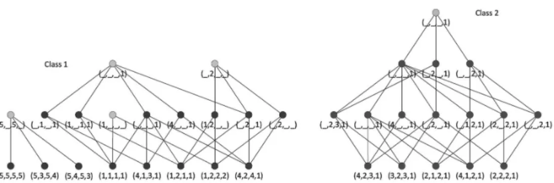
As an example we will use the following dataset for showing different steps of the MPGN algorithm (the separation of two classes in primary dataset is made only for increasing readability):
Class 1 R1: (1|5,5,5,5) R2: (1|5,3,5,4) R3: (1|5,4,5,3) R4: (1|1,1,1,1) R5: (1|4,1,3,1) R6: (1|1,2,1,1) R7: (1|1,2,2,2) R8: (1|4,2,4,1) Class 2 R9: (2|4,2,3,1) R10: (2|3,2,3,1) R11: (2|2,1,2,1) R12: (2|4,1,2,1) R13: (2|2,2,2,1)
3.1. Training process. The training process in MPGN consists of: – preprocessing step;
– generalization step; – pruning step.
3.1.1. Preprocessing step. MPGN deals with instances and patterns separately for each class. This allows the MPGN algorithm to be implemented for use on parallel computers which could be particularly helpful within the current trend of using cloud services and grid infrastructures.
The preprocessing steps aim to convert the learning set in a standard form for further steps. It consists of:
– discretization of numerical attributes [25];
– numbering the values of attributes and converting nominal vectors to nu-merical vectors.
3.1.2. Generalization step. The process of generalization is a chain of creating the patterns of the upper layer as intersection between patterns from the lower layer until new patterns are generated. For each class, the process starts from layer 1 that contains the instances of the training set. Patterns generated as intersections between instances of the training set, are stored in layer 2. Layer N is formed by patterns generated as intersections between patterns of the layer N-1. This process continues until further intersections are not possible.
During generalization, for every class a separate pyramidal network struc-ture is built. The process of generalization creates “vertical” interconnections between patterns from neighbourhood layers. These interconnections for every pattern are represented by a set of “predecessors” and a set of “successors”.
The predecessors’ set of a concrete pattern contains all patterns from the lower layer which were used in the process of its generalization. Thus in cases of different intersections generating the same pattern in the final outcome all patterns appearing in the intersection would be united as predecessors of the resulting pattern. The predecessors’ sets for instances of layer one are empty.
The successors’ set of a concrete pattern contains the patterns from the upper layer which are created from it. The successors’ sets of patterns on the top of the pyramid are empty. These patterns are called “vertices” of the corre-sponded pyramids.
One pattern may be included in more than one pyramid, but the vertex pattern belongs to one pyramid only.
It is possible for any pyramid to contain only one instance.
Figure 1 illustrates the result of the generalization step of MPGN for the example dataset. For simplifying the texts in the figures here and later patterns are presented only with value attributes. The class label is omitted as it is known from the pyramids in which pattern belongs. Light points denote vertices of the created pyramids.
3.1.3. Pruning steps. The pruning steps combine two different processes: – pre-pruning – in parallel with the generalization;
– post-pruning – pruning the contradictions.
Pre-pruning. During the generalization a huge amount of combinations
arises in big datasets. To restrict the combinatorial explosion different techniques can be applied. We use two different mechanisms for deciding which of the created patterns are to be included in the process of generalization.
Fig. 1. MPGN – Result of the generalization step on the example dataset The first mechanism allows excluding the patterns that are generated by few patterns from the lower layer. This is similar to support but here the direct predecessors rather than the primary instances are taken into account.
The other one tries to exclude the very general patterns from the be-ginning layers, using the presumption that these patterns will arise again in the upper layers. For this purpose, the ratio between the cardinality of the gener-ated patterns and the cardinality of the predecessor patterns can be used as a restriction.
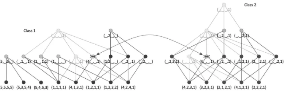
Post-pruning. Post-pruning is the process of iterative analysis of vertex
patterns of all pyramids from different classes and removing all contradictory vertex patterns. As a result, some of the most general patterns are deleted, because the vertices with the same bodies were available in other classes (and they also are deleted). The primary pyramids are decomposed to several sub-pyramids with a lower number of layers. The vertices of such sub-pyramids do not contradict vertices of pyramids of other classes.
Figure 2 shows the start of the process, where vertices of pyramids of class 1 and class 2 are compared and contradictory vertices as well as all successor equal patterns are destroyed.
The process of destroying contradictory vertices causes the arising of new vertices from the patterns of corresponding pyramids. For new vertices the search and destruction of contradictory patterns are applied again.
Fig. 3. Post-pruning – continuing the process
Figure 3 shows this next step on the example dataset. The process con-tinues iteratively since no contradictions between vertices of pyramids are found. In our case after the second traversing no new contradictions were found and the process of destroying pyramids stops.
Fig. 4. Final result of post-pruning
Figure 4 shows the final result of the post-pruning. In grey we show the destroyed parts of pyramids.
3.2. Recognition process. The instance to recognize is given by the values of its attributesQ= (?|b1, . . . , bn). Some of the values may be omitted. If
some attributes are numerical, the values of these attributes are replaced with the number of the corresponding discretized interval where the value belongs. The categorical attributes are also recoded with the corresponding number values.
Initially the set of classes that represent potential answers CS includes all classes: CS ={c|c= 1, . . . , M c}.
The recognition process consists of two main steps: – creating a recognition set for every class separately;
– analyzing the resulting recognition sets from all classes and making a deci-sion on which class is to be given as an answer.
3.2.1. Creating recognition set for each class. At this stage each class is processed separately.
The goal is to create for each class the recognition set which contains all patterns with maximal cardinality that have 100% intersection with the query.
The process starts from the vertices of all pyramids that belong to the examined class. Using the predecessor sets of the patterns in the recognition set each pattern is replaced with the set of their predecessors that have 100% inter-section with the query, if this set is not empty. After reducing the recognition set keeping only patterns with maximal coverage the process is iteratively repeated down to the layers until no new patterns appear in the recognition set.
The process of creating recognition set for each class can also be imple-mented on parallel computers.
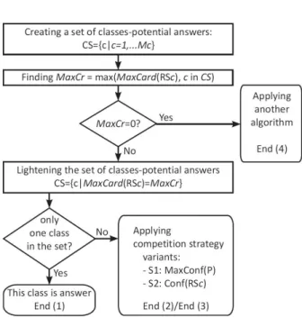
3.2.2. Analyzing results and making a final decision. Figure 5 shows the general schema of this step.
The result of the first step of the processing are the recognition sets for all classes RSc,c∈[1, . . . , Mc], which contain the patterns with maximal cardinality for this classM axCard(RSc),c∈[1, . . . , Mc] that have 100% intersection withQ. The goal is to find the class which contains the patterns with highest cardinality in its recognition set.
For this purpose, first the maximum of all maximal cardinalities of the recognition sets of classes from CS is discovered.
M axCr= max
c∈CSM axCard(RSc)
All classes that have not such maximal cardinality are excluded from the set CS.
Fig. 5. MPGN – comparative analysis between classes
After this step, if only one class remains in CS, then this class is given as an answer (End 1).
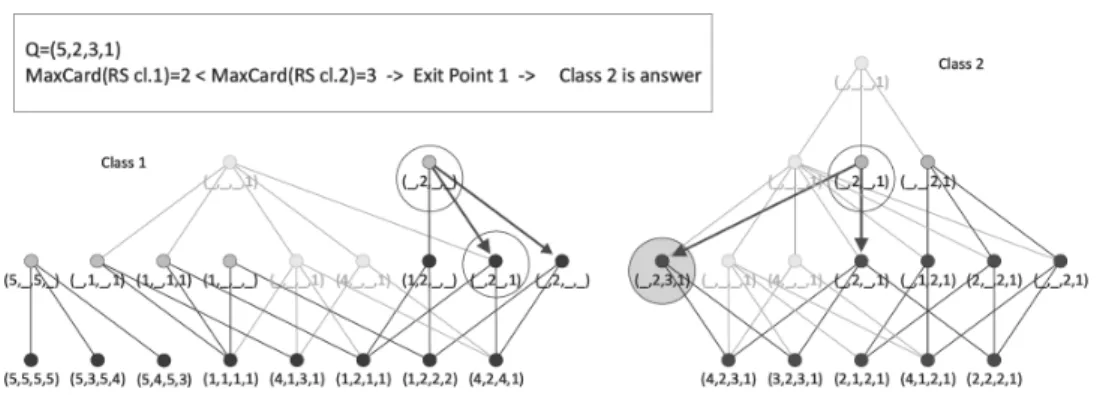
Let us see the recognition process over the example dataset for query
Q= (?|5,2,3,1), shown in Figure 6. Each class is examined separately.
Only vertex (1| ,2, , ) of class 1 matches the query. From its predecessors the pattern (1| ,2, ,1) match the query and has a greater cardinality, equal to 2. No match is found in its predecessors and process for class 1 stops.
In the case of class 2 the vertex (2| ,2, ,1) matches the query and its predecessor (2| ,2,3,1) also matches and has a greater cardinality, equal to 3.
As a result of comparison of maximal cardinalities between classes class 2 is given as the answer.
In the case when several classes exist with maximal cardinality M axCr
(i.e. Card(CS)>1), different strategies can be used to choose the best competi-tor. Here we will discuss two basic options:
– S1: choose from each class a single rule with maximal confidence within the class and compare it with others;
Fig. 6. Example of recognition in MPGN – Exit Point 1
that are covered by patterns from the recognition set of this class over the number of all instances of this class, and compare results.
Variant multiple classes-candidates: S1. The algorithm for the S1-option
can be summarized as follows:
– find the pattern with maximal confidence of each of the recognition sets of the classes in CS: M axConf(P ∈RSc) = max
P∈RSc(Conf(P)); – find the maximum of received numbers from all classes:
M axCn= max
c∈CSM axConf(P ∈RSc);
– reduce CS retaining only classes that have such maximum: CS = {c :
M axCard(RSc) =M axCr and M axConf(P ∈RSc) =M axCn};
– if only one class has such a maximum (End 2), this class is given as an answer; otherwise the class with maximal support from CS is given as answer. (End 3).
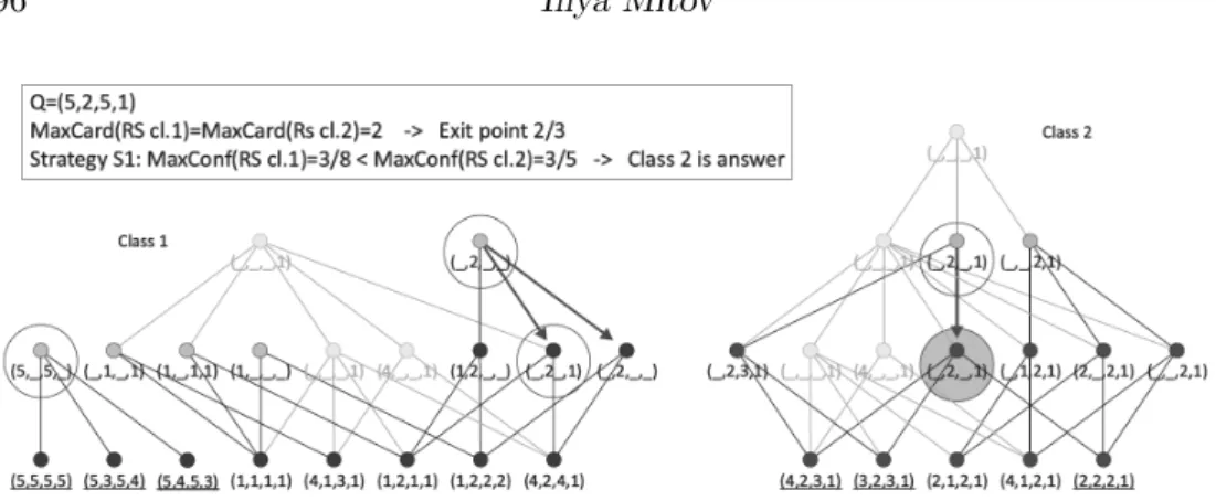
Let us see the behaviour of MPGN recognition: S1 strategy (Figure 7) on the case of queryQ= (?|5,2,5,1).
For class 1 the patterns that matched the query with maximal cardinality 2 are (1|5, ,5, ) and (1| ,2, ,1). For class 2 the pattern that matched the query with maximal cardinality again 2 is (2| ,2, ,1).
Because of the equality of the maximal cardinality we continue with find-ing the rule with maximal confidence within each class.
Fig. 7. Example of recognition in MPGN – Exit Point 2: Strategy S1
For class 1 the confidence of the pattern (1|5, ,5, ) is 3/8 (maximal for this class). For class 2 (2| ,2, ,1) has confidence 3/5. Following strategy S1 class 2 is given as answer.
Variant multiple classes-candidates: S2. This algorithm is similar to the
previous. The main difference is that instead of finding the pattern with maximal confidence of each of the recognition sets, here the “confidence of recognition set” is evaluated, i.e. the number of instances that are covered by patterns from the recognition set of this class over the number of all instances of this class and then results are compared. The rationale behind this is to take into account how many instances had been covered by all patterns from the recognition set. In practice this is the disjunction of the predecessors’ sets of Layer 1 (not direct predecessors) of the patterns that belong to RSc.
Let us see the behaviour of MPGN recognition: S2 strategy (Figure 8) on the case of the same queryQ= (?|5,2,5,1).
Following strategy S2 we found the confidences of the set of patterns that matches the query with maximal cardinality. They are correspondingly: 3/8+2/8=0.625 for class 1 and 3/5=0.600 for class 2. As a result class 1 is given as answer.
Variant: empty recognition sets. The worst case is when all recognition
sets were empty.
Here we create new recognition sets, including instances with maximal intersection percentage with the query.
M axIP erc(RSc, Q) = max
R∈RSc(IntersectP erc(R, Q)); RSc={R:IntersectP erc(R, Q)) =M axIP erc(RSc)}.
Find Conf(RSc) = |RSc|
|{instances of class c}|
The class that contains the set with maximal confidence is given as an answer. The reason is that a higher confidence is received because the rules are more inherent to this class. If two or more classes have equal confidence, than the class with maximal support is given as answer (End 4).
4. Program implementation. PGN and MPGN are implemented in the frame of the data mining environment PaGaNe. It uses the advantages of multi-dimensional numbered information spaces, provided by the access method ArM 32, such as the possibilities:
– to change searching with direct addressing in well-structured tasks; – to build growing space hierarchies of information elements;
– to build interconnections between information elements stored in the infor-mation base.
An important feature of the approaches used in PaGaNe is the replace-ment of the symbolic values of the objects’ features with integer numbers of the elements of corresponding ordered sets. All instances or patterns can be repre-sented by a vector of integer values, which may be used as a co-ordinate address in the corresponding multi-dimensional information space.
4.1. Preprocessing step. The preprocessing step is intended to con-vert the learning set to a standard form for further steps. It consists of: (1) dis-cretization of numerical attributes; (2) numbering the values of attributes; and (3) attribute subset selection.
4.1.1. Discretization. Because MPGN deal with categorical attributes, different discretization methods are implemented as a preprocessing step in Pa-GaNe. Special attention is paid to this process in [25].
4.1.2. Converting primary instances into numerical vectors. At this stage, the bijective functions between primary values and positive integers are generated. After that, the input instances are coded into numerical vec-tors, replacing attribute values with their corresponding numbers. The idea is to prepare data for direct use as addresses in the multi-dimensional numbered information spaces.
4.1.3. Attribute subset selection. The statistical observations on PaGaNe’s performance over the dataset can show that some attributes give no important information and the environment allows withdrawing such attributes from participation in further processing. The automatic subset selection is an open part of the implementation of PaGaNe and it is at the front of current and near-future investigation [26].
4.2. Training process. A very important aspect is that for each class there exists a separate class space, which has a multilayer structure called “pyra-mids”. All layers have equal structure and consist of “pattern-set” and “link-space”. For each class space a “vertex-set” also is maintained, which is used at the recognition stage.
4.2.1. Construction elements. Here we will define the structure of “pattern-set”, “link-space”, and “vertex-set”.
Pattern-set. Each pattern belongs to a definite class c and layer l. The
full denotation of pattern should be P(c, l) in order to make clear which class this pattern belongs to (note thatc is the class value of the pattern). We omitc
whenever it is clear from the context and denoteP(l). Whenl is also clear from the context we will denote only P.
All patterns of the class c which belongs to layer l form their pattern-set: P S(c, l) ={Pi(c, l)|i= 1, . . . , nc,l}. Each pattern P(c, l) from P S(c, l) have identifiers pid(P, c, l), or pid(P) for short when no ambiguity arises, which are natural numbers. The identifiers are created in increasing order of input of the patterns into pattern-set.
The process of generalization creates “vertical” interconnections between patterns from different (neighbourhood) layers. These interconnections for every pattern are represented by two sets of “predecessors” and “successors”.
The predecessors’ setP redS(Pi) contains the identifiers of patterns from the lower layer, which were used in the process of obtaining this pattern. The predecessors sets for instances of layer one are empty.
The successors’ setSuccS(Pi) contains the identifiers of patterns from the upper layer, which are created by this pattern. The successors’ sets of patterns on the top of the pyramid are empty. These patterns are called “vertices” of the corresponding pyramids.
One pattern may be included in more than one pyramid. The vertex pattern belongs only to one pyramid (they become top of the pyramids).
Link-space. The goal of the Link-space is to describe all regularities
be-tween attributes which are available in the classes. Links to the patterns which contain it are created for every value of each attribute, thus allowing to create a hierarchy of sets. The structure of this hierarchy is as follows:
– attribute value set: a set of patterns for given value of given attribute; – attribute set: a set of attribute value sets for given attribute;
– link-space (one): a set of all possible attribute sets.
The creation of the link-space uses the advantages of multi-dimensional numbered information spaces, especially the possibility to overcome searching by using direct pointing via coordinate addresses.
Below we will focus our attention on the link-space, which becomes a key element of accelerating the creation of new patterns as well as searching patterns satisfying the queries.
Letc be one number of the examined class and lbe the number of given layer ofc:
– attribute value set V S(c, l, t, v), v = 1, . . . , nt is a set of all identifiers of instances/patterns for classc, layer l, which have valuev for the attribute
t: V S(c, l, t, v) ={pid(Pi, c, l), i= 0, . . . , x|ai t=v};
– attribute set AS(c, l, a) for a concrete attribute a= 1, . . . , n is a set of at-tribute value sets for classc, layerland attributet:AS(c, l, t)={V S(c, l, t,1), . . . , V S(c, l, t, nt)}, where nt is the number of values of attribute t;
– link-space LS(c, l) is a set of all possible attribute sets for classcand layer
l: LS(c, l) ={AS(c, l,1), . . . , AS(c, l, n)}.
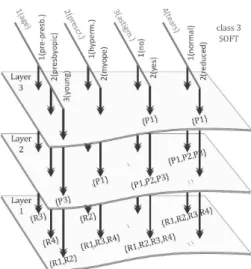
In Figure 9, the visualization of class 3 of the “Lenses” dataset [27] during the creation of the patterns is shown.
Such information is stored in ArM-structures by a very simple convention – the attribute value sets V S(c, l, t, v) is stored in the points of the ArM-archive
Fig. 9. Visualization of link-spaces
using the corresponding address (4, c, l, t, v), where 4 is the dimension of the ArM space, c is the number of the class, l is the number of the layer, t is the number of the attribute and v is the number of the corresponding values of the given attribute. The disposition of link-spaces in ArM-structures allows very fast extraction of available patterns in the corresponding layer and class.
Vertex-set. The vertex-set contains information about the patterns that
have no successors in the pyramids of the corresponding class.
V rS(c) ={pid(Pi, c, l) |i= 1, . . . , nc,l; l= 1, . . . , lmax:SuccS(Pi) =∅}. 4.2.2. Generation of the rules. The process of rule generation is a chain of creating the patterns of the upper layer as an intersection between patterns from the lower layer until new patterns are generated.
Each instance R = (c|a1, . . . , an) from the learning set is included into the pattern-set of the first layer of its class c: R∈P S(c,1).
Starting from layer l= 2 the following steps are made:
(1) Creating the link-space of the lower layerl−1 of classcby adding the identifiers of patterns Pi ∈ P S(c, l−1), i = 1, . . . , nc,l−1 to the attribute value sets of the values: pid(Pi) ∈ V S(c, l−1, ki, ai
k), k = 1, . . . , n. Note that these sets became ordered during creation;
(2) The set of patterns which are intersections of the patterns of the lower layer Pi ∩Pj, Pi, Pj ∈ P S(c, l−1), i, j = 1, . . . , k
c,l−1, i 6= j is created. The algorithm for creating this set is given below;
(3) If patterns are not generated (i.e. P S(c, l) ={ }), then the process of generating the rules for this class stops;
(4) On the basis of obtaining a set of patterns, the pattern-setP S(c, l) of layer lis created as follows:
– Each pattern from the receiving set of patterns is checked for existence in theP S(c, l);
– If this pattern does not exist in P S(c, l), it receives an identifier which is equal to the next number of identifiers of the patterns in the pattern-set; the pattern is added at the end of the pattern-set; and its predecessor-set is created with two pairs{(pid(Pi), l−1), (pid(Pj), l−1)};
– If this pattern already exists in P S(c, l), its predecessor-set is formed as a union of the existent predecessor-set and{(pid(Pi), l−1), (pid(Pj), l−1)}. (5) For each pattern from layer l check for existence the same pattern in lower layers (from layer l−1 to layer 2). If such a pattern exists, then it is removed from the pattern-set and corresponding link-space of the lower layer and the predecessor-set of the current pattern is enriched with the predecessor-set of the removed pattern (by union).
(6) Incrementing layer l and repeating the process.
As a result, for every class a separate pyramidal network structure is built. Each pyramid is described by a predecessor-set and a successor-set of patterns in neighbour layers.
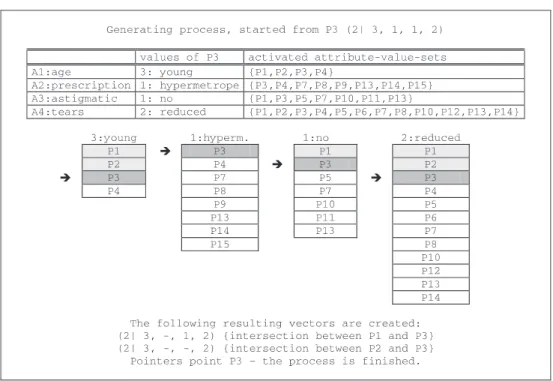
4.2.3. Generating the set of patterns which are intersections of patterns from the lower level. For restricting the exponential growth of intersections two parameters are included in program implementation:
– L1 (from 0 to 100) – percentage of reduced patterns per layer;
– L2 (from 0 to 100) – minimal ratio in percent of the cardinality of the generated pattern to the maximal cardinality of patterns in lower layer.
The process of generating the intersections of the patterns from a given pattern-set P S(c, l) loops through each pattern Pi ∈P S(c, l).
For this patternPi = (c|ai
1, . . . , ain) the generation of possible patterns is: (1) An empty set of resulting patterns is created;
(2) For all attribute valuesai1, . . . , aindifferent from “–” ofPi we take the corresponding attribute-value-sets V S(c, l, ki, ai
k), i= 1, . . . , n. The numbers of identifiers of the patterns in these sets are ordered.
è è
è
è
Fig. 10. Visualization of the process of generating a set of patterns (3) All extracted attribute-value-sets are activated.
(4) From each of them the first identifier is given.
(5) While at least one attribute-value-set is active, the following steps are made:
– Assign the initial values of the resulting pattern: V = (c|−,−, . . . ,−); – Locate the minimal identifier pid(Pj) from all active attribute-value-sets; – If pid(Pj) =pid(Pi), then this attribute-value-set is deactivated;
– All active attribute-value-sets V S(c, l, kj, aj
k), j = 1, . . . , kc,l, for which
pid(Pj) is the current identifier, cause filling of the corresponding attribute valueaik of kth attribute inV. For these sets the next identifier is given; – If |V|>0 and min |V| |Pi|, |V| |Pj|
> L2, this pattern is included into the set of resulting patterns with additional information containing pid(Pi) and
pid(Pj).
At the end the patterns in the created pattern set are sorted by the num-ber of their predecessors and L1% of them with fewer predecessors are removed.
4.3. Recognition process. The record to be recognized is represented by the values of its attributes Q = (?|b1, . . . , bn). Some of the features may be omitted. The classification stage consists of several steps:
(1) Using the service attribute-values-space, the system takes correspond-ing attribute value sets for all attributes b1, . . . , bn as well as the attribute value sets for “–” as a value of each attribute.
(2) The union of these sets gives a set of possible classes{c1, . . . , cy}, which the record may belong to. This approach decreases the amount of information needed for pattern recognition.
(3) All classes which are presented in this union{c1, . . . , cy}are scanned in parallel. For each classcx and for each layer of class space of cx the following steps are done:
– For all attribute values b1, . . . , bn different from “–” of Q we obtain the corresponding attribute value sets from the link-space of classcx of current layer;
– The intersection between all these sets is made. As a result a recognition set of candidate patterns is created. If this set is empty, the target class is a class with maximal support;
– For each pattern P which is a member of the recognition set calculate
IntersectP erc(P, Q).
(4) From all recognition sets of the classes and layers the patterns with maximal cardinality are found.
(5) These recognition sets are reduced by excluding the patterns whose cardinality is less than the maximal cardinality. The new set of classes-potential answers {c1, . . . , cy′} contains only classes whose recognition sets are not empty.
(6) If only one class is in the set of classes-potential answers, then this is the target class and the process stops.
(7) Otherwise, if this set is empty, we produce again a primary set of classes-potential answers {c1, . . . , cy′} = {c1, . . . , cy} and the process continues with examining this set.
(8) Examine{c1, . . . , cy′}:
– for each class which is a member of this set, the number of instances with maximal intersection percentage with the query is found and the ratio be-tween these numbers and all instances in the class is calculated;
– the maximum of intersection percentages from all classes is determinated and in the set{c1, . . . , cy′} only classes with this maximal percentage and
maximal ratio is left;
– if {c1, . . . , cy′}contains only one class, this class is given as answer.
Other-wise the class of{c1, . . . , cy′}with maximal instances is given as an answer.
And the process stops.
We can assume that the possibilities for keeping numerous created pat-terns in a manageable way allow using this environment to test different kinds of recognition models.
Here the algorithm of recognition strategy S1 was described. The al-gorithm for strategy S2 differs only in points 4 and 5, where the criterion for selection of classes-candidates is the so-called “confidence of recognition set”.
5. Sensitivity analysis. We made different experiments for studying the specific behaviour of the proposed algorithm and for comparing the results of MPGN and other classifiers that use similar classification models. For the exper-iments we used 25 datasets from UCI Machine Learning Repository [27], which contain different numbers of classes and different types of attributes: audiol-ogy, balance scale, blood transfusion, breast cancer wo, car, cmc, credit, ecoli, forestfires, glass, haberman, hayes-roth, hepatitis, iris, lenses, monks1, monks2, monks3, post-operative, soybean, tae, tic tac toe, wine, winequality-red, and zoo.
In order to receive more stable results we applied a 5-fold cross-validation technique. For achieving equality of data used for different classifiers we exported learning sets and examining sets from PaGaNe as input files in other programs.
We compared the proposed classifiers PGN and MPGN with some of those implemented in Weka [28] and LUCS-KDD Repository [29]. In the experiments we made a comparison with CMAR (thresholds: 1% support and 50% confidence) [5] as representative of other associative classifiers (implemented in the LUCS-KDD Repository), OneR [30] and JRip (Weka implementation of RIPPER [31]) as representatives of decision rules classifiers, and J48 (Weka implementation of C 4.5 [32]) and REPTree [28] as representatives of decision trees. The comparisons are two-fold’ measuring: (1) overall accuracy; and (2) F-measure results.
5.1. Examining the Exit Points of MPGN. During the design of MPGN we believe that the pyramidal network contains enough information to classify. So we expect that most unseen cases can be classified by using the
structure. In other words we expect that in the recognition phase only few cases will have an empty recognition set. We are also interested in how many cases have a recognition set with one class and how many cases have multiple conflicting classes. The latter cases can be classified on the basis of confidence or support. At the second step of the recognition phase MPGN can fail in different situations:
– only one class is a class-candidate – we mark this case as Exit point 1; – several classes are class-candidates. In this case two strategies are suggested
in order to choose the best competitor: S1: from each class choose a single rule with the maximal confidence within the class and compare with others; and S2: find “confidence of recognition set”, i.e. the number of instances that are covered by patterns from the recognition set of this class over the number of all instances of this class and compare results. In both strategies the cases are classified based on maximal confidence (Exit point 2) or maximal support (Exit point 3);
– empty recognition sets – in this case another algorithm is used – the Exit point 4.
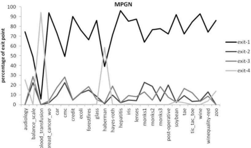
Figure 11 illustrates the percentage of different kinds of exits. In most cases the recognition leads to exit 1, which means that applying MPGN is worth-while.
We examine in more detail the two strategies for multiple classes (Exit points 2 and 3). Figure 12 presents the scatter plot of the obtained accuracies for
Fig. 12. Scatter plot of the obtained accuracies for MPGN-S1 and MPGN-S2
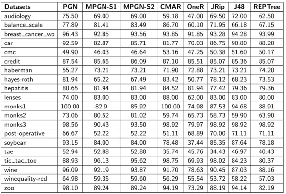
Table 1. Percentage of overall accuracy of examined datasets for PGN, MPGN-S1, MPGN-S2, CMAR, OneR, JRip, J48, and REPTree
Datasets PGN MPGN-S1 MPGN-S2 CMAR OneR JRip J48 REPTree
audiology 75.50 69.00 69.00 59.18 47.00 69.50 72.00 62.50 balance scale 77.89 81.41 83.49 86.70 60.10 71.95 66.18 67.15 breast cancer wo 96.43 92.85 93.56 93.85 91.85 93.28 94.28 93.99 car 92.59 82.87 85.71 81.77 70.03 86.75 90.80 88.20 cmc 49.90 46.03 46.64 53.16 47.25 50.38 51.60 50.17 credit 87.54 85.65 86.09 87.10 85.51 85.07 85.36 85.07 haberman 55.27 73.21 73.21 71.90 72.88 73.21 73.21 74.20 hayes-roth 81.94 65.22 67.49 83.42 50.77 78.12 68.23 73.53 hepatitis 80.65 81.94 81.94 84.52 81.94 77.42 79.36 79.36 lenses 74.00 83.00 83.00 88.00 62.00 83.00 83.00 80.00 monks1 100.00 82.9 85.92 100.00 74.98 87.53 94.68 88.91 monks2 73.06 80.52 81.02 59.74 65.73 58.73 59.90 63.90 monks3 98.56 90.43 93.50 98.92 79.97 98.92 98.92 98.92 post-operative 66.67 52.22 52.22 51.11 68.89 70.00 71.11 71.11 soybean 93.15 84.00 84.00 78.48 37.44 85.35 87.64 78.18 tae 52.94 52.88 52.88 35.74 45.76 34.43 46.97 40.43 tic tac toe 88.93 96.13 95.62 98.75 69.93 98.02 84.23 80.37 wine 96.09 92.19 93.87 91.70 78.63 90.45 87.03 88.16 winequality-red 64.98 59.35 59.60 56.29 55.54 53.72 58.22 57.03 zoo 98.10 89.24 89.24 94.19 73.29 88.19 94.14 82.19
both strategies. We can conclude that Strategy 2 has a mean accuracy of 49% and Strategy 1 has a mean accuracy of 46%. The Friedman test showsχ2F = 2.56,
α0.05= 1.960, which means that the S2 statistically outperforms MPGN-S1.
In conclusion, the analysis of different recognition parts taught us that the initial idea of the PaGaNe algorithms works well and that for many cases the recognition set contains only one and the correct class.
5.2. Comparison with overall accuracy. In Table 1 the obtained results for the overall accuracy are shown.
We use the Friedman test to detect statistically significant differences between the classifiers in terms of average accuracy [33]. The Friedman test is a non-parametric test, based on the ranking of the algorithms on each dataset instead of the true accuracy estimates. We use Average Ranks ranking method, which is a simple ranking method, inspired by Friedman’s statistic [34].
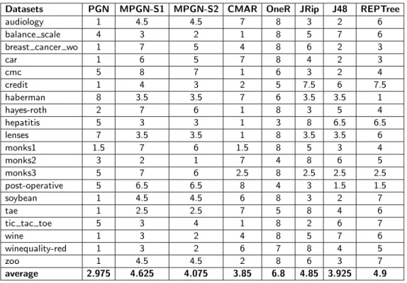
In order to apply the Friedman test to measure the statistical dissimilarity of different classifiers we ranked the results (Table 2).
Table 2. Ranking by accuracy of examined classifierscentering
Datasets PGN MPGN-S1 MPGN-S2 CMAR OneR JRip J48 REPTree
audiology 1 4.5 4.5 7 8 3 2 6 balance scale 4 3 2 1 8 5 7 6 breast cancer wo 1 7 5 4 8 6 2 3 car 1 6 5 7 8 4 2 3 cmc 5 8 7 1 6 3 2 4 credit 1 4 3 2 5 7.5 6 7.5 haberman 8 3.5 3.5 7 6 3.5 3.5 1 hayes-roth 2 7 6 1 8 3 5 4 hepatitis 5 3 3 1 3 8 6.5 6.5 lenses 7 3.5 3.5 1 8 3.5 3.5 6 monks1 1.5 7 6 1.5 8 5 3 4 monks2 3 2 1 7 4 8 6 5 monks3 5 7 6 2.5 8 2.5 2.5 2.5 post-operative 5 6.5 6.5 8 4 3 1.5 1.5 soybean 1 4.5 4.5 6 8 3 2 7 tae 1 2.5 2.5 7 5 8 4 6
tic tac toe 5 3 4 1 8 2 6 7
wine 1 3 2 4 8 5 7 6
winequality-red 1 3 2 6 7 8 4 5
zoo 1 4.5 4.5 2 8 6 3 7
The null hypothesis critical value for the Friedman test isα0.05= 14.067; in our case χ2F = 29.492, which means that the null-hypothesis is rejected, i.e. the classifiers are statistically different. We see that PGN has the best overall performance among the examined classifiers. MPGN is competitive with J48, JRip and REPTree.
5.3. Analyzing F-measures on some multi-class datasets. The overall accuracy of a particular accuracy may be good in some cases, and yet it might not be able to recognize some of the class labels for different reasons – small percentage of presence of given class label, confusion with another, etc. We make the experiments over datasets with two particular characteristics – too many class labels, and unbalanced support of different class labels – such are the Glass and Soybean datasets. We choose the F-measure as the harmonic mean of recall (measure of completeness) and precision (measure of exactness).
Glass dataset. The Glass dataset has 6 class labels with very uneven
distribution between them: 2#: 35.51%; 1#: 32.71%; 7#: 13.55%; 3#: 7.94%; Table 3. Percentage of F-measure from tested classifiers for the Glass dataset
Class labels PGN MPGN-S1 MPGN-S2 OneR CMAR Jrip J48 REPTree
2# (35.5%) 80.3 81.6 82.2 57.5 79.7 67.9 78.1 75.2 1# (32.7%) 80.3 81.1 81.1 64.4 80.5 69.0 76.5 70.1 7# (13.6%) 89.7 89.7 89.7 53.8 90.3 85.7 84.2 67.8 3# (7.9%) 51.9 59.5 57.9 0.0 38.5 16.0 29.6 34.5 5# (6.1%) 58.1 69.2 69.2 0.0 64.0 53.8 64.5 21.1 6# (4.2%) 88.9 94.1 94.1 0.0 77.8 60.0 55.6 80.0
5#: 6.07%; 6#: 4.21%.
Table 3 and Figure 13 present the F-measure for each class label from different classifiers.
As we can see PGN and MPGN have good performance for each of the class labels. For instance, the low-presented class label “3#” is not well performed by CMAR, OneR, JRip, J48 and REPTree; “5#” – by OneR and REPTree; “6#” – by OneR (F-measures are less than 50%).
Soybean dataset. The Soybean dataset has 19 class labels with different
distributions – from 13.029% to 0.326%.
Table 4 and Figure 14 show the F-measure for each class label from dif-ferent classifiers. Here the class with lowest support “2–4–d–injury” is not recog-nized by any classifier because of the very low presence (1 instance) – it falls either into the learning set or into the examining set.
As we can see PGN recognizes successfully all other class labels instead of differences of their support. J48 also recognizes well but fails in low presented classes. MPGN has a relatively good behaviour.
Looking at the results of the overall accuracy as well as the refined analysis of the behaviour of classifiers over multi-classes non-uniform distributed datasets we can conclude that associative classifiers as a whole and especially PGN and MPGN have a potential to create vital classification algorithms.
6. Conclusion and future work. The main contributions can be summarized as:
– a method for effective building and storing of pattern sets in the multi-layer structure MPGN during the process of associative rule mining using the possibilities of multidimensional numbered information spaces has been developed;
– software for the proposed algorithms and structures has been implemented in the frame of the data mining environment system PaGaNe;
– the conducted experiments prove the vitality of proposed approaches show-ing the good performance of MPGN in comparison with other classifiers with similar recognition models, and especially in the case of multi-class datasets with uneven distribution of the class labels.
The work highlighted some possible directions for further research which could tackle areas such as:
Table 4. Percentage of F-measure from tested classifiers for the Soybean dataset
Class labels PGN MPGN-S1 MPGN-S2 CMAR OneR Jrip J48 REPTree
alternarialeaf-spot 86.7 77.4 77.4 93.0 35.8 62.3 89.2 50.7 brown-spot 91.8 74.7 74.7 73.4 38.2 71.9 87.5 58.2 frog-eye-leaf-spot 83.8 75.7 75.7 51.6 69.6 61.7 87.8 52.3 phytophthora-rot 100.0 100.0 100.0 91.9 71.2 76.8 95.2 73.3 anthracnose 100.0 93.0 93.0 94.7 76.9 81.1 89.5 75.0 brown-stem-rot 100.0 97.4 97.4 70.3 0.0 100.0 88.4 54.9 bacterial-blight 90.0 75.0 75.0 73.3 0.0 0.0 90.0 30.8 bacterial-pustule 90.0 85.7 85.7 80.0 0.0 75.0 85.7 42.9 charcoal-rot 100.0 100.0 100.0 100.0 28.6 94.7 100.0 57.1 diaporthe-stem-canker 100.0 88.9 88.9 100.0 41.7 84.2 88.9 42.9 downy-mildew 100.0 100.0 100.0 95.2 0.0 82.4 100.0 0.0 phyllosticta-leaf-spot 70.6 42.9 42.9 100.0 0.0 33.3 82.4 0.0 powdery-mildew 100.0 100.0 100.0 16.7 0.0 75.0 90.0 0.0 purple-seed-stain 95.2 100.0 100.0 100.0 0.0 88.9 82.4 46.2 rhizoctonia-root-rot 100.0 75.0 75.0 100.0 0.0 75.0 100.0 46.2 cyst-nematode 100.0 100.0 100.0 100.0 0.0 50.0 92.3 0.0 diap.-pod-&-stem-blight 100.0 90.9 90.9 57.1 50.0 66.7 66.7 54.5 herbicide-injury 88.9 40.0 40.0 82.4 0.0 57.1 75.0 40.0 2-4-d-injury 0.0 0.0 0.0 0.0 0.0 0.0 0.0 0.0
Fig. 14. F-measure for examined classifiers for Soybean dataset
– implementing PGN pruning and recognition ideas over pyramidal structures of MPGN;
– analyzing different variants of pruning and recognition algorithms based on statistical evidence, structured over already created pyramidal structures
of patterns in order to achieve better recognition results;
– proposing different techniques for rule quality measure taking into account the confidence of the rule in order to overcome the process of rejecting one rule in favour of the other one, rarely observed in the dataset;
– testing the possibilities of MPGN using exit-1 recognition in the field of campaign management;
– applying the established algorithms PGN and MPGN in different applica-tion areas such as business intelligence or global monitoring.
R E F E R E N C E S
[1] Fayyad U., G. Piatetsky-Shapiro, P. Smyth. From data mining to knowledge discovery: an overview. In: Advances in Knowledge Discovery and Data Mining, American Association for AI, Menlo Park, CA, USA, 1996, 1–34.
[2] Kouamou G. A software architecture for data mining environment. Ch.13 in New Fundamental Technologies in Data Mining, InTech Publ., 2011, 241–258.
[3] Zaiane O., M.-L. Antonie. On pruning and tuning rules for associative classifiers. In: Proc. of the Int. Conf. on Knowledge-Based Intelligence In-formation & Engineering Systems, LNCS, Vol.3683, 2005, 966–973.
[4] Liu B., W. Hsu, Y. Ma. Integrating classification and association rule mining. In: Knowledge Discovery and Data Mining, 1998, 80–86.
[5] Li W., J. Han, J. Pei. CMAR: Accurate and efficient classification based on multiple class-association rules. In: Proc. of the IEEE Int. Conf. on Data Mining ICDM, 2001, 369–376.
[6] Thabtah F., P. Cowling, Y. Peng. MCAR: multi-class classification based on association rule. In: Proc. of the ACS/IEEE 2005 Int. Conf. on Computer Systems and Applications, Washington, DC, 2005, 33–37.
[7] Yin X., J. Han.CPAR: Classification based on predictive association rules. In: SIAM Int. Conf. on Data Mining (SDM’03), 2003, 331–335.
[8] Sarwar B., G. Karypis, J. Konstan, J. Reidl.Item-based collaborative filtering recommendation algorithms. In: World Wide Web, 2001, 285–295. [9] Markov K.Multi-domain information model.Int. J. Information Theories
and Applications,11 (2004), No 4, 303–308.
[10] Zaiane O., M.-L. Antonie. Classifying text documents by associating terms with text categories. J. Australian Computer Science
Communica-tions,24 (2002), No 2, 215–222.
[11] Zimmermann A., L. De Raedt. CorClass: Correlated association rule mining for classification. In: Discovery Science, LNCS, Vol. 3245, 2004, 60–72.
[12] Rak R., W. Stach, O. Zaiane, M.-L. Antonie.Considering re-occurring features in associative classifiers. In Advances in Knowledge Discovery and Data Mining, LNCS, Vol. 3518, 2005, 240–248.
[13] Coenen F., G. Goulbourne, P. Leng. Tree structures for mining as-sociation rules. Data Mining and Knowledge Discovery, Kluwer Academic Publishers,8 (2004), 25–51.
[14] Wang J., G. Karypis. HARMONY: Eficiently Mining the Best Rules for Classification. In: Proc. of SDM, Trondheim, Norway, 2005, 205–216. [15] Antonie M.-L., O. Zaiane, R. Holte. Learning to use a learned model:
a two-stage approach to classification. In: Proc. Of the 6th IEEE Int. Conf. on Data Mining (ICDM’06), Hong Kong, China, 2006, 3342.
[16] Tang Z., Q. Liao. A new class based associative classification algorithm.
IAENG International Journal of Applied Mathematics, 36 (2007), No 2,
15–19.
[17] Depaire B., K. Vanhoof, G. Wets. ARUBAS: an association rule based similarity framework for associative classifiers. In: Proc. of the IEEE Int. Conf. on Data Mining Workshops, Pisa, Italy, 2008, 692–699.
[18] Agrawal R., R. Srikant. Fast algorithms for mining association rules. In: Proc.of the 20th Int. Conf. Very Large Data Bases, Santiago de Chile, Chile, 1994, 487–499.
[19] Han J., J. Pei. Mining frequent patterns by pattern-growth: methodology and implications. ACM SIGKDD Explorations Newsletter, 2 (2000), No 2, 14–20.
[20] Quinlan J., R. Cameron-Jones. FOIL: A midterm report. In: Proc. of the European Conf. On Machine Learning, Vienna, Austria, 1993, 3–20. [21] Morishita S., J. Sese.Transversing itemset lattices with statistical metric
pruning. In: Proc. of the 19th ACM SIGMOD-SIGACT-SIGART Sympo-sium on Principles of Database Systems, Dallas, TX, USA, 2000, 226–236. [22] Kuncheva L. Combining Pattern Classifiers: Methods and Algorithms.
Willey, 2004.
[23] Mitov I. Class Association Rule Mining Using Multi-Dimensional Num-bered Information Spaces. PhD Thesis, Hasselt University, Belgium, 2011. [24] Mitov I., K. Ivanova, K. Markov, V. Velychko, K. Vanhoof, P.
Stanchev.“PaGaNe” – A classification machine learning system based on the multidimensional numbered information spaces. In: Proceedings of the 4th International ISKE Conference on Intelligent Systems and Knowledge Engineering, Hasselt, Belgium, 27–28 November 2009, World Scientific Pro-ceedings Series on Computer Engineering and Information Science, Vol. 2, 279–286.
[25] Mitov I., K. Ivanova, K. Markov, V. Velychko, P. Stanchev, K. Vanhoof. Comparison of discretization methods for preprocessing data for pyramidal growing network classification method.Int. Book Series
Informa-tion Science& Computing,14 (2009), 31–39.
[26] Aslanyan L., H. Sahakyan. On structural recognition with logic and discrete analysis.Int. J. Information Theories and Applications, 17(2010), No 1, 3–9.
[27] Frank A., A. Asuncion.UCI Machine Learning Repository. Irvine, CA: University of California, School of Information and Computer Science, 2010.
http://archive.ics.uci.edu/ml
[28] Witten I., E. Frank. Data Mining: Practical Machine Learning Tools and Techniques. 2nd Edition, Morgan Kaufmann, San Francisco, 2005. [29] Coenen F.Liverpool University of Computer Science – Knowledge
[30] Holte R. Very simple classification rules perform well on most commonly used datasets.Machine Learning,11(1993), 63–91.
[31] Cohen W. Fast effective rule induction. In: Proc. of the 12th Int. Conf. on Machine Learning, Lake Taho, California, Morgan Kauffman, 1995.
[32] Quinlan R.C4.5: Programs for Machine Learning. Morgan Kaufmann Pub-lishers, 1993.
[33] Friedman M.A comparison of alternative tests of significance for the prob-lem of m rankings.Annals of Mathematical Statistics,11(1940), 86–92. [34] Neave H., P. Worthington. Distribution Free Tests. Routledge, 1992.
Iliya Mitov
Institute of Mathematics and Informatics Bulgarian Academy of Sciences
Acad G. Bonchev Str., Bl. 8 1113 Sofia, Bulgaria
e-mail: mitov@mail.bg
Received December 1, 2011