A novel two-archive strategy for evolutionary many-objective optimization algorithm based on reference points

A Novel Two-archive Strategy for Evolutionary Many-objective

Optimization Algorithm Based on Reference Points

Rui Dinga,b_{, Hongbin Dong}a,∗_{, Jun He}c_{, Tao Li}a

a_{College of Computer Science and Technology, Harbin Engineering University, Harbin, China}

b_{College of Computer Science and Information Technology, Mudanjiang Normal University, Mudanjiang, China} c_{School of Science and Technology, Nottingham Trent University, Nottingham, UK}

Abstract

Current evolutionary many-objective optimization algorithms face two challenges: one is to ensure popu-lation diversity for searching the entire solution space. The other is to ensure quick convergence to the optimal solution set. In this paper, we propose a novel two-archive strategy for evolutionary many-objective optimization algorithm. The uniform archive strategy, based on reference points, is used to keep population diversity in the evolutionary process, and to ensure that an evolutionary algorithm is able to search the entire solution space. The single elite archive strategy is used to ensure that individuals with the best single objective value are able to evolve into the next generation and have more opportunities to generate offspring. This strategy aims to improve the convergence rate. Then this novel two-archive strategy is applied to im-proving the Non-dominated Sorting Genetic Algorithm (NSGA-III). Simulation experiments are conducted on benchmark test sets and experimental results show that our proposed algorithm with the two-archive strategy has a better performance than other state-of-art algorithms.

Keywords: many-objective optimization, evolutionary algorithms, reference points, two-archive, decomposition

1. Introduction

A many-objective optimization problem (MaOP) refers to a problem consisting of four or more objec-tives to be optimized [1]. Because the number of solutions might increase exponentially as the number of objectives, it becomes difficult to distinguish advantages and disadvantages of solutions only using the Pareto-dominant selection pressure [2]. Traditional methods of solving multi-objective optimization prob-lems are not effective in dealing with MaOPs [3].

Different methods proposed to solve MaOPs, such as objective reduction, decomposition, preference information, modification of Pareto dominance, reference points, and use of indicator functions. Several of the more popular methods are discussed below.

Methods based on objective reduction. Objective reduction refers to the process of transforming many-objective optimization problems into multi-many-objective optimization problems by analyzing the relationships between objectives or index functions [4]. Through an analysis of the relationships between objectives, the number of objectives for some MaOPs can be reduced to 2 or 3 [5] and the impact of this reduction can be remarkable [6, 7]. However, for some MaOPs, it is difficult, or impossible, to reduce the number of ob-jectives based on an analysis of relationships [8]. The indicator-based approach uses performance indicators to guide the search process of algorithms [9]. IBEA [10] is the first indicator-based method, but it does not include an indicator of diversity. The fast hypervolume-based evolutionary algorithm (HypE) [11] is

∗_{Corresponding author:Hongbin Dong}

a classic indicator-based method which uses a hypervolume (HV) value to balance both convergence and diversity effectively. The disadvantage of objective reduction methods based on index functions is that the computation time generally increases exponentially with an increasing number of objectives.

Methods based on objectives decomposition. Aggregation-based optimization algorithms use an aggregate function to decompose many objectives. Multiobjective Evolutionary Algorithm based on Decomposition (MOEA/D) [12] is a classic decomposition-based optimization algorithm which decomposes objectives by direction vectors and aggregate functions. It performs evolutionary operations among neighboring individ-uals. This method can effectively solve discrete optimization problems with a complex Pareto set (PS). Asafuddoula et al. [13] proposed an improved decomposition-based multiobjective optimization algorithm. As a variant of MOEA/D, the algorithm selects offspring into the next generation only when an offspring solution is not dominated by a current solution. Cheng et al. [14] proposed a reference vector-guided evolu-tionary algorithm named RVEA. As a decomposition-based approach, RVEA divides the objective space into some subspaces by using a set of reference vectors which can guide search process. And an angle-penalized distance is used to balance the convergence and diversity of solutions. Cai et al. [15] proposed a method of adjusting two kinds of weight vectors based on MOEA/D. On one hand, it adjusts the number of weight vectors so that the weight vectors of the boundary converge more quickly to the complete Pareto front (PF). On the other hand, it adjusts the positions of invalid weight vectors, which makes the algorithm suitable for solving MaOPs with irregular PF. Although the decomposition-based multiobjective optimization method may effectively solve a multiobjective optimization problem, the size of direction vectors used in decompo-sition will increase quickly as the number of objectives. Moreover, it is necessary to consider setting the weight vectors uniformly distributed [16].

Modification of Pareto dominance. As the number of objectives increases, the number of non-dominant solutions will increase dramatically. It is difficult to distinguish the pros and cons of solutions [17, 18]. The traditional dominance relation needs to be modified for ensuring the selection pressure. Many methods are also used to select non-dominant solutions.

Variants of the traditional Pareto dominance Kokolo et al. [19] proposed an α-domination s-trategy to distinguish the advantages and disadvantages of non-dominated solutions. But the selection of the parameter value is a difficult job. Too large value ofαwill lead to the deterioration of the diversity of solutions, and too small value ofαis not conducive to the convergence of the algorithm. Laumanns et al.[20] proposed a classicϵ dominant strategy and increased the selection pressure by relaxing Pareto dominance. Yuan et al.[21] proposed a new dominance relation namedθ dominance, and developed θ-DEA to tackle MaOPs effectively.

Using technologies in Pareto dominance Bentley and Wakefield [22] proposed a combined ranking method to extract a ranking table for each objective value of each solution. But the method is not ideal when the objective number increases. Yuan et al. [23] proposed an algorithm named EFR which uses an ensemble fitness ranking method to determine the merits of individuals. On the basis of EFR, EFRRR [24] uses the idea of ranking restriction. A solution is only allowed to be ranked on part of the objective functions which are close to their corresponding weight vectors. This method can increase the selection pressure of the solutions efficiently. Yang et al. [25] developed a grid-based evolutionary algorithm(GrEA) in which a grid dominance is introduced to strengthen the selection pressure toward the optimal direction. Zitzler et al. [26] presented a strength Pareto evolutionary algorithm (SPEA) which uses a clustering technique to estimate the crowding degree of an individual. In 2004, SPEA2 [27] is proposed. The improved algorithm combines a strength value of each individual with a kth nearest neighbor method. Li et al. [28] uses a

Shift-based Density Estimation (SDE) in SPEA2 to reflect the convergence of individuals in population. The performance of SPEA2SDE significantly outperforms SPEA2. SPEA, SPEA2 and SPEA2SDE evaluate an individual’s fitness dependent on the number of external non-dominated points that dominate it. They can be considered as Pareto dominance-based method to some extent.

Preference-based methods. The preference-based approaches focus on the search within a user’s preferred solution space. It can be classified from perspectives of goals, weights, reference vectors, preference relation, utility functions, out-ranking, and implicit preferences. [29]. From the view of the balance of convergence and diversity, two-archive strategy can be considered as a preference-based method to some extent. Praditwong et al. [30] proposed a two-archive algorithm named TAA. In the algorithm, convergence archive (CA) and diversity archive (DA) are used to consider the diversity and convergence, respectively. Li et al. [31] proposed an improved version named ITAA which incorporates a ranking mechanism to truncate CA and a shifted density estimation technique to truncate DA. Compared with TAA, ITAA is suitable for many-objective problems. Wang et al. [32] gave a different improved algorithm named Two-Arch2. Considering convergence, diversity, and complexity simultaneously, Two-Arch2 uses two selection principles (indicator-based selection and Pareto-based selection), and uses a new Lp-norm-based diversity maintenance scheme for MaOPs. Two-Arch2 can solve MaOPs with satisfactory comprehensive performance.

The goal of evolutionary many-objective optimization algorithms is to quickly find a set of uniformly distributed solutions as close as possible to the PF [33]. Therefore, there are two goals in the design of efficient many-objective optimization algorithms [31]. One is to ensure the diversity of a population for searching the entire solution space. The other is to ensure an algorithm can quickly converge to the optimal solution set [34].

In order to implement the above two goals, we present a novel two-archive strategy based on a recent algorithm, NSGA-III [35]. First, a uniform archive strategy based on reference points is proposed to preserve the diversity of the population. Secondly, a single elite archive is proposed to improve the convergence. Then, an improved algorithm using the two-archive strategy (called NSGA-III-UE) is proposed. The whole research idea is shown in Fig. 1. The main contributions of the article include three points.

search space decomposition many objective optimization algorithms NSGA-III reference points ideal points Single Elite Archive Uniform Archive two-archive NSGA-III-UE other strategies

Figure 1: The overall research ideas and innovations

1. In order to maintain the diversity of an algorithm, a uniform archive strategy based on reference points is proposed which ensures the algorithm is able to search the entire solution space during iterative process.

2. In order to improve the convergence of an algorithm, a single elite archive strategy is proposed to keep the best individual in each objective to participate in evolution.

3. A two-archive strategy is presented which combines the uniform archive and single elite strategies together, and an improved algorithm based on NSGA-III is designed.

The remainder of this article is organized as follows. The second section reviews evolutionary many-objective optimization methods based on reference points, and explains our research motivation. The third section explains the innovation of our method in detail and analyzes the time complexity of the proposed algorithm. In the fourth section, experiments are used to illustrate the validity of the proposed strategies. Finally, the fifth section gives the conclusion and the future research direction.

2. Related Work

2.1. Evolutionary Many-Objective Optimization Algorithms Based on Reference Points

Reference points-based evolutionary many-objective optimization algorithms use reference points (or reference directions) to decompose the solution space into multiple subspaces. These algorithms search sub-spaces in parallel during evolutions. Non-dominated Sorting Genetic Algorithm (II [36] and NSGA-III [35]) are two classic evolutionary multiobjective/many-objective optimization algorithms. NSGA-II uses a crowding distance-based diversity preserving mechanism to solve multiobjective optimization problems. However, when the number of objectives is more than three, the performance of NSGA-II degrades rapidly. Based on reference points, III improves the method of maintaining diversity in II. NSGA-III uses a niche individual selection strategy to replace the crowding distance-based diversity preserving mechanism. NSGA-III achieves better results in solving MaOPs than NSGA-II does. In recent years, re-searchers have continued to find the method of preserving diversity of populations and improve the speed of convergence.

In recent years, several algorithms are proposed which are based on NSGA-III. MOEA/DD [37] is a combination of MOEA/D [12] and NSGA-III [35]. It uses hybrid mechanism of the Pareto dominance-based fitness evaluation and the framework of MOEA/D . Ibrahim et al. [38] proposed Elite-NSGA-III, in which solutions closest to reference lines are kept as elites to participate in evolution. Khan et al. [39] used reference points to maintain diversity. Their algorithm is combined with the idea of objective decomposition and selects neighbors for evolutionary operations. Yuan et al. [21] used the idea of clustering in many-objective evolutionary algorithm. Current solutions are assigned to different clusters by uniform reference points in each generation. The optimal individual in certain cluster is determined by a fitness function which is similar to the function of penalty-based boundary intersection (PBI). The competition among solutions only occurs in the same cluster, so as to realize the balance of individual diversity and convergence. Instead of selecting individuals into the next generation, Bi et al. [40] proposed an eliminated operator that the worst individuals within the niche area of each reference point will be eliminated until the remaining individuals reach the size of the population. Eliminate operator makes outstanding individuals involve in evolution, and improves the convergence rate.

Although the existing methods have some good performance, they do not consider searching the areas near the reference points to which no individual is attached during an iteration. They also don’t make full use of ideal point information.

2.2. NSGA-III

Our algorithm is built upon NSGA-III and aims to improve its performance. In this subsection, NSGA-III is introduced and analyzed in detail.

NSGA-III follows the framework of NSGA-II and a reference-point-based selection strategy is added to maintain population diversity. Initially, NSGA-III defines a set of reference points within the solution space and sets an ideal point as zero vector. In each iteration, individuals in a population are divided into several different non-dominated layers (F1, F2, ...). Staring from the layerF1, NSGA-III adds solutions of each layer Fi(i = 1,2,· · ·) into population Pt+1 successively until the size ofPt+1 equals to or is greater than the

population sizeN for the first time. If the last acceptable layer is the layerFland the number of solutions

in layers∪l_i−₌₁1Fi to the layerFlalready equals toN, then theseN solutions are added toPt+1, and solutions

at and after the layerFl+1 are discarded. If there are more thanN solutions at this time, some individuals

are selected from the layer Fl according to the niche selection strategy based on reference points so that

the number of individuals inPt+1 isN. Connecting the ideal point and reference points to form reference

lines, the niche selection strategy needs to calculating the distance between individuals in setSt(the set of

individuals currently selected to enter the next generation) and each reference line. An individual will attach to a certain reference point with the smallest vertical distance from it. With the niche selection strategy based on the reference points, NSGA-III selects individuals into the next generation, and then, the diversity of the algorithm is maintained.

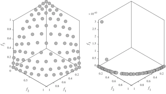
Challenge in diversity. In the process of optimizing a many-objective problem, NSGA-III may encounter a situation, that is, some reference point has no attached individual. Individuals are concentrated on certain reference points, while there has no individual in the vicinity of other reference points. Thus the algorithm cannot search for the areas near these reference points without attached individuals. NSGA-III focuses on searching for good individuals in some regions, therefore, individuals selected into next generation are from these regions. The algorithm loses its diversity to a certain degree. In extreme cases, all the individuals in a population are located in some areas, and other areas will not be searched. Let us take the DTLZ4 [41] function as an example. Fig. 2-(a) shows the evenly distribution of the optimal solutions of DTLZ4 when the population size is 100. Fig. 2-(b) shows a distribution of solutions optimized by NSGA-III. It can be seen that most areas of the solution space are not being searched. NSGA-III discards searching some areas and the distribution of the solutions is concentrated in a region like a curve. In order to overcome this challenge, a strategy needs to be considered to preserve the diversity of the population.

(a) An evenly distribution of the solutions of DTLZ4 0 0 0.2 0.4 0.2 f 3 0.6 0.4 f 2 f1 0.5 0.8 0.6 1 0.8 1 1

(b) A non-evenly distribution of solutions optimized by NSGA-III on DTLZ4 f 3 0 0.5 1 0.2 0.2 1.5 10-63 2 0.4 0.4 f₁ f₂ 2.5 0.6 0.6 3 0.8 0.8 1 1

Figure 2: The distribution of the optimal solutions on DTLZ4

Challenge in convergence. The ideal point in NSGA-III is composed of the minimum value of each objective currently obtained, but it does not correspond to a real point in the solution space, or an actual individual in a population. However, there exists a point (individual) which corresponds to the minimum value of each objective. Although this individual does not take a minimum value on other objectives, it still indicates a potential good search area. Using an individual with a minimum value on a single objective may speedup the convergence of the algorithm. An individual with a minimum value on one objective belongs to the layer

F1. In theory, all the individuals in this layer should be selected to enter the next generation. However, in many MaOPs, the number of non-dominated individuals increases sharply as the number of objectives increases. If the number of individuals inF1 exceeds the population size, then a niche selection strategy is used to select individuals for next generation. This selection strategy can not guarantee that an individual with a single objective minimum enters the next generation. Thus it is necessary to retain these individuals in a special way to guide the algorithm to converge quickly.

3. A Novel Two-archive Strategy

In this paper, a novel two-archive strategy is proposed to improve the performance of evolutionary many-objective optimization algorithms based on reference points. The two archives are uniform archive and single elite archive.

3.1. Uniform Archive Strategy

The uniform archive strategy aims to ensure that an algorithm is able to search the entire solution space, and in particular, to search an area in which no individual currently exists. This strategy keeps individuals closest to each reference point into a uniform archive. These individuals will participate in evolutionary operations with the same probability as other individuals in each generation. From the perspective of assuring population diversity, this strategy ensures that an algorithm has the ability of searching the entire solution space.

The process of implementing the strategy is described as follows: First, calculate the distance values between individuals and each reference point. Then the individual which is the closest to each reference point is added into the uniform archive. When more than one individual are at an equal distance from a certain reference point, the individual which is the closest to the ideal point is retained.

Determination of reference points. Das and Dennis’s [42] systematic approach is used to determine the set of reference pointsZ on a normalized hyper-plane. It can be formalized as Eq. 1.

Z={λ1, λ2, . . . , λH}, H = (m+p−1

p ).

(1)

Here,H is the number of reference points. λjis thejthreference point, and satisfiesλj_i ∈{0_p,1_p, . . . ,p_p}and

∑m

i=1λ j

i = 1, j= 1,2, . . . , H. mis the number of objectives of a MaOP, and each objective coordinate will

be divided intoppart. More details about the determination of reference points can be seen in [35].

Normalization. Since the values of sub-objective functions of a many-objective problem cannot be com-pared directly, themin−maxmethod is used to normalize the function values of each sub-objective. The normalization equation is described as follows:

Fi(X) = (f1i(x), f2i(x), ..., fmi (x)), fi(x) = fi(x)−Zimin Zmax i −Zimin . (2)

In the above Eq. 2,fi(x) represents the value of theithobjective, wherei= 1,2, ..., m, andmis the number

of objectives,fi(x) is the value offi(x) after normalization,Zimin is the minimum of theithobjective, and Z_imax is the maximum of the ith objective. fi

m(x) is the mth objective value of the ith individual after

normalization. Fi(x) is the fitness value of theithindividual after normalization.

Select individuals in the uniform archive. After normalization, the selection of individuals remaining to the uniform archive is formalized as Eq. 3:

uk = arg N

min

j=1||Fj(X)−Z k_||, U ={u1, u2, ...uk...uh}.

(3)

In Eq. (3), uk represents the elite individual corresponding to the kth reference point, and Fj(x) is the

individuals of thekth_{reference point. Z}k_{is thek}th_{reference point. U is the set of individuals in the uniform}

archive,his the number of reference points.

Clearly, if there are k reference points in the solution space, there are corresponding k individuals in the uniform archive. In order to maximize the diversity of a population, if an individual closest to some reference point has been placed in the uniform archive, another individual not in the uniform archive but sub-closest to the reference point will be selected to ensure there has no repetitive individual in the archive.

Algorithm of generating the uniform archive. Algorithm 1 describes the procedure of generating the uniform archive. In Algorithm 1, line 1 is used to calculate the Euclidean distance between each member ofP and each reference point ofZ, and save the distance values in matrixB. Then sortBon line and save the indexes in matrixnewB and the corresponding Euclidean distance values in matrixBdist. Awhileloop is used to determine non-repeated individuals of the uniform-archive in line 4-11. The numbers of rows and columns of newB need to be calculated for the while loop. The results of Algorithm 1 are stored in U and U d, respectively. The members of the first column of matrixnewB are the indexes of non-repeated individuals which are the closest to each reference point. They are the individuals of the uniform-archive and stored in

U. The distance values between reference points and the corresponding individuals in the uniform-archive are stored inU d.

Algorithm 1Generate-uniform-archive

Require: P: a set of individuals as population.

Z: a set of reference points on the normalized hyper-plane.

Ensure: U: a set of individuals in the uniform archive.

U d: a set of Euclidean distance values between each reference point and the corresponding individual in the uniform archive.

1: B = pdist2(Z, P) //Calculate the Euclidean distance between each member of P and each reference point ofZ. The distance values are saved in matrixB.

2: [Bdist, newB] = sort(B,2) //SortB on line and save the index in matrixnewB and the corresponding distance values in matrixBdist.

3: [Bline, Bnum]=size(newB)

//Before thewhileloop, calculate the numbers of rows and columns of newB, and store them inBline

andBnum, respectively.

4: while size(unique(newB(:,1)),1)< Blinedo

5: fori=1 toBnum−1 do

6: if ismember(newB(i+1,1),newB(1:i,1)) then

7: newB(i+ 1,1 :Bline−1) =newB(i+ 1,2 :Bline)

8: Bdist(i+ 1,1 :Bline−1) =Bdist(i+ 1,2 :Bline)

//If there has a duplicate individual, replace it by the next column one.

9: end if

10: end for

11: end while

12: U =newB(:,1)

13: U d=Bdist(:,1)

Algorithm of updating the uniform archive. During the iterative process, individuals in the uniform archive are updated constantly and participate in the evolution with the same probability as other individuals. Algorithm 2 shows how to update the uniform archive. In the process of updating the individuals in uniform archive, Algorithm 1 is used in the newly generated individuals because only the Euclidean distances between the newly generated individuals and each reference point need to be calculated. The values of the index and distance are sorted in matricesB and Bdist, respectively. Then the Euclidean distance values ofU dt

andBdistare compared. Consider the nearest individual of each reference point one by one. For theU dt+1

Algorithm 2Update-U-archive

Require: osP : a set of individuals of offspring population.

Z: a set of reference points on normalized hyper-plane.

Ut: a set of individuals in the uniform archive in the tthiteration.

U dt: a set of Euclidean distance values between each reference point and the corresponding

individual in the uniform archive in thetth_iteration.

Ensure: Ut+1;U dt+1.

1: [Bdist, B] = Generate-uniform-archive(osP, Z)

2: fori=1 to size(Z,2)do 3: if Bdist(i,1)< U dt(i)then 4: U dt+1(i) =Bdist(i,1) 5: Ut+1(i) =B(i,1) 6: else 7: U dt+1(i) =U dt(i) 8: Ut+1(i) =Ut(i) 9: end if 10: end for

the value of U dt(i), replace U dt(i) with Bdist(i,1). Ut+1(i) is also replaced by B(i,1). The individual

corresponding to the reference point in the original uniform archive will be updated.

3.2. Single Elite Archive Strategy

In NSGA-III, the ideal point is a virtual point, which is used to guide the evolution direction. Each element value of the ideal point is the smallest single objective value obtained by the current population. For example, zmin

i is the minimum value of the ith objective function obtained by the current population.

The ideal pointZideal _{= (z}min

1 , z2min, . . . zminm ) does not correspond to a real individual in the population.

Recalling particle swarm optimization (PSO), the global optimal solutiongbestand the local optimal solution pbest are kept to guiding the evolution. Inspired from PSO, the individual with the minimum value of a

single objective is kept in a single elite archive and participate in evolution to generate new individuals. These single elite individuals in the current generation can help the algorithm converge rapidly.

Select individuals in the single elite archive. The single elite archive strategy is described as follows: let

individual_ibest be the ith single elite individual corresponding to arg minzi. Retain such individuals into

the single elite archive to participate in evolution, and update them constantly. The elite individuals can help the algorithm converge rapidly. The selection of individuals that remain to the single elite archive is formalized by Eq. (4):

individual_ibest= arg minzi,

F(individualbest_i ) = (f1(arg minzi), f2(arg minzi), . . . , fm(arg minzi)).

(4)

In Eq. (4),ziis the ithelement of the ideal pointZideal,Zideal = (z1min, z2min, . . . zminm ). individualbesti is the ith_{single elite individual, andF(individual}best

i ) represents its fitness value.

Algorithm of generating the single elite archive. Algorithm 3 describes the procedure of generating the single elite archive. In Algorithm 3, the input populationP is composed by individuals whose type are defined as a structure. The objective function value of each individual is stored inP.objs. Theith_{objective minimum}

value of the current population is saved as a part of ideal pointZideal_,Zideal_{= (z}min

1 , z2min, . . . zmmin). Line 1

is used to store the minimum value of each objective function ofP inZideal_{, and returns the indices of these}

corresponding individuals inZindi. Line 2 is used to store these corresponding individuals in the single elite

Algorithm 3Generate-single-elite-archive

Require: P : a population composed of individuals.

Ensure: SEA: a set of individuals, each individual is a single elite.

Zideal: a vector named ideal point that each element value ofZ is the minimum of each objective.

1: [Zideal, Zindi] = min(P.objs,[ ],1) 2: SEA=P(Zindi)

Discussion about single elite individuals. In fact, single elite individuals are Pareto dominant solutions of the current population. They belong to the layerF1. According to the selection strategy of NSGA-III, they will be the first choice for the next generation population. If the number of individuals inF1 is less than

the population sizeN, these single elite individuals will surely be chosen to enter the next generation. But in most MaOPs, unfortunately, the number of individuals in the layer F1 is often larger than the size of

population. In this case, a niche technique is applied to selectingN individuals from F1, that is, a single

elite individual may not be selected. Thus, a single elite archive is necessarily to be used to ensure that these individuals get involved in evolutionary operations.

3.3. Proposed Algorithm: NSGA-III-UE

NSGA-III-UE is designed within the framework of NSGA-III to which the uniform archive and single elite archive are added. The uniform archive is used to keep individuals closest to each reference point for maintaining population diversity. The single elite archive is used to keep individuals with the best single objective values for fastening the algorithm convergence. Algorithm 4 describes NSGA-III-UE.

At the beginning of NSGA-III-UE, line 4 is Algorithm 1 which generates a uniform archive. Line 5 is Algorithm 3 which generates a single elite archive. They are used to determine initial individuals in the two archives. During the iteration, line 7 and line 9 allow these individuals in the two archives to participate in evolution with other individuals. Simulated two-point crossover (SBX) [43, 44] operator and polynomial variation [45]are used as same as NSGA-III’s operator. Line 10 is the process of updating the uniform archive using Algorithm 2. Only the distance values from the newly generated individuals to each reference point need to be calculated. After that, parents and descendants are merged in line 11, and sorted based on the non-dominated relationship in line 12. Then, the algorithm uses the framework of NSGA-III to select the individuals of next generation in lines 13-24. Line 25 is the updating process of the single elite archive. Single elite individuals are selected from individuals of the (t+ 1)th_generation.

3.4. Complexity Analysis of NSGA-III-UE

NSGA-III-UE is an improved version of the classical NSGA-III. Like NSGA-III, when NSGA-III-UE selects individuals into the next generation, these individuals are attached to corresponding reference points. The complexity of this process isO(M N H). For the process of selecting individuals from the layer Fl by

the niche strategy, its computational complexity is O(H). The computational complexity of determining the ideal point isO(M N).

Different from NSGA-III, NSGA-III-UE adds two extra archives. However, none of them needs to be handled in a special way. For the single elite archive, single elite individuals can be directly reserved when NSAG-III determines the Zmin, therefore, it does not require additional calculation time. For the

uniform archive strategy, individuals closest to reference points are retained no matter whether there has an individual attached to the reference point or not. Calculating the vertical distances from individuals to reference points requires O(N H) steps, and determining the closest individual for each reference point requires O(NlogH) steps. Therefore, in the worst case, NSGA-III-UE increases the computational com-plexity to max{O(N H), O(NlogH)}. Due toO(NlogH)< O(N H)< O(N2M), the overall computational complexity of NSGA-III-UE is still as same as that of NSGA-III, that is, max{O(N2 logM−2N), O(N2M)}. In fact, for most of the MaOPs, the number of individuals in the layer F1 is larger than the size of population N. NSGA-III needs to take some time to select N individuals from F1 by using the niche technique, while III-UE needs less time. Therefore, for some MaOPs, the operating time of NSGA-III-UE is less than that of NSGA-III.

Algorithm 4NSGA-III-UE

Require: H: the number of reference points.

N: the size of population.

Ensure: Pt+1. 1: t= 0

2: P0= population initialization

3: Z=Generate-Reference-Points(H)

4: [U0, U d0]= Generate-uniform-archive(P0, Z)

5: [Zideal,SEA0]=Generate-single-elite-archive(P0)

6: while termination criteria is not metdo 7: St=SEAt 8: i= 1 9: Qt=Operator(Pt, Ut) 10: [Ut+1, U dt+1]=Update-U-archive(Qt, Z, Ut, U dt) 11: Rt=Pt∪Qt 12: (F1, F2, . . .)=Non-dominated-sort(Rt) 13: while|St|< N do 14: St=St∪Fi 15: i=i+ 1 16: end while 17: Fl=Fi 18: if |St|=N then 19: Pt+1=St 20: else 21: Pt+1=∪lj−=11Fj

22: Pn=Niching(N − |St|, Z, Zmin, Fl, Pt+1) //Choose N − |St| individuals from Fl according to the

Niching selection.

23: Pt+1=Pt+1∪Pn 24: end if

25: [Zideal_,SEA

t+1]= Generate-single-elite-archive(Pt+1) //Update the single elite archive. 26: t=t+ 1

3.5. Differences from Other Algorithms

NSGA-III-UE shares a few common features with existing methods in references, such as Two-Arch2 [32] which uses two-archive strategy to balance diversity and convergence and Elite-NSGA-III [38] which uses a reference point-based strategy to maintain population diversity. However, NSGA-III-UE significantly differs from the existing methods in two aspects.

Two archives. Some algorithms [30, 32, 46, 47] adopt two-archive strategy which divides the non-dominated solution set into two archives. Although the term of two-archive in these algorithms is the same as ours, the context of two-archive is completely different from ours which means a uniform archive and a single elite archive. In [30, 32, 46, 47], one is a convergence archive (CA) which stores non-dominated solutions, while the other is a diversity archive (DA) that stores individuals not dominating any solu-tion. During the evolutions of these algorithms, individuals in two archives act as parents to generate offspring. The offspring that dominate any solution in either CA or DA are added to CA, while the offspring that dominate no solution are added to DA.

Uniform strategy: Elist-NSGA-III [38] also adopts a uniform archive strategy which is similar to ours. Both algorithms use reference points to maintain population diversity. However, the implementations are different. In Elite-NSGA-III, the individuals attached to a reference point have a chance to be taken as an elite individual and participate in evolution. If there is no individual attached to a reference point, the area near that reference point will not be searched. In our algorithm, the uniform archive strategy retains the individuals closest to each reference point, and does not abandon any search area even no individual attached to the reference point.

In addition, Elite NSGA-III selects an individual which is the closest to the origin as elite among all individuals attached to a reference point, whereas our uniform archive selects the individual closest to the reference point as elite. Our uniform archive strategy ensures the population diversity and has the ability of searching the entire solution space. Fig.3 illustrates the difference between the elite pool in Elite-NSGA-III and our proposed uniform archive method.

Figure 3: Difference between Elite-NSGA-III and NSGA-III-UE

In Elite-NSGA-III, no individual covers the direction of vector r4, and the area around r4 is hard to be searched. In NSGA-III-UE, according to the uniform archive strategy, the individual din the

tthgeneration and e′ in the (t+ 1)th generation closest to r4 are used as reserved individuals of the reference point r4. So that each reference point has an adjacent individual to be retained, and the

4. Experiments

4.1. Experimental Design

Our proposed algorithm, NSGA-III-UE, is compared with several classical and state-of-the-art algo-rithms. Experimental results are analyzed from seven perspectives for investigating the performance of NSGA-III-UE.

The first experiment is to evaluate the performance of these algorithms on WFG functions in terms of IGD, HV and operating time. The second and third experiments are used to show the performance from the perspective of test functions and objective numbers. Furthermore, the fourth experiment is designed to illustrate the efficiency of these algorithms on DTLZ functions. Then, boxplots are used to illustrate the stability of these algorithms. In the sixth experiment, variants of NSGA-III-UE are used to analyze the effect of the uniform archive and the single elite archive, respectively. Finally, the applicability of NSGA-III-UE is analyzed in the seventh experiment.

These experiments were run on Windows (Intel (R) Xeon (R) CPU [email protected], 8.00GBRAM) 64-bit operating system. Matlab2016 is used for simulation verification.

4.2. Test Functions

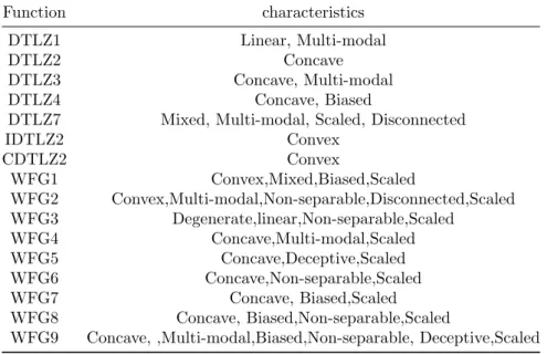
Thanks to the scalable number of objectives, Walking-Fish-Group(WFG) [48] and Deb-Thiele-Laumanns-Zitzler (DTLZ) [41] functions have become two standard test suites for testing evolutionary many-objective optimization algorithms. For DTLZ functions, only DTLZ1, DTLZ2, DTLZ3, DTLZ4, and DTLZ7 are considered because the Pareto fronts of DTLZ5 and DTLZ6 with more than 3 objectives are unknown; CDTLZ2 is a convex problem and IDTLZ2 [49] is an inverse of DTLZ2. Table 1 describes characteristics of these test functions.

Table 1: The characteristics of the test functions

Function characteristics

DTLZ1 Linear, Multi-modal

DTLZ2 Concave

DTLZ3 Concave, Multi-modal

DTLZ4 Concave, Biased

DTLZ7 Mixed, Multi-modal, Scaled, Disconnected

IDTLZ2 Convex CDTLZ2 Convex WFG1 Convex,Mixed,Biased,Scaled WFG2 Convex,Multi-modal,Non-separable,Disconnected,Scaled WFG3 Degenerate,linear,Non-separable,Scaled WFG4 Concave,Multi-modal,Scaled WFG5 Concave,Deceptive,Scaled WFG6 Concave,Non-separable,Scaled WFG7 Concave, Biased,Scaled WFG8 Concave, Biased,Non-separable,Scaled

WFG9 Concave, ,Multi-modal,Biased,Non-separable, Deceptive,Scaled

4.3. Algorithms under Comparison

The proposed algorithm NSGA-III-UE is compared with eleven state-of-the-art algorithms, listed as below:

1. NSGA-III [35] is a non-dominated sorting genetic algorithm using reference points. It solves many-objective optimization problems based on classical NSGA-II [36].

2. Two-Arch2 [32] uses two archives to focus on convergence and diversity separately, and assigns indicator-based and Pareto-based selection principles to the two archives. It is a low complexity algorithm.

3. I-DBEA [23] is a variant based on MOEA/D which uses reference direction to guide algorithm search and uses priority distance comparison mechanism. It can balance the diversity and convergence speed simultaneously.

4. EFRRR [24] is an aggregation algorithm for MaOPs. EFR uses an integrated ranking method to determine the order of individuals. Using a restriction order based on EFR, solutions of EFRRR are only allowed on sort in the corresponding weight vector which close to the part of function.

5. θ-DEA [21] is an algorithm based on a new dominance relationship that combines the fitness evaluation mechanism of MOEA/D with the diversity of NSGA-III. The ranking pattern can give consideration to both convergence and uniform distribution.

6. Elite-NSGA-III [38] is an improved NSGA-III which is similar to the algorithm that proposed in this paper. The details of the difference between Elite-NSGA-III and the proposed algorithm NSGA-III-UE can be found in Section 3.5.

7. MOEA/DD [37] is a combination of MOEA/D [12] and NSGA-III [35]. It uses hybrid mechanism of the Pareto dominance-based fitness evaluation and the MOEA/D framework. MOEA/DD can be seen as an improved version of MOEA/D which is a classical decomposition-based multiobjective optimization algorithm.

8. dMOPSO [50] combines the idea of Particle Swarm Optimization (PSO) with MOEA/D. dMOPSO uses global optimal particle to guide the search direction and re-initialized memory to ensure the diversity of the algorithm.

9. HypE [11] is a classic metric-based MOEAs. For a given MaOPs, maximizing hypervolume metric is equivalent to finding the Pareto front.

10. SPEA2SDE [28] integrates a Shift-based Density Estimation(SDE) into SPEA2 [27] in the fitness assignment and archive truncation procedures. SPEA2SDE has very competitive on the problem of DTLZs [41].

11. RVEA [14] is a reference vector-guided evolutionary algorithm that can be largely categorized into the decomposition-based approach. In RVEA, reference vectors are used to guide search process, and an angle-penalized distance is used to balance the convergence and diversity of solutions. RVEA has high efficiency in dealing with MaOPs where the functions are not well normalized.

The source code of these algorithms, except for Elite-NSGA-III, comes from Plat EMO [51].

4.4. Parameter Settings

Although parameters involved in each algorithm are not exactly the same and the complexities of the tested functions are different, the identical setting of common parameters is necessary for comparing the advantages and disadvantages of these algorithms.

The number of objectives in test functions is set tom={5,8,10,12,15}. The corresponding number of decision variables is set ton={14,17,19,21,24}, wheren=m+k−1 andkis set to 10 except IDTLZ1 in whichn={9,12,14,16,19}and DTLZ7 in whichn={24,27,29,31,34}, respectively. The identical setting of population size is 100, and the maximum times of iteration is 10000. Simulated two-point crossover (SBX) [43, 44] operator and polynomial variation [45] are used in NSGA-III, Elite-NSGA-III and θ-DEA which are based on NSGA-III, with the distribution index setting to 20. θis set to 5 inθ-DEA. MOEA/DD and I-DBEA use the aggregation function of type PBI, and the neighborhood size T is set to 10. The parameterk in EFRRR is set to 2, and the threshold Ta and weight w in dMOPSO is set to 2 and 0.4,

respectively. αis set to 2 andf ris set to 0.1 in RVEA. Each algorithm runs independently for 30 times on each test function.

4.5. Evaluation Criterion

The performance evaluation of evolutionary many-objective optimization algorithms generally includes two aspects. One is convergence, which can be measured by calculating the distances between the solutions found by an algorithm and the true Pareto solutions. The other is diversity, that is, whether the solutions found by an algorithm are uniformly distributed along the PF. In this article, IGD[7, 52], HV[53, 54], Spread[55] and Operating time are used to indicate the performance of the algorithms.

Inverted Generational Distance(IGD) is a commonly used comprehensive indicator that can evaluate convergence and diversity simultaneously. The smaller the IGD value, the better the algorithm. The formula can be described as Eq.5:

IGD(A, P∗) = ∑ x∈P∗ min y_∈Ad(x, y) |P∗| . (5) where A is an approximate solution set of the PF obtained by an algorithm, P∗ is a set of uniformly distributed sampling points of the real PF,d(x, y) is the Euclidean distance between the individualxin P∗

and the individualy inA.

Generalized Spread(IGS) is a diversity indicator. The smaller the spread, the better the distribution

diversity of the algorithm. The related formulas are described as Eq. 6:

IGS= m ∑ i=1 d(ei, A) + ∑ x∈A |d(x, A)−d| m ∑ i=1 d(ei, A) +|P∗|d , d(x, A) = min x,y∈A,y̸=x||F(x)−F(y)|| 2 , d= 1 |A| ∑ x∈A d(x, A). (6)

whered(x, A) is the Euclidean distance, the value is the Euclidean distance betweenxand the point closest toxinA. dis the average value ofd(x, A), ande1, e2, ...emaremextreme solutions inP∗.

Hypervolume(HV) is a comprehensive performance metric which is usually considered in MaOPs whose PF have not yet been known. HV calculates the volume of objective space between the obtained solution set and a reference point. The larger the HV value, the better the algorithm. In this paper, we use 106

sampling points to ensure the accuracy. The formula of HV [56] can be described as Eq. 7:

HV(fref, A) = Λ(∪[f1(y), f ref

1 ]× · · · ×[fm(y), fmref]), f_mref =max⟨Am∪fmref⟩.

(7) where A is an approximate solution set obtained by an algorithm, y is an individual in A, Am refers to

the value of the objective m in current population. fref _{is a chosen reference point, andf}ref

m refers to the

maximum value of the objective m in previous generations. Λ(.) is the Lebesuge measure[57].

Operating T imeis used to evaluate the computational complexity of an algorithm. The less the operating time, the better the algorithm.

4.6. Experimental Results and Analysis

The proposed algorithm, NSGA-III-UE, is compared with several classical and state-of-the-art algorithms in terms of IGD, HV, Spread, and Operating Time. The performance of each algorithm on WFGs and DTLZs with different objective numbers are illustrated in the following tables. The following tables show the average value of each algorithm running 30 times. In Tab. 2 and Tab. 6, the superscript of each datum is the rank for each algorithm, and the last lines show the number of times that each algorithm obtains the best value. The table-head numbers correspond to the algorithms: NSGA-III-UE (1), NSGA-III (2), Two-Arch2 (3), I-DBEA (4), EFRRR (5),θ-DEA (6), Elite-NSGA-III (7), dMOPSO (8), MOEA/DD (9), HypE (10), RVEA (11), and SPEA2SDE (12), respectively. The optimal value of each line is highlighted by gray shading.

Table 2: Average IGD values of each algorithm running 30 times on WFGs with different objective numbers

Problem M 1 2 3 4 5 6 7 8 9 10 11 12

WFG1 5 1.89e+09 1.78e+07 1.83e+08 1.74e+06 1.39e+03 1.39e+02 1.65e+04 2.16e+012 2.01e+010 2.13e+011 1.66e+05 1.37e+01 8 2.75e+05 2.71e+04 2.80e+07 2.75e+06 3.16e+010 2.97e+09 2.52e+02 3.26e+012 2.56e+03 2.93e+08 3.20e+011 2.29e+01 10 3.32e+07 3.16e+04 3.22e+05 5.72e+012 3.52e+010 3.42e+09 3.24e+06 3.91e+011 3.08e+03 3.35e+08 2.79e+01 2.85e+02 12 4.04e+010 3.77e+05 3.77e+06 4.09e+011 3.83e+08 3.81e+07 3.70e+04 4.41e+012 3.69e+03 3.87e+09 3.23e+01 3.31e+02 15 4.87e+06 4.81e+03 4.89e+07 1.42e+112 4.87e+05 4.92e+08 4.77e+02 5.61e+010 5.05e+09 4.84e+04 5.77e+011 4.30e+01 WFG2 5 7.69e-11 8.24e-12 8.57e-15 8.59e-16 8.25e-13 8.29e-14 8.66e-17 4.36e+012 4.17e+011 8.90e-18 1.40e+09 2.07e+010

8 2.36e+01 2.84e+04 2.57e+03 6.82e+010 2.56e+02 2.94e+05 3.03e+06 7.98e+011 8.89e+012 4.12e+08 3.25e+07 5.07e+09 10 5.77e+03 5.73e+02 5.06e+01 9.42e+010 6.63e+06 6.51e+05 7.06e+07 1.62e+111 1.63e+112 7.81e+08 5.87e+04 8.71e+09 12 7.60e+06 7.64e+07 7.56e+05 9.85e+09 8.17e+08 7.35e+04 6.59e+03 1.94e+111 2.04e+112 6.39e+02 5.22e+01 1.12e+110 15 8.93e+05 8.98e+06 8.06e+04 1.88e+110 7.68e+02 7.03e+01 7.85e+03 2.72e+111 2.77e+112 9.57e+07 1.00e+18 1.81e+19 WFG3 5 8.14e-18 7.67e-17 5.08e-12 8.21e-19 7.19e-15 6.63e-14 7.64e-16 9.07e-111 9.27e-112 7.41e-21 8.66e-110 5.96e-13

8 1.18e+03 1.24e+05 1.16e+02 8.84e+012 1.56e+07 1.68e+08 1.24e+04 3.00e+010 3.01e+011 1.12e-11 2.99e+09 1.42e+06 10 1.68e+03 1.99e+08 1.54e+02 1.12e+112 1.98e+07 1.90e+05 1.77e+04 5.45e+011 4.07e+010 1.61e-11 3.71e+09 1.96e+06 12 2.01e+04 2.17e+06 1.91e+02 1.34e+112 2.44e+07 1.96e+03 2.09e+05 7.77e+011 7.66e+010 2.05e-11 4.63e+09 2.75e+08 15 5.35e+05 5.50e+06 2.58e+02 1.70e+112 5.98e+08 5.33e+04 5.67e+07 1.21e+111 1.12e+110 2.50e-11 7.90e+09 4.52e+03 WFG4 5 1.35e+02 1.36e+03 1.35e+01 1.40e+07 1.49e+010 1.36e+04 1.37e+05 2.36e+012 1.47e+09 1.51e+011 1.39e+06 1.40e+08 8 3.82e+01 3.92e+05 3.85e+02 1.41e+112 4.38e+07 4.27e+06 3.91e+04 8.50e+011 4.68e+09 7.08e+010 4.43e+08 3.85e+03 10 5.63e+04 5.75e+05 5.29e+02 1.91e+112 5.62e+03 5.82e+07 5.80e+06 1.13e+111 6.26e+09 1.05e+110 6.03e+08 5.22e+01 12 6.94e+01 7.06e+06 7.03e+05 2.31e+112 6.97e+02 7.17e+07 7.00e+04 1.37e+111 7.47e+09 1.26e+110 7.38e+08 6.99e+03 15 1.18e+12 1.21e+14 1.18e+13 3.12e+112 1.55e+17 1.30e+16 1.21e+15 1.70e+19 1.61e+18 2.17e+111 1.93e+110 9.15e+01 WFG5 5 1.33e+03 1.33e+02 1.20e+01 1.37e+06 1.50e+010 1.34e+05 1.33e+04 1.65e+012 1.45e+09 1.51e+011 1.37e+07 1.40e+08 8 3.87e+01 3.95e+04 3.94e+03 1.19e+112 4.65e+09 4.23e+08 3.99e+05 6.34e+011 5.31e+010 4.09e+06 4.16e+07 3.93e+02 10 5.67e+02 5.75e+05 5.70e+03 1.93e+112 5.79e+06 5.80e+07 5.74e+04 9.33e+011 7.77e+010 7.64e+09 6.02e+08 5.17e+01 12 7.11e+02 7.16e+04 7.28e+07 2.39e+112 6.96e+01 7.20e+05 7.16e+03 1.06e+111 9.29e+09 1.03e+110 7.54e+08 7.21e+06 15 1.22e+12 1.23e+14 1.22e+13 3.10e+112 1.48e+18 1.30e+16 1.23e+15 1.50e+110 1.58e+111 1.48e+19 1.47e+17 9.72e+01 WFG6 5 1.36e+01 1.36e+03 1.36e+02 1.39e+07 1.51e+010 1.36e+04 1.36e+05 2.87e+012 1.45e+09 1.53e+011 1.38e+06 1.45e+08 8 4.01e+03 4.14e+06 4.13e+05 1.27e+112 4.49e+09 4.28e+08 4.12e+04 8.98e+011 4.61e+010 3.84e+01 4.21e+07 3.86e+02 10 5.94e+04 6.23e+06 6.03e+05 1.91e+112 5.80e+02 5.93e+03 6.34e+07 1.13e+111 7.02e+09 8.10e+010 6.54e+08 5.16e+01 12 7.27e+03 7.43e+07 7.36e+04 2.33e+112 7.13e+02 7.38e+05 7.40e+06 1.36e+111 7.70e+09 9.34e+010 7.69e+08 6.90e+01 15 1.27e+13 1.28e+14 1.06e+12 3.06e+112 1.62e+110 1.31e+16 1.30e+15 1.73e+111 1.52e+18 1.45e+17 1.53e+19 9.15e+01 WFG7 5 1.37e+03 1.37e+02 1.20e+01 1.40e+07 1.53e+011 1.38e+05 1.37e+04 2.08e+012 1.48e+09 1.50e+010 1.39e+06 1.43e+08 8 3.90e+01 4.00e+03 4.06e+05 1.17e+112 4.45e+08 4.30e+07 4.03e+04 7.04e+011 4.57e+09 4.80e+010 4.26e+06 3.95e+02 10 5.60e+02 5.73e+06 5.81e+07 1.85e+112 5.67e+03 5.81e+08 5.73e+05 9.10e+011 5.93e+09 7.40e+010 5.73e+04 5.10e+01 12 7.08e+02 7.14e+03 7.55e+09 2.27e+112 7.40e+08 7.24e+06 7.18e+04 1.14e+111 7.25e+07 1.08e+110 7.24e+05 6.75e+01 15 1.19e+14 1.20e+15 1.11e+12 3.09e+112 1.68e+110 1.29e+16 1.19e+13 1.59e+18 1.54e+17 1.80e+111 1.65e+19 8.85e+01 WFG8 5 1.37e+04 1.35e+02 1.38e+05 1.38e+06 1.47e+011 1.35e+01 1.36e+03 2.01e+012 1.46e+010 1.44e+09 1.40e+07 1.41e+08 8 3.89e+01 3.95e+02 3.99e+04 1.38e+112 4.38e+09 4.06e+06 4.00e+05 8.49e+011 4.26e+07 5.02e+010 4.35e+08 3.95e+03 10 5.83e+02 6.20e+09 6.06e+06 1.86e+112 6.00e+04 5.70e+01 6.13e+07 1.09e+111 6.05e+05 7.39e+010 6.18e+08 5.91e+03 12 7.49e+02 7.49e+03 8.21e+08 2.33e+112 8.21e+09 7.50e+04 7.56e+07 1.31e+111 7.53e+06 1.11e+110 7.52e+05 6.80e+01 15 1.24e+12 1.27e+14 1.26e+13 3.06e+112 1.57e+18 1.29e+16 1.28e+15 1.65e+19 1.67e+110 1.69e+111 1.56e+17 9.06e+01 WFG9 5 1.28e+03 1.27e+01 1.30e+05 1.32e+06 1.42e+09 1.28e+02 1.28e+04 2.73e+012 1.43e+010 1.44e+011 1.34e+08 1.33e+07 8 3.62e+01 3.66e+02 3.69e+04 1.18e+112 4.11e+08 3.97e+06 3.67e+03 7.85e+011 5.00e+09 5.86e+010 4.09e+07 3.77e+05 10 5.42e+02 5.50e+05 5.61e+07 1.93e+112 5.49e+04 5.49e+03 5.50e+06 1.01e+111 6.79e+010 6.67e+09 5.92e+08 5.15e+01 12 7.09e+04 7.11e+05 7.76e+08 2.39e+112 7.22e+06 6.94e+02 7.07e+03 1.13e+110 8.17e+09 1.18e+111 7.40e+07 6.90e+01 15 1.17e+12 1.17e+14 1.17e+15 3.10e+112 1.47e+18 1.23e+16 1.17e+13 1.50e+19 1.47e+17 1.66e+111 1.61e+110 9.23e+01

count 9 1 4 0 1 3 0 0 0 6 3 18

4.6.1. The Overall Performance on WFG Functions

The first experiment demonstrates the overall performance of twelve algorithms on WFG functions. Table 2 shows the result of IGD on 45 tests of 9 functions. In table 2, NSGA-III-UE obtains the optimal value 9 times, accounting for 20.0%. The results demonstrate NSGA-III-UE is better than most of the other algorithms, except for SPEA2SDE. HypE has the best performance on WFG3 and records 6 times for the best IGD values. Two-Arch2 produces the best results 4 times,θ-DEA and RVEA 3 times. NSGA-III and EFRRR win just once. I-DBEA, Elite-NSGA-III, dMOPSO and MOEA/DD do not return any optimal value on WFGs. As shown in Tab. 2, SPEA2SDE has 18 occurrences of the best values; therefore, more analysis should be done to explain the performance of NSGA-III-UE. Tab. 3 shows the total ranks and average ranks of all test functions of each algorithm. Form these values, we can observe the overall performance of each algorithm. The total rank of NSGA-III-UE is 145, while SPEA2SDE is 171. The overall sorting of SPEA2SDE is lower than the proposed algorithm which has an overall sorting of 1. In summary, although NSGA-III-UE does not achieve the most occurrences of optimal value on WFGs, the overall performance on IGD metric is still better than the other algorithms.

As an overall indicator, HV is used to further illustrate the performance of NSGA-III-UE. Fig. 4 shows the HV ranks of each algorithm on WFGs. The reference vector of HV is generated by taking the maximum objective values from the union of approximation sets. We can see that most of the HV ranks of NSGA-III-UE are better than, or similar to, the other algorithms. That means the performance of NSGA-III-NSGA-III-UE on HV is comparative to, and in some cases, better than, other algorithms. Tab. 4 gives the specific values of

Table 3: IGD analysis of various algorithms on WFGs

1 2 3 4 5 6 7 8 9 10 11 12

times of the best 9 1 4 0 1 3 0 0 0 6 3 18

the rate of optimal values 20.00% 2.22% 8.89% 0.00% 2.22% 6.67% 0.00% 0.00% 0.00% 13.33% 6.67% 40.00% total of ranks 145 200 188 476 303 234 208 402 492 367 324 171

average rank 3.2 4.4 4.2 10.6 6.7 5.2 4.6 8.9 10.9 8.2 7.2 3.8

overall sorting 1 4 3 11 7 6 5 10 12 9 8 2

Table 4: HV analysis of various algorithms on WFGs

1 2 3 4 5 6 7 8 9 10 11 12

times of the best 4 0 0 1 7 14 2 0 0 9 0 8

the ratio of optimal values 8.89% 0.00% 0.00% 2.22% 15.56% 31.11% 4.44% 0.00% 0.00% 20.00% 0.00% 17.78% total of ranks 252 208 375 397 219 117 148 486 328 256 375 162

average rank 5.6 4.62 8.33 8.82 4.87 2.60 3.29 10.80 7.29 5.69 8.33 3.60

overall sorting 6 4 9 11 5 1 2 12 8 7 9 3

HV rankings. The HV values of HypE must be good. Compared to the rest of the algorithms, NSGA-III-UE is better than seven algorithms and worse than SPEA2SDE, EFRRR andθ-DEA. SPEA uses a clustering technique to estimate the density of an individual, and a shift-based density estimation (SDE) can reflect the convergence of the other individuals with regard to the individual. The result of SPEA2SDE is good on both diversity and convergence but the optimization process takes more time. EFRRR uses an integrated ranking method and a restriction order to determine the order of individuals. θ-DEA uses an environmental selection mechanism namedθdominance, and combines the benefits of NSGA-III and MOEA/D. Utilizing the aggregation function-based fitness in MOEA/D,θ-DEA results in a better compromise between diversity and convergence in MaOPs. Similar to SPEA2SDE, bothθ-DEA and EFRRR have no advantage in terms of optimization time, and as Tab. 2 shows, they are not good on IGD metric.

W1 W2 W3 W4 W5 W6 W7 W8 2 4 6 8 10 12 NSGA-III-UE W1 W2 W3 W4 W5 W6 W7 W8 2 4 6 8 10 12 NSGA-III W1 W2 W3 W4 W5 W6 W7 W8 2 4 6 8 10 12 Two-Arch2 W1 W2 W3 W4 W5 W6 W7 W8 2 4 6 8 10 12 I-DBEA W1 W2 W3 W4 W5 W6 W7 W8 2 4 6 8 10 12 EFRRR W1 W2 W3 W4 W5 W6 W7 W8 2 4 6 8 10 12 W1 W2 W3 W4 W5 W6 W7 W8 2 4 6 8 10 12 Elite-NSGA-III W1 W2 W3 W4 W5 W6 W7 W8 2 4 6 8 10 12 dMOPSO W1 W2 W3 W4 W5 W6 W7 W8 2 4 6 8 10 12 MOEA/DD W1 W2 W3 W4 W5 W6 W7 W8 2 4 6 8 10 12 HypE W1 W2 W3 W4 W5 W6 W7 W8 2 4 6 8 10 12 RVEA W1 W2 W3 W4 W5 W6 W7 W8 2 4 6 8 10 12 SPEA2SDE

Figure 4: The rank of HV values of each algorithm on each function with different objective numbers

Tab. 5 gives the average operating time values of NSGA-III-UE, Elite-NSGA-III, NSGA-III, EFRRR,

θ-DEA, SPEA2SDE and HypE which have advantage on HV or IGD. The data in parentheses after average values are standard deviations. Consistent with our analysis above, NSGA-III-UE is much better than

Table 5: Average operating time values of some algorithms running 30 times on WFGs with different objective numbers

Problem M NSGA-III-UE Elite-NSGA-III NSGA-III EFRRR θ-DEA SPEA2SDE HypE WFG1 5 1.0350(8.52e-2) 1.2025 (3.88e-2) 1.6386 (1.31e-1) 1.1029 (3.88e-2) 1.0836 (1.13e-1) 24.408(5.56e-1) 50.586(1.17e+2)

8 1.1449 (1.74e-1) 1.7035 (4.41e-1) 1.9423 (2.50e-1) 1.3264 (8.14e-2) 1.4548 (3.53e-1) 27.801 (6.11e-1) 71.918(1.63e+2) 10 1.2704 (2.28e-1) 2.8580 (8.69e-1) 2.7558 (7.24e-1) 1.3819 (1.25e-1) 1.5328 (3.28e-1) 28.888 (5.68e-1) 87.741(2.04e+2) 12 1.3035 (1.74e-1) 1.8287 (4.24e-1) 2.2502 (9.62e-1) 1.2637 (4.94e-2) 1.4722 (3.40e-1) 29.869 (7.90e-1) 103.09(2.46e+2) 15 2.1405 (5.54e-1) 5.6715 (7.06e-1) 4.4708 (3.36e-1) 3.7613 (3.02e-1) 3.8211 (4.73e-1) 30.783 (6.75e-1) 162.73 (4.17e+2) WFG2 5 1.2200 (1.07e-0) 9.6806e-1 (3.56e-2) 1.5999 (2.09e-1) 1.0936 (3.34e-2) 1.0610 (9.93e-2) 26.001 (4.64e-1) 112.62 (2.64e+2) 8 1.2167 (1.09e-1) 1.9854 (3.79e-1) 2.1588 (2.70e-1) 1.2879 (4.03e-2) 1.5041 (2.02e-1) 29.556 (5.79e-1) 167.7 (3.40e+2) 10 1.5166 (2.28e-1) 2.9580 (2.17e-1) 3.0647 (4.69e-1) 1.8402 (1.34e-1) 2.2011 (3.82e-1) 30.787 (6.56e-1) 157.50e (3.64e+2) 12 1.5939 (1.68e-1) 2.2162 (8.19e-2) 2.8714 (4.00e-1) 1.8147 (1.20e-1) 2.2546 (3.38e-1) 31.696 (7.66e-1) 154.06e (3.47e+2) 15 2.4495 (7.70e-1) 5.6483 (1.80e-1) 4.4563 (3.30e-1) 3.9520 (2.33e-2) 4.0694 (4.04e-1) 32.471 (8.58e-1) 232.25 (5.80e+2) WFG3 5 1.5841 (1.66e-0) 1.5705 (2.17e-1) 1.9777 (2.62e-1) 1.1040 (3.15e-2) 1.5333 (2.53e-1) 31.619 (8.42e-1) 74.349 (1.45e+2) 8 1.6552 (2.42e-1) 3.3741 (2.35e-1) 3.3919 (1.38e-0) 2.0660 (3.52e-2) 2.8250 (6.47e-1) 32.843 (8.07e-1) 88.626 (1.78e+2) 10 1.7424 (2.45e-1) 3.5850 (2.72e-1) 3.5624 (6.45e-1) 2.2520 (2.51e-2) 2.9402 (5.28e-1) 33.272 (8.14e-1) 95.556 (1.90e+2) 12 1.7573 (1.46e-1) 2.6392 (3.90e-2) 3.0575 (5.05e-1) 1.9315 (4.77e-2) 2.5539 (4.23e-1) 33.717 (8.93e-1) 101.91 (2.04e+2) 15 2.3157 (3.19e-1) 5.4811 (7.51e-2) 4.5271 (2.88e-1) 3.9271 (2.19e-2) 4.1926 (3.21e-1) 34.110 (8.89e-1) 175.15(4.14e+2) WFG4 5 1.0352 (9.24e-2) 9.9099e-1 (5.96e-2) 1.6354 (2.96e-1) 1.0877 (3.41e-2) 1.1121 (1.46e-1) 29.044 (7.49e-1) 443.5(2.93e+1) 8 1.4613 (1.43e-0) 1.5826 (1.40e-1) 2.0419 (2.34e-1) 1.2204 (2.76e-2) 1.3246 (1.54e-1) 31.144 (8.12e-1) 570.09 (3.39e+1) 10 1.4141 (1.47e-1) 2.1024 (3.30e-1) 2.6329 (4.63e-1) 1.3424 (6.00e-2) 1.5232 (1.62e-1) 31.712 (7.58e-1) 620.98 (3.22e+1) 12 1.5484 (1.50e-1) 1.9193 (1.45e-1) 2.5486 (2.67e-1) 1.3786 (4.09e-2) 1.6358 (2.00e-1) 32.331 (8.65e-1) 674.24 (5.45e+1) 15 2.2643 (3.14e-1) 5.4074 (6.82e-2) 4.5224 (3.13e-1) 3.0513 (4.86e-1) 2.8994 (4.14e-1) 32.850 (8.83e-1) 1410.9(9.75e+1) WFG5 5 1.0058 (8.26e-2) 9.2283e-1 (2.43e-2) 1.5546 (1.48e-1) 1.0757 (2.65e-2) 1.0946 (1.45e-1) 28.657 (6.25e-1) 65.163(1.47e+2) 8 1.1388 (9.85e-2) 1.4003 (6.80e-2) 1.9199 (2.58e-1) 1.1890 (2.43e-2) 1.2528 (1.49e-1) 31.319 (7.31e-1) 93.750 (2.43e+2) 10 1.2509 (1.27e-1) 1.5899 (1.62e-1) 2.2707 (3.01e-1) 1.2842 (2.75e-2) 1.4285 (2.72e-1) 32.036 (7.72e-1) 96.550 (2.40e+2) 12 1.4965 (2.67e-1) 1.5930 (1.10e-1) 2.2857 (3.39e-1) 1.3031 (5.32e-2) 1.4576 (1.77e-1) 32.647 (7.69e-1) 113.71 (3.03e+2) 15 1.9246 (3.14e-1) 4.4984 (8.45e-1) 4.0050 (5.38e-1) 2.5733 (5.23e-1) 2.4352 (2.88e-1) 33.284 (7.77e-1) 167.96 (4.84e+2) WFG6 5 1.0021 (1.27e-1) 9.0701e-1 (2.42e-2) 1.5552 (1.43e-1) 1.0759 (3.27e-2) 1.0714 (1.46e-1) 26.051 (5.19e-1) 45.314 (1.03e+2) 8 1.1022 (6.97e-2) 1.3873 (8.94e-2) 2.2748 (1.37e-0) 1.1856 (2.19e-2) 1.2441 (1.34e-1) 28.888 (7.04e-1) 60.972(1.45e+2) 10 1.2480 (1.21e-1) 1.8853 (4.54e-1) 2.3265 (3.40e-1) 1.2805 (3.16e-2) 1.3894 (1.50e-1) 29.420 (6.60e-1) 65.016 (1.50e+2) 12 1.4435 (1.53e-1) 1.5778 (1.63e-1) 2.2858 (2.69e-1) 1.3353 (5.40e-2) 1.4157 (1.27e-1) 29.776 (5.80e-1) 75.830 (1.81e+2) 15 2.0639 (3.26e-1) 5.2170 (6.24e-1) 4.2594 (4.91e-1) 2.4231 (6.16e-1) 2.4365 (2.80e-1) 30.414 (6.92e-1) 136.02 (4.07e+2) WFG7 5 1.0406 (7.63e-2) 9.5735e-1 (3.22e-2) 1.6111 (1.46e-1) 1.0963 (3.66e-2) 1.1069 (1.09e-1) 30.434 (7.05e-1) 70.475 (1.69e+2) 8 1.1981 (1.00e-1) 1.5005 (1.17e-1) 2.0078 (2.15e-1) 1.2298 (4.04e-2) 1.3598 (1.90e-1) 31.618 (7.22e-1) 81.358 (1.90e+2) 10 1.3697 (1.49e-1) 1.9856 (3.38e-1) 2.6583 (5.33e-1) 1.3850 (3.72e-2) 1.5165 (1.70e-1) 31.713 (7.76e-1) 90.024 (2.11e+2) 12 1.8726 (1.25e-0) 2.0769 (1.35e-1) 2.8359 (3.58e-1) 1.3915 (9.31e-2) 1.6190 (2.61e-1) 31.995 (7.03e-1) 94.807 (2.22e+2) 15 2.4348 (3.18e-1) 5.4583 (9.63e-2) 4.5948 (2.73e-1) 3.3893 (7.03e-1) 3.0894 (4.75e-1) 32.421 (7.30e-1) 171.88 (5.03e+2) WFG8 5 1.0179 (9.92e-2) 9.3239e-1 (6.22e-2) 1.6048 (2.12e-1) 1.0945 (3.47e-2) 1.0752 (1.36e-1) 25.117 (4.99e-1) 43.010 (9.39e+1) 8 1.2036 (2.00e-1) 1.6679 (4.49e-1) 2.1347 (5.34e-1) 1.3299 (1.77e-1) 1.3069 (1.88e-1) 27.165 (5.23e-1) 57.981 (1.43e+2) 10 1.4148 (2.36e-1) 2.4788 (5.32e-1) 3.0074 (6.89e-1) 1.4852 (2.66e-1) 1.6779 (5.03e-1) 27.958 (5.55e-1) 65.979 (1.62e+2) 12 1.5802 (2.09e-1) 2.0142 (2.63e-1) 2.7024 (5.06e-1) 1.6310 (2.66e-1) 2.1299 (5.79e-1) 28.421 (6.09e-1) 77.617 (1.99e+2) 15 2.3701 (4.69e-1) 5.3885 (2.78e-1) 4.5610 (3.03e-1) 3.9253 (1.20e-1) 3.3503 (6.15e-1) 29.150 (6.25e-1) 141.12(4.23e+2) WFG9 5 1.0741 (1.46e-1) 9.8078e-1 (2.73e-2) 1.6260 (1.54e-1) 1.1076 (3.19e-2) 1.1353 (1.05e-1) 30.972 (1.05e+1) 599.39 (1.08e+2) 8 1.2657 (1.59e-1) 1.6426 (1.71e-1) 2.1684 (3.27e-1) 1.2877 (3.85e-2) 1.3895 (2.55e-1) 32.683 (7.71e-1) 712.85 (1.02e+2) 10 1.4568 (2.08e-1) 2.0313 (3.14e-1) 2.7478 (4.74e-1) 1.3862 (5.88e-2) 1.5750 (2.87e-1) 33.134 (8.13e-1) 797.74 (9.65e+1) 12 1.6494 (2.47e-1) 2.0247 (1.09e-1) 2.8474 (4.49e-1) 1.4026 (5.92e-2) 1.6248 (3.01e-1) 33.624 (7.43e-1) 910.99 (1.29e+2) 15 2.3916 (3.59e-1) 5.3259 (2.07e-1) 4.6353 (3.81e-1) 3.0002 (6.35e-1) 2.5791 (4.01e-1) 34.071 (9.15e-1) 1599.8 (1.86e+2)

count 28 7 0 10 0 0 0

SPEA2SDE, EFRRR andθ-DEA on the operating time metric. When the number of objectivesmis more than 5, NSGA-III-UE needs less time than NSGA-III and Elite-NSGA-III. The reason is, for most of the high-dimensional objective problems, NSGA-III-UE does not need to spend time on the niche selection. More details can be seen in Section 3.4.

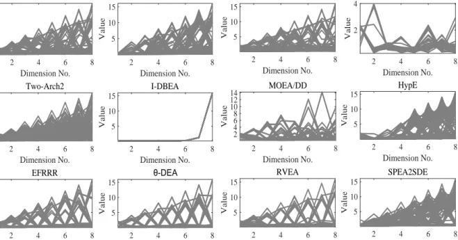
Take WFG9 with 8 objectives as an example. Fig. 5 shows the parallel coordinates plots [58] of the Pareto set obtained by the compared algorithms. The visualization results of the solution sets [59] obtained by the algorithms can further illustrate the differences of the performance .

Reviewing the results of these algorithms on IGD, HV and Operating time, it can be concluded that NSGA-III-UE has a considerable advantage over other methods on WFGs.

4.6.2. The Perspective of Test Functions

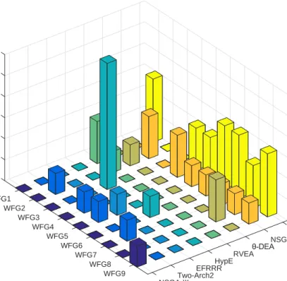
Fig. 6 analyzes the performance of eight algorithms from the perspective of test functions. Because I-DBEA, Elite-NSGA-III, dMOPSO and MOEA/DD do not get any optimal value on WFG functions with

m={5,8,10,12,15}, these four algorithms are excluded in the comparison. The histogram in Fig. 6 shows the statistical result of the remaining eight algorithms on the times of obtaining the optimal IGD values. Among these algorithms, NSGA-III-UE obtains the optimal value with 2 times on WFG2 and WFG4, corresponding to 33.33%, and one times on WFG5, WFG6, WFG7, WFG8 and WFG9. It is better than NSGA-III, Two-Arch2, EFRRR, HypE, and RVEA which only obtain once or none. NSGA-III-UE is worse than SPEA2SDE and RVEA on WFG1. On WFG3, HypE is the best algorithm which gets all the five times of the optimal value. Reviewing the above results, we can draw a conclusion that NSGA-III-UE is better than most of the algorithms on most WFG functions except WFG1 and WFG3. In Subsection 4.6.7, an analysis is provided to explain why NSGA-III-UE performs poorly on functions like WFG1 and WFG3.

2 4 6 8 Dimension No. 5 10 15 Value NSGA-III-UE 2 4 6 8 Dimension No. 5 10 15 Value NSGA-III 2 4 6 8 Dimension No. 5 10 15 Value Two-Arch2 2 4 6 8 Dimension No. 5 10 15 Value I-DBEA 2 4 6 8 Dimension No. 5 10 15 Value EFRRR 2 4 6 8 Dimension No. 5 10 15 Value 2 4 6 8 Dimension No. 5 10 15 Value Elite-NSGA-III 2 4 6 8 Dimension No. 2 4 Value dMOPSO 2 4 6 8 Dimension No. 2 4 6 8 10 12 14 Value MOEA/DD 2 4 6 8 Dimension No. 5 10 15 Value HypE 2 4 6 8 Dimension No. 5 10 15 Value SPEA2SDE 2 4 6 8 Dimension No. 5 10 15 Value RVEA

Figure 5: The parallel coordinates plots of the Pareto set obtained by each algorithm on WFG9 with 8 objectives

4.6.3. The Perspective of Objective Numbers

In this subsection, we analyze the performance of NSGA-III-UE from the view of objective

num-bers. Fig. 7 compares the ratios of optimal IGD values for all the algorithms on WFGs when m =

{3,5,8,10,12,15}. As previously mentioned, I-DBEA, dMOPSO and MOEA/DD do not return any good values on WFGs and therefore are again excluded in this comparison. From Fig. 7, it can be seen that NSGA-III-UE has a good performance when the objective number is 8, and the ratio of obtained optimal IGD value is 66.67%. Furthermore, Fig. 8 shows the IGD ranks of all the algorithms with different objective number in more detail. The numbers of the abscissa axis are the objective numbers, and the positions between each two numbers of abscissa represent the functions of WFGs. From this figure, we can observe that the ranks of our proposed algorithm are better than most of the other algorithms. Only when the objective number is 3, which is a multi-objective problem, does NSGA-III-UE fail to get the optimal value. In summary, our proposed algorithm demonstrates a significant advantage on WFGs with different objective numbers in terms of IGD, especially when the number of objectives is 8.

4.6.4. The Overall Performance on DTLZ Functions

Tab. 6 shows experimental results of eleven algorithms except SPEA2SDE which is powerful on DTLZ functions [28]. In 40 groups test of 8 functions, NSGA-III-UE gets the best average IGD value for 5 times. It is better than NSGA-III, I-DBEA, EFRRR,θ-DEA , Elite-NSGA-III, dMOPSO and RVEA, but worse than Two-Arch2, MOEA/DD and HypE. MOEA/DD has the best performance with 11 times of the best IGD value, especially on DTLZ1 and DTLZ3. HypE wins for 8 times. However, both of them do not perform well on other functions. Two-arch2 has 6 times of the best IGD value. Therefore, more analyses should be done to illustrate the performance of NSGA-III-UE.

Tab. 7 shows that the overall IGD rankings of NSGA-III-UE is 3,while Two-Arch2, MOEA/DD and HypE are 5, 8 and 6, respectively; worse than the proposed algorithm. The average ranks ofθ-DEA and Elite-NSGA-III are better than NSGA-III-UE, however, the times for obtaining the best IGD values is 2. This is lower than our algorithm which obtains 5.

0 1 2

WFG1 3

The times of the best IGD

WFG2 4 WFG3 5 6 WFG4

The best IGD times for each algorithm in each function

SPEA2SDE WFG5 _NSGA-III-UE WFG6 RVEA WFG7 HypE WFG8 EFRRR WFG9 Two-Arch2 NSGA-III

Figure 6: The times of the best IGD value of each algorithm on each function

Tab. 8. The optimization times for RVEA are consistently the smallest; however, RVEA has not achieved the optimal value on IGD. Excluding RVEA, NSGA-III-UE has the shortest optimization time in most of the tests. The operating time of NSGA-III-UE is significantly better than Two-Arch2, I-DBEA, MOEA/DD, HpyE and SPEA2SDE. Tab. 8 shows the advantage of our proposed algorithm in terms of time efficiency.

Considering the results of these algorithms on IGD and operating time, the overall performance of NSGA-III-UE is better than the other algorithms.

4.6.5. The Perspective of Stability

Boxplots Fig. 9 is used to illustrate the stability of our algorithm. The performance of NSGA-III-UE is analyzed on WFG9 with different objective numbers: m={5,8,10,12,15,20}. The compared algorithms run 30 times on each objective number. The IGD values are plotted on boxplots. The abscissa values correspond to these algorithms: NSGA-III-UE(1), NSGA-III(2), Two-Arch2(3), I-DBEA(4), EFRRR(5),

θ-DEA(6), Elite-NSGA-III(7), dMOPSO(8), MOEA/DD(9), HypE(10), RVEA(11) and SPEA2SDE(12),

respectively.

It can be seen from Fig. 9 that for WFG9, the overall IGD value distribution of NSGA-III-UE is more evenly than other algorithms. Especially, whenm={5,8,10}, the IGD values obtained by NSGA-III-UE have no outliers. When the number of objectives is 8, the datum is distributed evenly and the value is the minimum. The boxplots indicate that the performance of NSGA-III-UE is stability.