Kent Academic Repository
Full text document (pdf)
Copyright & reuse
Content in the Kent Academic Repository is made available for research purposes. Unless otherwise stated all content is protected by copyright and in the absence of an open licence (eg Creative Commons), permissions for further reuse of content should be sought from the publisher, author or other copyright holder.
Versions of research
The version in the Kent Academic Repository may differ from the final published version.
Users are advised to check http://kar.kent.ac.uk for the status of the paper. Users should always cite the published version of record.
Enquiries
For any further enquiries regarding the licence status of this document, please contact:
If you believe this document infringes copyright then please contact the KAR admin team with the take-down information provided at http://kar.kent.ac.uk/contact.html
Citation for published version
Cui, XW and Yan, Yong and Guo, M and Mu, YH and Han, XJ (2016) Localization of Continuous
Gas Leaks from a Flat-Surface Structure Using an Acoustic Emission Sensor Array. In: IEEE
International Instrumentation and Measurement Technology Conference (I2MTC 2016), 23-26
May 2016, Taipei, Taiwan.
DOI
https://doi.org/10.1109/I2MTC.2016.7520457
Link to record in KAR
http://kar.kent.ac.uk/55768/
Document Version
Localization of Continuous Gas Leaks from a
Flat-Surface Structure Using an Acoustic Emission
Sensor Array
Xiwang Cui
1,2, *Yong Yan
1,2, Miao Guo
1, Yonghui Hu
1, Xiaojuan Han
11 School of Control and Computer Engineering, North China
Electric Power University, Beijing 102206, China
2 School of Engineering and Digital Arts, University of Kent,
Kent CT2 7NT, U.K. Email: [email protected]
Abstract—Leak localization is of great importance for
pressurized vessels for reasons of safety and maintenance. This paper presents an experimental study using an Acoustic Emission sensor array coupled with a hyperbolic positioning algorithm for continuous leak localization. The study aims to detect continuous CO2 leak from an isotropic flat-surface
structure on a pressurized vessel in the Carbon Capture and Storage system. The proposed approach consists of four main stages. In the first stage, empirical mode decomposition is deployed to extract the useful signal from the noise. The second step is concerned with the estimation of the time differences of the sensor array in conjunction with correlation signal processing. The third stage estimates the distance difference between the sensing elements from the measured time differences and wave speed. Finally, a hyperbolic positioning algorithm is used to locate the leak source on the flat-surface structure. Results obtained from experiments on a 100 cm × 100 cm stainless plate demonstrate that the mean full-scale error in the leak localization is 4.9%.
Keywords—continuous leak; localization; circular sensor array; acoustic emission; hyperbolic positioning; cross correlation
1.INTRODUCTION
Pressurized vessels and containers are widely used in a range of industries. For instance, in the carbon capture and storage (CCS) process, pressurized vessels are used to store the captured CO2. It is imperative to identify and locate any
accidental leak quickly from flat-surface structures in a pressurized vessel when it occurs. Acoustic Emission (AE) technology is a promising approach to locate the leak source and has evoked much interest in recent years [1-3]. A number of sensor array configurations have been proposed in previous studies to localize the leaks from flat-surface structures [4]. Gangadharan et al. [5] proposed a sensor array of four piezoelectric sensors which were arranged in the four corners of the plate. Bian et al. [6] developed an L-type array to achieve a high accuracy on an aluminum alloy plate. Niri et al. [7] proposed an AE source localization model based on a sparse array with multiple piezoelectric sensors. It is well known that, for a large flat-surface structure, the resolution of AE localization will increase with the number of sensors and so does the computational power.
This paper proposes a new sensor array using only four AE sensors arranged in a circle for continuous leak localization on a flat-surface structure. The configuration is specific to locate a
continuous CO2 leak from an isotropic flat-surface structure in
the CCS system. Meanwhile, the proposed method incorporates algorithms of empirical mode decomposition, cross correlation and hyperbolic positioning. There have been no reported studies of this method with a small number of sensors for the intended industrial applications. The advantages of this method along with experimental results are presented and discussed.
II.METHODOLOGY
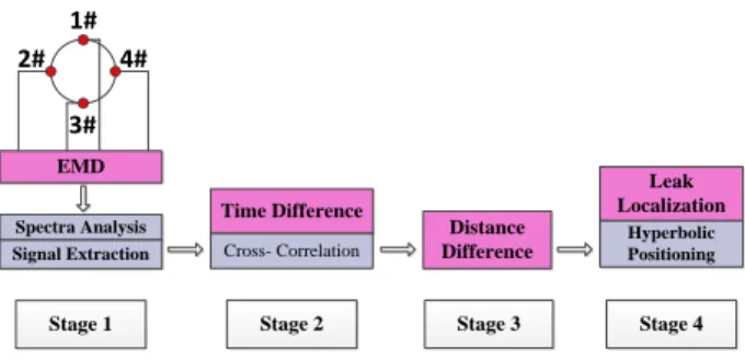
A. Sensing arrangement and leak localization
In this study the sensing elements in the AE sensor array are arranged evenly in a circle, as shown in Fig. 1. In comparison with previous studies, this new sensing arrangement has advantages of compact layout and similar attenuations and dispersions between the different sensors in the array, which is beneficial to the correlation signal analysis. The implementation of the proposed approach consists of four main stages, as illustrated in Fig. 1. In the first stage, empirical mode decomposition (EMD) is deployed to extract the useful signal from the original leak signal. In the second stage the time differences between the signals from the sensors are estimated through cross correlation. The third stage determines the distance differences between the sensors with reference to the leak source from the measured time differences and the measured AE wave speed. Finally, a hyperbolic positioning algorithm is used to locate the leak source.
EMD Spectra Analysis Signal Extraction Time Difference Distance Difference Leak Localization Hyperbolic Positioning 1# 2# 4# 3# Cross- Correlation
Stage 1 Stage 2 Stage 3 Stage 4
Fig. 1. Block diagram of the proposed approach.
B. Leak localization
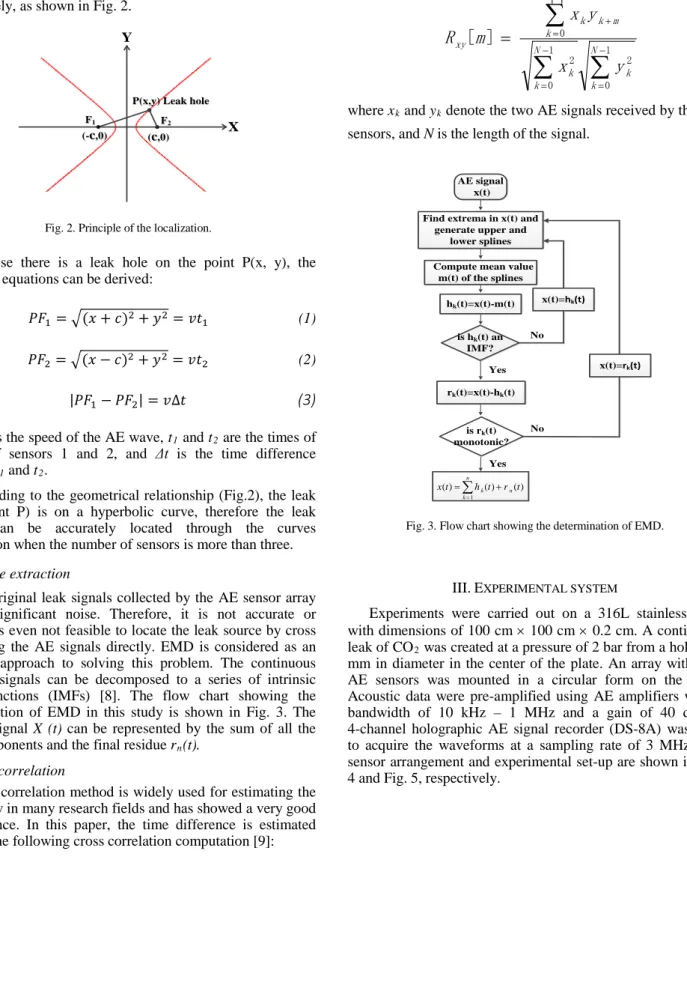
Assuming two AE sensors are installed at any positions on the plate, then a coordinate system can be established where the midpoint of these two sensors is the origin, and the connecting line of these two sensors is the horizontal axis, thus
the coordinates of sensors 1 and 2 are (-c, 0) and (c, 0), respectively, as shown in Fig. 2.
X Y
P(x,y) Leak hole P(x,y) Leak hole
(-c,0)
(-c,0) ((cc,0) ,0) F1
F1 FF22
Fig. 2. Principle of the localization.
Suppose there is a leak hole on the point P(x, y), the following equations can be derived:
= ( + ) + = (1)
= ( ) + = (2) | | =
(3)
where v is the speed of the AE wave, t1 and t2 are the times of arrival of sensors 1 and 2, and t is the time difference between t1 and t2.
According to the geometrical relationship (Fig.2), the leak hole (point P) is on a hyperbolic curve, therefore the leak source can be accurately located through the curves intersection when the number of sensors is more than three.
C. Feature extraction
The original leak signals collected by the AE sensor array contain significant noise. Therefore, it is not accurate or sometimes even not feasible to locate the leak source by cross correlating the AE signals directly. EMD is considered as an effective approach to solving this problem. The continuous leak AE signals can be decomposed to a series of intrinsic mode functions (IMFs) [8]. The flow chart showing the determination of EMD in this study is shown in Fig. 3. The original signal X (t) can be represented by the sum of all the IMF components and the final residue rn(t).
D. Cross correlation
Cross correlation method is widely used for estimating the time delay in many research fields and has showed a very good performance. In this paper, the time difference is estimated through the following cross correlation computation [9]:
∑
∑
∑
− = − = − − = +=
1 0 2 1 0 2 1 0]
[
N k k N k k m N k m k k xyy
x
y
x
m
R
(4)where xk and yk denote the two AE signals received by the two sensors, and N is the length of the signal.
Compute mean value m(t) of the splines
AE signal x(t)
Find extrema in x(t) and generate upper and
lower splines is hk(t) an IMF? hk(t)=x(t)-m(t) rk(t)=x(t)-hk(t) is rk(t) monotonic? Yes Yes No No 1 ( ) ( ) ( ) n k n k x t h t r t = =∑ + x(t)=hk(t) x(t)=rk(t)
Fig. 3. Flow chart showing the determination of EMD.
III.EXPERIMENTAL SYSTEM
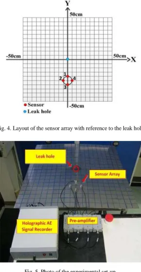
Experiments were carried out on a 316L stainless plate with dimensions of 100 cm × 100 cm × 0.2 cm. A continuous leak of CO2 was created at a pressure of 2 bar from a hole of 2
mm in diameter in the center of the plate. An array with four AE sensors was mounted in a circular form on the plate. Acoustic data were pre-amplified using AE amplifiers with a bandwidth of 10 kHz – 1 MHz and a gain of 40 dB. A 4-channel holographic AE signal recorder (DS-8A) was used to acquire the waveforms at a sampling rate of 3 MHz. The sensor arrangement and experimental set-up are shown in Fig. 4 and Fig. 5, respectively.
Fig. 4. Layout of the sensor array with reference to the leak hole.
Fig. 5. Photo of the experimental set-up.
IV.EXPERIMENTAL RESULTS AND DISCUSSION
A. Signal characteristics
The signals from the four sensors are of very similar characteristics due to the fact that they are mounted close to each other and used to detect the same leak source. Take the signal from sensor 1 as an example, the time domain waveform and corresponding frequency spectrum are plotted in Fig. 6.
It can be seen from Fig.6 that the leak signal is continuous in the time domain and has a wide spectral range of 10 kHz to 300 kHz. The signal contains frequency components in three main regions, one in the high frequency band (150 kHz – 200 kHz), the other two in the low frequency band (10 kHz – 50 kHz). Since the high frequency region is not adversely affected by the common ambient noise, the signal in this region is utilized for the localization of the leak source in this study.
(a) Time domain signal waveform.
(b) Frequency spectrum.
Fig. 6. Time domain signal waveform from sensor 1and the corresponding frequency spectrum.
Fig. 7 shows the EMD decomposition results of the original signal from sensor 1 using the method illustrated in Fig. 3. It can be seen that seven IMF components are generated. IMF1 has the highest frequency components and other IMF components have the lower frequency components. According to the above analysis, IMF1 is extracted to identify the location of the leak source.
(a) Decomposed time domain signal waveforms.
0 0.1 0.2 0.3 0.4 0.5 0.6 0.7 0.8 0.9 1 -0.2 -0.1 0 0.1 0.2 0.3 Time (ms) A m pl it ude ( v ) 0 50 100 150 200 250 300 0 5 10 15 20 Frequency (kHz) A m pl itude 0 0.05 0.1 0.15 0.2 0.25 0.3 -0.05 0 0.05 IM F 1 0 0.05 0.1 0.15 0.2 0.25 0.3 -0.05 0 0.05 IM F 2 0 0.05 0.1 0.15 0.2 0.25 0.3 -0.050 0.05 IM F 3 0 0.05 0.1 0.15 0.2 0.25 0.3 -0.05 0 0.05 IM F 4 0 0.05 0.1 0.15 0.2 0.25 0.3 -0.05 0 0.05 IM F 5 0 0.05 0.1 0.15 0.2 0.25 0.3 -0.050 0.05 IM F 6 0 0.05 0.1 0.15 0.2 0.25 0.3 -0.05 0 0.05 IM F 7 Time (ms)
(b) Frequency spectra. Fig. 7. EMD results of the leak signal.
B. Leak localization result and error analysis
The time differences between any pair of signals from the sensor array can be calculated through cross correlation. The sensor array contains four sensing elements, therefore there is a set of six cross-correlation results. If the speed of the AE signal is known, the distance difference can be calculated and then the leak source located. The speed is found to be 4610 m/s, which was measured by the Nielsen-Hsu Pencil Lead Break Test [10]. Table 1 shows one of the best measured time difference and distance difference between the signal pairs.
TABLE I. MEASURED TIME DIFFERENCES AND ERRORS
AE Sensors Time Difference (µs) Distance Difference (cm) Actual Distance Difference (cm) Absolute Error (cm) 1&2 12.33 5.69 5.50 0.19 1&3 21.67 9.99 10.00 0.01 1&4 12.0 5.53 5.50 0.03 2&3 9.67 4.46 4.50 0.04 2&4 0.33 0.15 0.00 0.15 3&4 9.67 4.46 4.50 0.04
It can be seen from Table I that the error in the determination of the distance difference is no greater than 0.2 cm. This result shows the potential advantages of the AE sensor array arranged in a circle:
(1) Degrees of attenuation and dispersion from the different sensors in the array are similar. The reason for this is that the sensors in the circular arrangement are close to each other. This advantage is beneficial to the correlation signal analysis.
(2) The maximum distance difference from leak hole to different sensors is the diameter of the circle. In this case the
two sensors (sensors 1 and 3) are located on the same line as the leak hole, as shown in Fig. 4. For all the other cases, the distance difference is smaller than the diameter of the circle. This limit is used as a threshold to judge the correlation results.
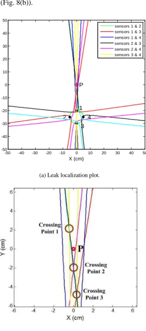
The leak localization result using the hyperbolic positioning algorithm is shown in Fig. 8. The crossing points of all hyperbolic curves are seen in the zoomed-in version of the plot (Fig. 8(b)).
(a) Leak localization plot.
(b) Zoomed-in version of (a) around the leak hole. Fig. 8. Leak localization result.
In theory, all curves should intersect at one point (i.e. the leak hole); however, in practice there are more than one crossing points due to errors in measurement. It can be seen from Fig. 8(b) that three crossing points formed by at least three curves and their coordinates are (-0.44 cm, 1.97 cm), (0.04 cm, -1.97 cm), and (0.36 cm, -4.94 cm), respectively. The location of the leak hole is thus estimated using the following equation: 0 50 100 150 200 250 300 0 5 10 IM F 1 0 50 100 150 200 250 300 0 5 10 IM F 2 0 50 100 150 200 250 300 0 5 10 IM F 3 0 50 100 150 200 250 300 0 5 10 IM F 4 0 50 100 150 200 250 300 0 5 10 IM F 5 0 50 100 150 200 250 300 0 5 10 IM F 6 0 50 100 150 200 250 300 0 5 10 IM F 7 Frequency (kHz) X (cm) Y ( c m ) P 1 2 3 4 -50 -40 -30 -20 -10 0 10 20 30 40 50 -50 -40 -30 -20 -10 0 10 20 30 40 50 sensors 1 & 2 sensors 1 & 3 sensors 1 & 4 sensors 2 & 3 sensors 2 & 4 sensors 3 & 4
( , ) = [ , + ( , ) + ( , )] (5)
The resulting coordinate of the leak hole is (-0.01 cm, -1.65 cm). The absolute error in this localization is no greater than 0.2 cm on the 100 cm × 100 cm plate. To assess the location performance of the method, the experiments were repeated for five times. Results are plotted in Fig. 9. As shown in Fig. 9, the five estimated leak locations are all below X-axis, because the actual hole is nearest to sensor 1 and many crossing points are generated near this sensor. In summary, the mean absolute error is 4.9 cm and the mean full-scale error is 4.9% (The full-scale error is defined as the absolute error normalized to the full length of the square plate).
Fig. 9. Localization error.
It must be noted that the time difference measurement is crucial in the whole localization process and even a small error can corrupt the source localization result. The time difference calculated through cross correlation usually contains several peak values. Errors will be introduced if the wrong peak is selected. More stable and accurate algorithms should be sought in the near future.
V.CONCLUSIONS
In this paper experimental investigations have been carried out using an AE sensor array arranged in a circle for continuous leak localization on a flat-surface structure. The AE signals have been decomposed using the empirical mode decomposition technique. The high frequency band of the signal (IMF1) has been used to predict the location of the leak hole through cross correlation. A total of six hyperbolic curves are generated, resulting in three crossing points formed by at least three curves. Advantages of the proposed AE sensor array have been investigated. The mean absolute error in the localization experiments on 100 cm × 100 cm plate is 4.9 cm, which is equivalent to a mean full-scale error of 4.9%.
ACKNOWLEDGEMENT
The authors wish to acknowledge the Chinese Ministry of Science and Technology and the Chinese Ministry of Education for providing financial support for this research as part of the 111 Talent Introduction Projects (B13009) at North China Electric Power University. This work was also
supported by the Fundamental Research Funds for the Central Universities (No. 2014XS40). Xiwang Cui would like to thank the China Scholarship Council for offering an academic exchange grant for his visit to the University of Kent.
REFERENCES
[1] A. Mostafapour and S. Davoudi, “Analysis of leakage in high pressure pipe using acoustic emission method,” Applied Acoustics, vol. 74, no. 3, pp. 335-342, 2013.
[2] P. Bestagini, M. Compagnoni, F. Antonacci, A. Sarti, and S. Tubaro, “TDOA-based acoustic source localization in the space–range reference frame,” Multidimensional Systems and Signal Processing, vol. 25, no. 2, pp. 337-359, 2014.
[3] P. Murvay and I. Silea, “A survey on gas leak detection and localization techniques,” Journal of Loss Prevention in the Process Industries, vol. 25, no. 6, pp. 966-973, 2012.
[4] B. Yoo, A. S. Purekar, Y. Zhang, and D. J. Pines,
“Piezoelectric-paint-based two-dimensional phased sensor arrays for structural health monitoring of thin panels,” Smart Materials and Structures, vol. 19, no. 7, 075017, 2010.
[5] R. Gangadharan, G. Prasanna G, M. R. Bhat, C. R. Murthy, and S. Gopalakrishnan, “Acoustic emission source location and damage detection in a metallic structure using a graph-theory-based geodesic approach,” Smart materials and structures, vol. 18, no. 11, 115022, 2009. [6] X. Bian, Y. Zhang, Y. Li, X. Gong, and S. Jin, “A new method of using
sensor arrays for gas leakage location based on correlation of the time-space domain of continuous ultrasound,” Sensor, vol.15, no. 4, pp. 8266-8283, 2015.
[7] E. D. Niri, A. Farhidzadeh, and A, S. Salamone, “Nonlinear Kalman Filtering for acoustic emission source localization in anisotropic panels,” Ultrasonics, vol. 54, no. 2, pp.486-501,2014.
[8] B. Liu, S. Riemenschneider, and Y. Xu. “Gearbox fault diagnosis using empirical mode decomposition and Hilbert spectrum,” Mechanical Systems and Signal Processing, vol. 20, no. 3, pp. 718-734,2006. [9] X. Qian and Y. Yan, “ Flow measurement of biomass and blended
biomass fuels in pneumatic conveying pipelines using electrostatic sensor-arrays,” IEEE Transactions on Instrumentation and Measurement, vol. 61, no. 5, pp. 1343–1352, 2012.
[10] W. H. Prosser, K. E. Jackson, S. Kellas, B. T. Smith, J. Mckeon, and A. Friedman, “Advanced waveform-based acoustic emission detection of matrix cracking in composites,” Materials Evaluation, vol. 9, no. 9, pp. 1052-1058, 1995.