CONSISTENCY OF SEMI-SUPERVISED LEARNING
ALGORITHMS ON GRAPHS: PROBIT AND ONE-HOT METHODS FRANCA HOFFMANN , BAMDAD HOSSEINI , ZHI REN , AND ANDREW M. STUART ∗
Abstract. Graph-based semi-supervised learning is the problem of propagating labels from a small number of labelled data points to a larger set of unlabelled data. This paper is concerned with the consistency of optimization-based techniques for such problems, in the limit where the labels have small noise and the underlying unlabelled data is well clustered. We study graph-based probit for binary classification, and a natural generalization of this method to multi-class classification using one-hot encoding. The resulting objective function to be optimized comprises the sum of a quadratic form defined through a rational function of the graph Laplacian, involving only the unlabelled data, and a fidelity term involving only the labelled data. The consistency analysis sheds light on the choice of the rational function defining the optimization.
Key words. Semi-supervised learning, classification, consistency, graph Laplacian, probit, spec-tral analysis.
AMS subject classifications. 62H30, 68T10, 68Q87, 91C20.
1. Introduction. Semi-supervised learning (SSL) is the problem of labelling all the points in a dataset, by leveraging correlations and geometric information in the data points, together with explicit knowledge of a subset of noisily observed labels. The primary goal of this article is to analyze the probit and one-hot methods for transductive SSL. We elaborate conditions under which both of these methods con-sistently recover the correct labels of the dataset when the label noise is small and the unlabelled data is clustered, in a sense that we make precise. The formulation and analysis demonstrates how ideas from unsupervised learning and, in particular spec-tral clustering, can be used as prior information; this prior information is enhanced, or sets up a competition with, labelled data. In so doing, our analysis also elucidates the role of parameter choices made when setting up the balance between labelled and unlabelled data. Furthermore, we exhibit useful properties of the probit and one-hot methods, including a representer theorem for the classifier, and a natural dimension reduction which follows from this theorem and is impactful in practice.
1.1. Background And Literature Review. We start by giving informal state-ments of the problem to be solved, and a brief literature review. Consider a set of nodesZ= {1,⋯, N}and an associated set offeature vectorsX= {x1, x2,⋯, xN}. Each feature vectorxjis assumed to be a point inRd. X may thus be viewed as a function
X ∶ Z ↦ Rd or as an element of
Rd×N. We refer to X as unlabelled data. Suppose there exists a function l ∶ Z ↦ {1,2,⋯, M} that assigns one of M distinct labels to each point in Z. That is, for every point j ∈Z the value l(j) =m indicates thatj
belongs to classm or islabelledas m. Throughout this article we assume that every point inZ belongs to one class only.
Now let Z′⊆Z be a subset of the nodes with ∣Z′∣ =J ≤N and define y∶ Z′↦
{1,2,⋯, M}to be anoisily observed labelof each point inZ′. We refer toyaslabelled data. With this setup we may define the SSL problem.
Problem 1.1 (Semi-Supervised Learning). Suppose Z, Z′, X and y are known.
Findl∶Z↦ {1,2,⋯, M}. ◇
∗Computing and Mathematical Sciences, Caltech, Pasadena, CA ([email protected], [email protected],[email protected],[email protected]).
1
In order to solve this problem, which is highly ill-posed, it is necessary to introduce some form of regularity on the labels, guided by the correlations in X for example, and to make assumptions about the errors in the labels provided. One approach, which we study here, is to assume that the labels onZ are defined through a latent variableu∶Z↦RM, whose regularity is defined through the unlabelled dataX, and a functionS∶RM ↦ {1,2,⋯, M}. Specifically we assume that there is a ground truth functionu†∶Z↦RM for which
(1.1) y(j) ∶=S(u†(j) +η(j)), j∈Z′,
where η(j)iid∼ ψ and ψ is the Lebesgue density of a zero-mean random variable on RM. We may now introduce the following relaxation of the SSL problem.
Problem 1.2 (Relaxed Semi-Supervised Learning). Suppose Z, Z′, X and y are known, together with the functionS and the densityψ. Findu∶Z↦RM and define
l=S○u∶Z↦ {1,2,⋯, M}. ◇
In Problem 1.3 below we will define a class of optimization functionals for u, giving an explicit instantiation of Problem1.2, and focus on the resulting optimization problems in our analysis. Before doing so we give a literature review explaining the context for this optimization approach.
The consistency of classification methods in the setting of supervised learning is well-developed; see [36] for a literature review and results applying to both binary and multi-class classification, as well as the preceding work in [33, 34, 41] which establishes the problem in the framework of Vapnik [37]. The paper [42] discusses the robustness of such supervised classification methods, allowing for a small fraction of adversarially labelled data points. There has been some recent analysis of logistic regression, and the reader may access the literature on this subject via the recent papers [11, 35]. All of this work on supervised classification focuses on the large data/large number of features setting, and often starts from assumptions that the unlabelled data is linearly separated. None of it leverages the power of graph-based techniques to extract geometric information in large unlabelled data sets. To make the connection to graph-based techniques we need to discuss unsupervised graph-based learning [3, 38]. This is a subject that has seen significant analysis in relation to consistency. The papers [31, 32] perform a careful analysis of the spectral gaps of graph Laplacians resulting from clustered data, studying recursive methods for multi-class clustering. The paper [23] introduced a way of thinking about, and analyzing, multi-class unsupervised learning based on perturbing a perfectly clustered case; we will leverage similar ideas in our work on SSL. The paper [39] introduced the idea of studying the consistency of spectral clustering in the limit of large i.i.d. data sets in which the graph Laplacian converges to a limiting integral operator; and the work [17, 18] has taken this further by working with localizing weight functions designed so that the limit of the graph Laplacian is a differential operator.
SSL is a methodology which combines the methods of unsupervised learning and of supervised classification. According to the definition in [22] “SSL can be catego-rized into two somewhat different settings, namely inductive and transductive learning
. . . inductive SSL attempts to predict the labels on unseen future data, while trans-ductive SSL attempts to predict the labels on unlabeled instances taken from the training set.” In this paper our focus is on transductive SSL. Initial attempts to solve the SSL problem employed combinatorial algorithms [9], based on an explicit math-ematical formulation stemming from Problem1.1. Zhu and collaborators introduced
a relaxation similar to Problem 1.2, leading to the influential papers [43,44]. Their approach is most easily described in the binary case in which they assumeS∶R↦R is the identity function and the labels are given in the form ±1. From a modeling viewpoint this approach is unnatural because the categorical data is assumed to also lie in the real-valued space of the latent variable. Bertozzi and Flenner [7] introduced an interesting relaxation of this assumption, by means of a Ginzburg-Landau penalty term which favours real-values close to±1 but does not enforce the categorical values ±1 exactly. The probit approach to classification, described in the classic text on Gaussian process regression [25], does not make the unnatural modeling assumption underlying Zhu’s work; instead it is based on takingS to be the sign function. How-ever the basic form of probit in [25] does not use unlabelled data to extend labels outside the labelled data set, but instead does so through regular Gaussian process regression: inductive SSL.
The extension of the probit method to graph-based transductive SSL is described in [8], where both Bayesian and optimization-based formulations are described; in that paper, (1.1) is also generalized to the level set form
(1.2) y(j) ∶=S(u†(j)) +η(j), j∈Z′,
and a Bayesian formulation of the Ginzburg-Landau relaxation of [7] is introduced. The close relationship between level set and probit formulations is discussed in [16]. The work of Belkin [2,3,5] demonstrates how both Gaussian process regression and graph-based SSL can be used simultaneously; in the sense of the definition in [22], transductive and inductive SSL are combined. All of the approaches which followed from the work of Zhu are readily generalized from the binary case to the multi-class setting, using the idea of one-hot encoding, explained in detail in subsection 3.1, in which each label is identified with a standard unit basis vector inRM.
A large number of approaches to SSL have been developed in the literature and a detailed discussion of all of them is outside the scope of this article. We refer the reader to the review articles [45] and [22] for, respectively, the state-of-the-art in 2005 and a more recent appraisal of the field that categorizes various inductive and transductive approaches to SSL and semi-supervised regression. The idea of regularization by graph Laplacians for SSL was developed in different contexts such as manifold regularization [5], Tikhonov regularization [2] and local learning regularization [40]. However, while graph regularization methods are widely applied in practice the rigorous analysis of their properties, and in particular asymptotic consistency, is not well-developed within the context of SSL. Indeed, to the best of our knowledge the consistency analysis of the probit and one-hot methods has not been tackled before. SSL may be viewed as a method for boosting, refining or questioning unsupervised graph-based learning, through labelling information; our analysis sheds light on this process.
There has been other analysis of SSL methods, not concerning consistency. In [16] the authors studied the large data and zero noise limits of the probit method. They derive a continuum inverse problem using the methodology of [17,18] that char-acterizes SSL when the number of vertices of the graph and the number of observed labels is fixed, or goes to infinity in a manner insuring a fixed fraction of labels. The authors also study the zero noise limit of probit and level-set methods for SSL and show that both problems approach the same limit as the noise variance goes to zero. In forthcoming papers [21,20] we will build on this body of work to study consistency of graph-based SSL in the limit of large unlabelled data sets.
1.2. Problem Setup And Preliminaries. Our focus in this paper is on the analysis of algorithms built from the introduction of real-(vector)-valued latent func-tions, leading to precise mathematical formulations of Problem 1.2. To make ac-tionable algorithms we need to specify precisely how the unlabelled dataX and the labelled datay are used. The approach we study here is to define the desired latent variableuas the minimizer of a function comprised of two terms, one of which enforces correlations and geometric information in the unlabelled dataX, and the other which enforces consistency with the label data y, on the assumption that they are related touas in (1.1). To this end we viewX as a point cloud inRd and associate a weight matrixW = (wij)to tuples(xi, xj)inX×X. The weightswij, which are assumed to be non-negative, are chosen to measure affinities betweenxi andxj. Since similarity between data points is a symmetric relationship, we assumewij=wjiso thatW is a symmetric matrix and define a proximity graphG= {X, W}with verticesXand edge weightsW. FromW we will construct a covariance operatorCon spaces of functions
H = {u∶Z ↦RM}, using a graph Laplacian implied by W. We also define a misfit function Φ(⋅;⋅ ) ∶H× {1,⋯, M}J ↦
Rwhich encodes the assumption (1.1) about the relationship between the labels and the latent function. With these objects we then formulate the SSL problem as a regularized optimization problem.
Problem 1.3 (Relaxed Semi-Supervised Learning As Optimization). Suppose
Z, Z′, X and y are known, together with the function S, the covariance operator C
and the misfit Φ. Find the functionu∗ defined by
(1.3) u∗=arg min u∈H 1 2⟨u, C −1u⟩ H+Φ(u;y). ◇ This optimization problem may be viewed as the MAP estimator associated to the Bayesian inverse problem of finding the distribution of u∣y when the prior onu
is a Gaussian random measure on H with covariance C and Φ(u;y)is the negative log-likelihood ofy conditioned onu, i.e.
(1.4) P(y∣u) ∝exp(−Φ(u;y)), assuming y(j) =S(u(j) +η(j)).
We refer to Φ as thelikelihood potential.
1.3. Main Contributions. The key question at the heart of this article is to identify conditions under which the minimizeru∗ of Problem1.3correctly identifies the labels. To this end, we define the following notion of consistency.
Definition 1.4 (SSL asymptotic consistency).We say that Problem1.3is
asymp-totically consistent if, for all j∈Z,
S(u∗(j))ÐÐ→a.s. S(u†(j)), as std(η(j)) ↓0, whereu† is the latent variable underlying the labelled data (1.1).
In the above and throughout the rest of the articleÐÐ→a.s. denotes almost sure (a.s.) convergence with respect to a common probability space on which the measurement noise η(j) are defined (see subsections 2.6 and 3.5 for a formal discussion of this mode of convergence). We primarily focus on the probit and one-hot methods for SSL, corresponding to specific choices of the functionS. As mentioned earlier probit is an optimization approach for binary classification that formulates Problem1.3with
M =2. The one-hot method is a generalization of probit for multi-class classification whenM ≥2. We outline these methods in detail in sections 2 and3. We show that probit and one-hot methods are asymptotically consistent in the case where the graph
Gis nearly-separable in the following sense.
Definition 1.5 (Nearly-separable graph). A weighted graph G = {X, W} is
nearly-separable into K clusters if there exist connected components Gk = {Xk, Wk}
for k∈ {1,⋯, K} so that the edges within each Gk are O(1), but the edges between
elements in differentGk areO()for a small parameter >0. In other words, up to
a reordering of the index setZ, the matrixW is nearly block diagonal.
Working in such a setting is a natural way of representing nearly clustered data, and was exploited in the paper [23] concerning unsupervised learning. The number of clusters K is an inherent geometric property of the unlabelled data X; determining a suitable choice of K in practice can be challenging and depends on the scale one is interested in. In the following informal statement of our main result we assume that each componentGk is associated with at least one pre-assigned label. The result shows that ifGis nearly separable and the ground truth functionu†assigns the same label to all points within each component Gk then the probit and one-hot methods are asymptotically consistent for an appropriate choice of matrixCso long as at least one label is observed in each componentGk. Below,Ldenotes thegraph Laplacian, a discrete diffusion operator acting on functions defined on the graphG, see Section2.3 for a precise definition.
Theorem 1.6 (Consistency of probit and one-hot). SupposeGis nearly separa-ble and letL be a graph Laplacian on G. Define the matrix C=τ2α(L+τ2I)−α with parameters τ2, α>0. AssumeS(u†)is constant on the components G
k and at least
one label is observed in each componentGk. Then the probit and one-hot formulations
are asymptotically consistent for any sequence(, τ,std(η)) ↓0along which=o(τ2). We note that is a property of the data, whilst τ is a parameter which can be determined by the user of the algorithms. Interestingly we give theory and numerical evidence showing that when =Θ(τ2)consistency may be lost. Formal statement and proof of the preceding main theorem is given in Theorem 2.15 (together with Corollaries2.14and2.16) for the probit method and in Theorem3.11(together with Corollary 3.12) for the one-hot method. An important conclusion of the theory and numerical experiments is that careful choice of parameterτis crucial for effective SSL. The take-home message here is that the use of hierarchical Bayesian methods, which tuneτautomatically to the data, can be beneficial; practical experience demonstrates this benefit [12]. A number of existing methods circumvent the issue of choosing τ
by setting it to zero and working orthogonal to the null-space of L. This forces a particular structure on the latent function uwhich may not be compatible with the data, and so we avoid such an approach. In particular, working orthogonal to the null-space ofL forces the functionuto assign a different label to at least one of the clusters. This constraint is inconsistent when the data is made up of multiple clusters that belong to the same class.
As a secondary result to the above theorem we identify a natural dimension reduction for probit and one-hot optimization problems. More precisely, we show that findingu∗ ∈H = {u∶Z ↦RM} is equivalent to a similar optimization problem for a functionb∗∈H′= {b∶Z′↦RM}. Thus we can reduce the size of the optimization problems fromN×M toJ×M. This result, which is a discrete representer theorem, has significant practical consequences whenJ ≪N.
Theorem 1.7 (Dimension reduction for probit and one-hot). The problem of
finding u∗ is equivalent to an optimization problem of the form b∗∶=arg min b∈H′ 1 2⟨b,(C ′)−1b⟩ H′+Φ′(b;y),
where C′ is a submatrix of C after restriction of rows and columns to Z′, and Φ′ is defined from Φ.
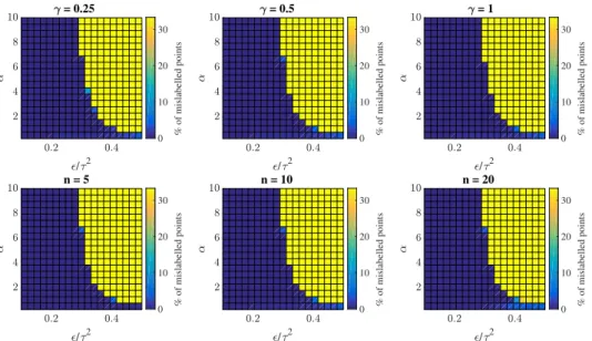
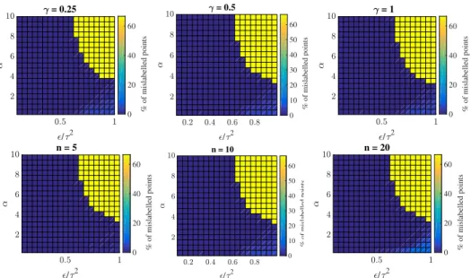
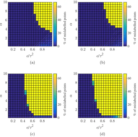
Finally we perform numerical experiments to illustrate the behavior of probit and one-hot methods beyond the theoretical setting. In particular we demonstrate that when=Θ(τ2)these methods are not always consistent. An interesting observation we make is a sharp phase transition in the accuracy of both methods. More precisely, we observe a curve in the(/τ2, α)-plane across which the probit and one-hot methods transition rapidly from being consistent into inconsistent solutions based on majority label propagation, i.e., labelling all points in the dataset according to the label that is observed most often (see Figures4.2and4.8). Intuitively this happens because, for larger values of/τ2, it is cheaper to minimize the quadratic regularization term in the optimization problem of Theorem1.7than to minimize the misfit term Φ.
1.4. Outline. Section2is devoted to analysis of the probit method whereM =2. The problem is formulated as inference for a latent real-valued function on the nodes of a graph, with the sign determining the assignation of a binary label. An optimization approach is employed in which the graph Laplacian constructed from the unlabelled data is used for regularization, and a generic zero-mean log-concave label measurement noise is assumed; this results in a convex data misfit term. We study the properties of this optimization problem, showing that the related optimization functional is convex. We prove a representer theorem and then study asymptotic consistency of the method in Corollary2.14, Theorem 2.15and Corollary 2.16, the precise statements of Theorem1.6in the probit case.
Section3has the same structure as section2but focuses on the multi-class setting (i.e., M ≥ 2) and employs the one-hot method to link a real-vector-valued latent variable to the labels. The key results here are Corollary 3.10, Theorem 3.11 and Corollary 3.12, the precise versions of Theorem 1.6 in case of the one-hot method. Section4 contains numerical experiments confirming the key theoretical results from the two preceding sections, and illustrates the behavior of probit and one-hot methods beyond the theoretical setting. In section5we summarize and discuss future work.
1.5. Notation. Throughout we useZ to denote the nodes of a graph carrying a pre-assigned unlabelled data point at each node, andZ′the subset of nodes which also carry a label. We useuto denote real-(vector)-valued functions onZ which are acted upon by a nonlinear classifier to assign labels. We use∣ ⋅ ∣to denote the cardinality of a set;⟨⋅,⋅ ⟩,∥⋅∥denote the Euclidean inner-product and norm unless stated otherwise. We employ the standard Θ, O and o notations as in [15]: given positive functions
f(s), g(s), we write
● f(s) =Θ(g(s)) if there exist constantsc1, c2, s0>0 so that 0≤c1g(s) ≤f(s) ≤c2g(s) ∀s∈ (0, s0], ● f(s) = O(g(s))if there existsc, s0>0 so that
0≤f(s) ≤cg(s) ∀s∈ (0, s0],
● f() =o(g())if for any constantc>0 there existss0(c) >0 so that 0≤f(s) <cg(s) ∀s∈ (0, s0(c)].
2. Binary Classification: The Probit Method. In subsection 2.1 we set up the probit methodology, noting that the binary classification problem (M = 2) can be formulated using a latent variable function which isRM−1−valued rather than RM−valued. In subsection 2.2we study the likelihood contribution to the optimiza-tion problem, resulting from the labelled data, and in subsecoptimiza-tion 2.3 the quadratic regularization resulting from the unlabelled data. In subsection2.4we study the pro-bit minimization problem, formulating the results via a discrete representer theorem, and in subsection2.5we study the properties of the representers via the properties of the eigenstructure of the covariance, exploiting the nearly separable graph structure. subsection 2.6 concludes the analysis of the probit method, studying consistency in some detail.
2.1. Set-Up. We start with the case of binary classification where the nodesZ
belong to only two classes. For simplicity we assume thatl(j) ∈ {−1,+1}for allj∈Z
rather than taking l(j) ∈ {1,2}. This assumption is at odds with our notation in subsection 1.2but allows for a simpler formulation of Problem1.3. Since the classes are identified with the integers+1 and−1 a natural choice for the classifier function
S is the sign function:
(2.1) S∶R↦ {−1,+1}, S(t) =sgn(t) ∶= {+1, ift≥0,
−1, ift<0.
With the above choice for S we can take the latent variable u to be a real valued function on Z, i.e.,u∶Z ↦R. We can then naturally identify the function uwith a vector u∈RN where u= (u
1, u2,⋯, uN)T and uj =u(j) forj ∈Z. This allows to view Problems 1.2 and 1.3 as the inverse problem of finding a vector u∗ in RN. In the remainder of this section we will utilize this vector notation for convenience.
2.2. The Probit Likelihood. Let us begin by deriving the likelihood potential Φ(u;y)for the probit method. LetS be as in (2.1) and recall (1.1), then
y(j) =sgn(uj+ηj), ηj iid
∼ ψ, j∈Z,
wherein we have identified the noiseη with a vectorηηη= (η1, . . . , ηN)T ∈RN. Suppose
ψ is a symmetric probability density function on R and denote the the cumulative distribution function (CDF) ofψby Ψ. Then,
P(y(j) = +1∣uj) =P(−uj≤ηj) =P(−ujy(j) ≤ηj) =Ψ(ujy(j)).
For more details on this calculation, see similar arguments for the multi-class case in Section3.2. Similarly,
P(y(j) = −1∣uj) =P(−uj>ηj) =P(ujy(j) >ηj) =Ψ(ujy(j)). From (1.4) it follows that theprobit likelihoodpotential Φ(u;y)has the form
(2.2) Φ(u;y) = − ∑
j∈Z′
log Ψ(ujy(j)).
2.3. Quadratic Regularization Via Graph Laplacians (Binary Case).
Let us now formulate a quadratic regularization term for the probit method. Recall our encoding of the nodesZ and their similarities via a weighted graphG= {X, W}
with vertices atxj and edge weightswij=wjifori, j∈Z. We denote bydi the degree of each nodei∈Z as
di∶= ∑ j∈Z
wij,
and further define the diagonal matrixD∶=diag(di) ∈RN×N. Finally, given constants
p, q∈Rwe define the graph Laplacian operator onG (2.3) L∶=D−p(D−W)D−q∈RN×N.
Different choices ofpandqresult in different normalizations of the graph Laplacian, see [4, 13, 14, 16, 17, 18, 28, 29, 38, 39] and the references therein. For example,
p=q=0 leads to the usualunnormalizedgraph Laplacian, whenp=q=1/2 we obtain thesymmetric normalizedgraph Laplacian, andp=1 andq=0 gives therandom walk
graph Laplacian. Different normalizations of the graph Laplacian have been used for spectral clustering in the literature, but a thorough understanding of the advantages and disadvantages of certain parameter choices is still lacking, see [38]. Throughout we enforcep=q in order to makeL symmetric with respect to the Euclidean inner-product, making no other assumptions regarding the value ofp, q; however our results can be generalized to p ≠ q by using appropriate D−weighted inner-products. For
p=q, we can then write for any vectorx∈RN,
(2.4) ⟨x, Lx⟩ =1 2 N ∑ i,j=1 wij∣ xi dpi − xj dpj∣ 2 .
Given a graph LaplacianLand parametersα, τ2>0 we define a family of covariance operators
(2.5) Cτ=τ2α(L+τ2I)−α∈RN×N,
where I∈RN×N denotes the identity matrix. We then use this covariance matrix to define the quadratic regularization term in Problem1.3. To this end note that in the binary case we may identifyH =RN; we make this identification in what follows in this section, and⟨⋅,⋅ ⟩then denotes the standard Euclidean inner-product.
Remark 2.1. We use the term covariance operator to refer to the matrixCτ fol-lowing the connection between optimization problems of the form (1.3) and MAP estimators within the Bayesian formulation of probit given in [8]. In the Bayesian perspective Cτ is the covariance operator of a Gaussian prior measure onu, andu∗
coincides with the MAP estimator ofu†. ◇
2.4. Properties Of The Probit Minimizer. With the likelihood Φ and co-variance matrixCτ identified we can now discuss properties of theprobit functional
(2.6) J(u) ∶=1 2⟨u, C −1 τ u⟩ +Φ(u;y), u∈R N. 8
Remark 2.2. In the following we will study the problem of minimizing J. We highlight that there are related formulations of probit which simply take a covariance
C=L−1 and consider the functional
(2.7) J(u) ∶= 1
2⟨u, Lu⟩ +Φ(u;y), u∈E, where E = {u ∈ RN ∶ ⟨u, Dp
01⟩ = 0}, 1 ∈ R
N denotes the vector of ones and Dp 01 lies in the null-space of L. We will further discuss the differences between the two
approaches in section5. ◇
Our first task is to prove existence and uniqueness of the minimizers ofJby prov-ing it is strictly convex. The followprov-ing proposition follows directly from [1, Thm. 1] and states that the CDF of a log-concave probability distribution function (PDF) is also log-concave.
Proposition 2.3 (Convexity of the likelihood potential Φ). Let ψbe a contin-uously differentiable, symmetric and strictly log-concave PDF with full support onR.
ThenΨis also strictly log-concave and so Φ(⋅;y) ∶RN ↦
Ris strictly convex. Convexity of the quadratic regularization term in (2.6) follows directly from Lemma A.1 that establishes that the matrix Cτ is strictly positive-definite when-everτ2, α>0. With the convexity of both terms in the definition ofJestablished we can now characterize its minimizer.
Proposition 2.4 (Representer theorem for the probit functional). Let G = {X, W} be a weighted graph and let ψ be a PDF that is continuously differentiable, symmetric and strictly log-concave with full support on R. Suppose the likelihood
potential Φ is given by (2.2) and the matrix Cτ is given by (2.5) with parameters
τ2, α>0. Then the following hold.
(i) The probit functional J has a unique minimizeru∗∈RN.
(ii) The minimizer u∗ satisfies the Euler-Lagrange (EL) equations
(2.8) Cτ−1u∗= ∑
j∈Z′
Fj(u∗j)ej,
where Fj(s) ∶= y(j)ψ(sy(j))/Ψ(sy(j)) and ej is the j-th standard coordinate
vector inRN.
(iii) The minimizer u∗ has a sparse representation
(2.9) u∗= ∑
j∈Z′
˜
ajcj,
where Cτej =∶ cj = (c1j,⋯, cN j)T are a subset of the column space of Cτ = (cij)i,j∈Z anda˜j∈R.
(iv) The vectoru∗defined in (2.9)solves(2.8)if and only if the coefficients˜ajsatisfy
the non-linear system of equations
˜
aj=Fj( ∑ k∈Z′
˜
akcjk), ∀j∈Z′.
Proof. (i) Since Ψ is the CDF of a random variable onRwith full support then Ψ(s) ∈ (0,1). Thus, −log Ψ ≥0 and so Φ is bounded from below. Furthermore, Φ is convex following Proposition 2.3. On the other hand, the matrixCτ−1 is strictly positive definite following LemmaA.1and so the quadratic term12⟨w, Cτ−1w⟩is strictly
convex and positive. Thus, since the functional J is bounded from below and is the sum of strictly convex functions thenJis strictly convex and has a unique minimizer. (ii) SinceψisC1(R)the CDF Ψ isC2(R)andψ/Ψ isC1(R)and locally bounded since ψ has full support. Then J ∶ RN ↦ R is differentiable and the minimizer u∗ satisfies the first order optimality condition ∇J(u∗) =0. The statement now follows by directly computing the gradient ofJ(u)with respect to u.
(iii–iv) Multiply (2.8) byCτ to get
u∗= ∑ j∈Z′ Fj(u∗j)Cτej= ∑ j∈Z′ ˜ ajcj,
where we set ˜aj = Fj(u∗j) for j ∈ Z′. Now substitute the expansion of u∗ into the definition of ˜aj to get (2.10) ˜aj=Fj⎛ ⎝( ∑k∈Z′ ˜ akck) j ⎞ ⎠,
This establishes the “only if” statement in (iv). In order to establish the converse, suppose the ˜ajsatisfy (2.10). Multiply this equation byck and sum overj∈Z′to get
∑ j∈Z′ ˜ ajcj= ∑ j∈Z′ Fj( ∑ k∈Z′ ˜ ajcjk)cj. now defineu∗= ∑j∈Z′˜ajcj to get
u∗= ∑
j∈Z′
Fj(u∗j)cj. The claim follows by multiplying this equation byCτ−1.
Remark 2.5 (Connection to kernel regression). We note that Proposition 2.4 is closely related to the representer theorem in Gaussian process and kernel regression [25, Sec. 6.2]. A particularly similar result to ours can be found in [30, Thm. 1] and
[27]. ◇
Part (iv) of Proposition2.4suggests that the problem of minimizingJis analogous to a low-dimensional optimization problem. To this end we now define a one-to-one reordering
(2.11) π∶Z′↦ {1,2,⋯, J}, π−1∶ {1,2,⋯, J} ↦Z′,
that allows us to associate the coefficients{˜aj}j∈Z′ with a vectora= (a1,⋯aJ)T ∈RJ
via
aπ(j)=˜aj, j∈Z′, and define submatrixC′∈RJ×J by the identity
(2.12) (Cτ′)π(i),π(j)=c′ij, i, j∈Z′.
That is, Cτ′ is the matrix Cτ with the rows and columns of the indices in Z∖Z′ removed. Finally, we defineb∶=Cτ′a. We then have the following natural dimension reduction for the probit optimization problem.
Corollary 2.6 (Probit dimension reduction). Suppose the conditions of
Propo-sition 2.4are satisfied. Then the following hold.
(i) The problem of finding the minimizer u∗∈RN of the functionalJ is equivalent
to the problem of finding the vectorb∗∈RJ that solves
(2.13) (Cτ′)−
1
b∗=F′(b∗), where the mapF′∶RJ↦
RJ is defined as
F′(v) = (f1(v1),⋯, fJ(vJ))T, fk(vk) ∶=Fπ−1(k)(vk).
(ii) Moreover, the vectorb∗ solves the optimization problem b∗=arg min v∈RJ J′(v), where J′(b) ∶=1 2⟨b,(C ′ τ)− 1b⟩ +Φ′(b;y), and Φ′(b;y) = − J ∑ j=1 log Ψ(bjy(π−1(j))).
(iii) The two solutions b∗∈RJ andu∗∈
RN satisfy the relationship
(2.14) u∗= ∑ j∈Z′ ((Cτ′)−1b∗) π(j)cj, and b∗k=u∗π−1(k), k= {1,2,⋯, J}.
Proof. This result follows from Proposition2.4 and direct computations.
Remark 2.7 (Variable Elimination And Gaussian Process Regression). There is a simple explanation for the finite dimensional representer theorem which underlies Proposition2.4and Proposition2.6. If we re-order the variables inuinto components
u+inZ′andu−inZ∖Z′, and re-order the components of the precision matrixP=C−1 τ then setting the gradient of Jto 0 in this re-ordered set of variables gives equations of the form ( PP++−+ PP+−−− ) ( u + u− ) = ( g(u+) 0 ).
This follows from the fact that Φ(u)does not depend on u−; the termg(u+)results from the gradient of Φ(u)with respect tou+.From this re-ordering of the equations several things are apparent: (i) the bottom row provides a linear mapping fromu+
to u− since P−− is invertible whenever Cτ is; (ii) using this linear mapping it is possible to obtain a closed nonlinear equation for u+ only, from the top row, and the linear part of this equation has a Schur complement form; (iii) the unknownu−
is recovered by solving a linear equation; (iv) the nonlinear equation foru+ may be viewed as the equation for a critical point of a functional of u+ only. These four
points are encapsulated in the previous two theorems, where they are rendered in a form familiar from Gaussian process regression and representer theorems [25]. Ideas analogous to those described in this remark underlie all representer theorems, but are not so transparent in the infinite-dimensional setting. We present the results in the abstract form of Proposition2.4and Proposition2.6to highlight the formal analogies with our companion papers [20, 21] which study the limiting optimization problems that arise when the elements of X are drawn i.i.d. at random from a probability
measure, andN → ∞,building on [18]. ◇
The expansion (2.9) indicates that the minimizer u∗ ∈ span{cj}j∈Z′; we refer
to the cj as representers. In other words, the minimizer u∗ belongs to a subspace of the column space of the covariance matrix Cτ. Recall that by definition Cτ =
τ2α(L+τ2I)−αand so we can compute the vectorsc
j by solving the linear equations, (2.15) (L+τ2I)αcj=τ2αej, j∈Z′,
that costJ linear solves involving anN×N matrix. With the {cj}j∈Z′ at hand we
can extract the matrixCτ′ and solve the nonlinear system (2.13) forb∗ and in turn compute the solution u∗ by (2.14). Then whenever J ≪ N solving the dimension reduced problem (2.13) is typically much faster than solving the full nonlinear system (2.8). We present evidence of this improved efficiency in subsection4.3in the context of the one-hot method for multi-class classification.
We now proceed to exploit the geometry in the problem dictated by the nearly-separable graph structure that forms the basic assumption underlining our consistency analysis. It is clear that the geometry ofu∗is dictated by the geometry of the vectors
cj. It is then natural for us to try to identify the geometry of thecj. By LemmaA.2 we have the expansion
(2.16) cj= N ∑ k=1 1 λk( φ φ φk)jφφφk,
where {λk, φφφk} are the eigenpairs of Cτ−1. Therefore, by analyzing the spectrum of
Cτ we can identify the geometry of the vectors cj which together with the vector
b∗ allow us to identify the minimizer u∗ and eventually prove consistency of the probit minimizer. Spectral analysis ofCτ is outlined in AppendixA, and in the next subsection we present the main propositions and assumptions that are used in the remainder of the article.
2.5. Perturbation Theory For Covariance Operators. Consider a graph
G0 = {X, W0} consisting of K < N connected components Gk, i.e., the subgraphs
Gk are connected but there exist no edges between pairs of componentsGi,Gk with
i ≠ k. Without loss of generality assume the nodes in Z are ordered so that Z =
{Z1, Z2,⋯, ZK} and theZk collect the nodes in the k-th subgraphGk. We refer to theZk as clusters. Thus, the weight matrixW0= (w(
0)
ij )satisfies
(2.17) ⎧⎪⎪⎨⎪⎪ ⎩
w(ij0)≥0 ifi≠j andi, j∈Zk for somek,
w(ij0)=0 ifi=j ori∈Zk, j∈Z`, fork≠`.
We will show that when τ is small the geometry of cj is dominated by indicator functions of the clustersZk. First, let us collect some assumptions on the graphG0.
Assumption 1. The graph G0 = {X, W0} satisfies the following conditions with
K<N:
(a) The weight matrix W0 satisfies (2.17) and has a block diagonal form W0 = diag(W˜1,⋯,W˜K)where ˜Wk are the weight matrices associated to the subgraphs
Gk.
(b) Let ˜Lk be the graph Laplacian matrices of the subgraphsGk, i.e., ˜
Lk∶=D˜k−p(D˜k−W˜k)D˜k−p
with ˜Dk denoting the degree matrix of ˜Wk. There exists a uniform constantθ>0 so that forj=1,⋯, K the submatrices ˜Lj have a uniform spectral gap, i.e., (2.18) ⟨x,L˜jx⟩ ≥θ⟨x,x⟩,
for all vectorsx∈RNk andxD˜p
k1k where 1k∈RNk are vectors of ones.
Note that the preceding assumption means that the clusters Gk are pathwise connected. Further, condition (2.18) excludes the possibility of outliers, that is, nodes of zero degree. This means that the inner product as expressed in (2.4) is well defined. In the following and throughout the remainder of the article we introduce the following notation: We define the graph Laplacian in terms of the weight matrix W0 and the associated degree matrixD0∶=diag(d(
0) i ):
(2.19) L0∶=D−0p(D0−W0)D0−p∈R N×N.
LetZ= {Z1, Z2,⋯, ZK}and define the weighted indicator functions (2.20) (χχχk)j∶=⎧⎪⎪⎨⎪⎪ ⎩ (d(j0))p, ifj∈Zk, 0, otherwise, and χχχ¯k∶= 1 ∥χχχk∥ χ χ χk.
Similarly, the weighted indicator function on the full label set is denoted by (2.21) χχχ∶=Dp01, and χχχ¯∶= 1
∥χχχ∥χχχ.
The next proposition, whose proof is given in appendixA.1, identifies the geometry of the covariance matrix constructed fromL0. The key take away is that, for small
τ, the covariance matrix is nearly block diagonal and there is negligible correlation outside clusters.
Proposition 2.8. Let G0= {X, W0} satisfy Assumption1and letL0 be a graph
Laplacian of form (2.19) on G0 and define the covariance matrix Cτ,0 on G0 for
τ2, α>0 (2.22) Cτ,0∶=τ2α(L0+τ2I)−α. Then asτ↓0, ∥cj,0− (χχχ¯k)jχχχ¯k∥ 2 ≤Ξτ4α ∀j∈Zk, wherecj,0= (c( 0) 1j ,⋯, c (0) N j) T is thej-th column ofC
τ,0, andΞ>0is a uniform constant. Thus, whenτ2αis small the vectorscj,0have a similar geometry to the set func-tions ¯χχχk. We now show that this result remains true when the graphG0is perturbed.
Consider a perturbation of the matrixW0 by modifying some of the entriesw( 0) ij and possibly making the graph connected. More precisely, letG= {X, W}where
(2.23) W=W0+
∞
∑ h=1
hWh.
We need to collect some assumptions on the perturbed matrixWto restrict the type of perturbations that are allowed.
Assumption 2. The graphG= {X, W}satisfies the following assumptions: (a) The weight matrixW satisfies expansion (2.23) withW0 satisfying (2.17). (b) The sequence of matrix norms satisfies {∥Wh∥2}h∈Z ∈ `∞, and for each h ∈ Z,
Wh= (w( h)
ij )is self-adjoint and satisfies
(2.24) {w(ijh)≥0, if wij(0)=0 for i, j∈Z, i≠j,
Note thatwij(h) may be negative for indicesi, j such thatw(ij0)>0.
Associated to the weight matrixW is a graph Laplacian and covariance matrix (2.25) L∶=D−p(D−W)D−p, Cτ,∶=τ2α(L+τ2I)−α,
whereτ2, α>0 and p∈
R. We then have the following result stating that if=o(τ2), then the geometry of the column space ofCτ, remains close to the set functionsχχχk, whilst if=Θ(τ2)then prior correlation between clusters is introduced. The proof is given in appendixA.2.
Proposition 2.9. SupposeG0 satisfies Assumption 1 andG satisfies
Assump-tion 2. For τ2, α> 0 define the covariance matrix C
τ, as in (2.25) and denote the
j-th column ofCτ, bycj,= (c( ) 1j,⋯, c () N j) T. Then
(a) If=o(τ2), then there exists a constantΞ>0independent of andτ so that ∥cj,− (χχχ¯k)jχχχ¯k∥
2
≤Ξ(2/τ4+τ4α+2), ∀j∈Zk.
.
(b) If /τ2=β >0 is constant, then there exist constants Ξ,Ξ′>0, independent of andτ so that
∥cj,− [(1−β˜)(χχχ¯)jχχχ¯+β˜(χχχ¯k)jχχχ¯k]∥ 2
≤Ξ(2+τ4α), ∀j∈Zk,
and whereβ˜= (1+Ξ′β)−α.
2.6. Consistency Of The Probit Method. Throughout this section we con-sider a graphG0= {X, W0}consisting ofKcomponents, along with perturbed graphs
G= {X, W}as introduced in the previous subsection. As before, we use Z′⊂Z to denote the set of points where labels are observed and assume the usual ordering
Z = Z1∪Z2∪ ⋯ ∪ZK where Zk denotes the k-th cluster in Z. Recall the probit assumption on the labelled data, namely that
(2.26) y(j) =sgn(u†j+ηj), j∈Z′,
where u† = (u†1,⋯, u†N)T is the vector isomorphic to the ground truth function u†. The additive noisesηj are assumed to be a rescaling of a sequence of i.i.d. samples from a reference densityψ. That is, for allj∈Z′,
(2.27) ηj=γη˜j, η˜j
iid ∼ ψ, 14
where ψ is the PDF of a centred random variable with unit standard deviation, and thus γ > 0 is the standard deviation of the ηj. Thus the ηj are i.i.d and have distribution (2.28) ψγ(t) = 1 γψ( t γ).
We recall a useful result stating that log-concave random variables have exponen-tial tails [10, Thm. 4.3.7].
Lemma 2.10. Let ψ(t) be a log-concave PDF on R. Then there is ωc > 0 such
that, for allω∈ [0, ωc),∫Rexp(ω∣t∣)ψ(t)dt< +∞.
With this lemma we can estimate the probability of the event where the observed labelsy(j)have the same value as sgn(u†j), i.e., the event where the data is exact.
Lemma 2.11. Let ψ(t) be a log-concave PDF on R. Then there exist constants
ω1, ω2>0 depending only onψ, so that P(y(j) =sgn(u†j), for allj∈Z ′) ≥ ∏ j∈Z′ [1−ω2exp(− ω1 γ ∣u † j∣)].
That is, whenγ>0 is small the data y is exact with high probability.
Proof. By Lemma2.10there exists a sufficiently smallω1>0 and constantω2>0 so that forγ>0,
ω2= ∫ R
exp(ω1
γ ∣t∣)ψγ(t)dt< +∞.
Letηj∼ψγ then by Markov’s inequality for θ>0
P(ηj≥θ) ≤ω2exp(− ω1 γ θ). Buty(j) ≠sgn(u†(j))whenever ηj< −∣u†j∣ if u†j≥0, ηj≥ ∣u†j∣ if u†j<0.
The result now follows from the symmetry of theψγ and independence of theηj. Lemma 2.12. Suppose (2.26) and (2.27) hold, ψ is log-concave and ∣u†j∣ >θ >0
for all j ∈ Z′. Then for any sequence γ ↓ 0, y(j)ÐÐ→a.s. sgn(u†j) a.s. with respect to
∏j∈Z′ψ(tj)the law of the i.i.d. sequence{η˜j}j∈z′.
Proof. Sinceψis log-concave it has exponential tails by Lemma2.10and∣η˜∣ < ∞ a.s. 1 Recall that value ofηj=γη˜j. Then for any fixed ˜ηj∈ (−∞,∞), ifγ<θ/∣η˜∣then
y(j) =sgn(u†j). Since ˜ηj are a.s. finite the result follows. Now consider a probit likelihood potential of the form
(2.29) Φγ(u;y) ∶= ∑
j∈Z′
−log Ψγ(ujy(j)), 1In fact the proof reveals that all we need is that the ˜η
jare a.s. finite, for which log-concavity
suffices.
where
(2.30) Ψγ(s) = ∫
s
−∞ψγ(t)dt, s∈R.
For, τ2, γ>0 we study the consistency of minimizers of the functionals (2.31) Jτ,,γ(u) ∶=
1 2⟨u, C
−1
τ,u⟩ +Φγ(u;y), u∈RN.
This functional is of the same form as (2.6), and so the results in section2.4apply.
2.6.1. Probit Consistency With A Single Observed Label. We start with the simple case of a single observed label. Without loss of generality assumeZ′= {1}, that is the observed label is the first point in the first clusterZ1 andu†1>0.
Proposition 2.13. Consider the single observation setting above and suppose Assumptions 1and 2 are satisfied by G0 and G. Let u∗ denote the minimizer of
Jτ,,γ and letγ>0. (a) If=o(τ2)asτ→0 then∃τ 0>0 so that∀(τ, γ) ∈ (0, τ0) × (0,∞)and∀j∈Z1 (2.32) P(sgn(u∗j) = +1) ≥1−ω2exp(− ω1 γ ∣u † 1∣), whereω1, ω2>0are uniform constants depending only on ψ.
(b) If=Θ(τ2)then the above statement holds for allj∈Z. Proof. (a) By Corollary2.6 we have thatu∗1=bwhereb solves (2.33) b= (Cτ,)11F1,γ(b).
where we recallF1,γ(s) =y(1)ψγ(sy(1))/Ψγ(sy(1)). Furthermore, by Proposition2.9(a) and equivalence of`∞and`2norms we infer that there existsτ0>0 so that∀τ∈ (0, τ0) we have
(2.34) (cj,)1=⎧⎪⎪⎨⎪⎪ ⎩
(χχχ¯1)j(χχχ¯1)1+ O (/τ2+τ2α+), j∈Z1, O (/τ2+τ2α+), j/∈Z1. Thus, we can rewrite (2.33) up to leading order in the form
b= ∣(χχχ¯1)1∣2F1,γ(b).
Now consider the event wherey(1) = +1, i.e., the measurement is exact. Then b>0 sinceF1,γ>0 and(χχχ¯1)1>0. Finally, by Corollary2.6(iii) we can write
u∗=F1,γ(b)c1,=F1,γ(b)(χχχ¯1)1χχχ¯1+ O (/τ
2+τ2α+).
Thus, when /τ2, τ and are sufficiently small and the data is exact, u∗ is positive on Z1. The claim now follows by Lemma 2.11. The statement in (b) follows by an identical argument except that in this case
c1,= [(1−β˜)(χχχ¯)1χχχ¯+β˜(χχχ¯1)1χχχ¯1] + O (τ2α+)
with ˜β ∈ (0,1). Thus in the event that y(1) = +1 the minimizeru∗ is positive on all ofZ.
The following corollary shows that the relationship between τ (which is user-specified) and(which is a property of the unlabelled data) is crucial in determining how the probit algorithm assigns labels to the entire data set in the small noise limit; case (a) is neutral aboutZ∖Z1whilst case (b) leads toZ∖Z1being labelled the same asZ1.The reason for the difference is that the limit process in (a) corresponds, asymp-totically, to a setting where a priori different clusters have no correlation whilst under the limit process (b) there is positive correlation; thus, under (b), the one given label is propagated to the entire set of nodes. When more clusters are labelled then similar effects are present under the limit process (b), but are harder to express analytically because they set-up a competition between potentially conflicting prior information and observed label information. This is investigated numerically in Section4.
Corollary 2.14. Consider the single observation setting as above. Suppose Propo-sition 2.13 is satisfied and∣u†j∣ >0 for all j ∈Z′. Then the following holds with a.s. convergence in the sense of Lemma2.12:
(a) For any sequence γ, τ, ↓0 along which=o(τ2)it holds that sgn(u∗j)ÐÐ→a.s. sgn(u†1), ∀j∈Z1.
(b) For any sequenceγ, τ, ↓0 along which =Θ(τ2)the above statement holds for allj∈Z.
Proof. In the the proof of Proposition2.13(a) we showed that sgn(u∗j) = +1 onZ1 so long as the datay(1) = +1 independent ofγ>0. In light of this, (a) follows directly from Lemma2.12implying that the datay(j) →sgn(u†j)a.s. asγ↓0. Statement (b) follows in the same way but using the proof of Proposition2.13(b).
2.6.2. Probit Consistency with Multiple Observed Labels. Let us now consider the setting where multiple labels are observed, i.e. ∣Z′∣ =J ≥2. We need to make an additional assumption on the ground truth functionu†.
Assumption 3. Let Zk be a cluster within which a label has been observed, i.e.,
Zk∩Z′≠ ∅. Then sgn(u†)does not change withinZk.
It is helpful in the following to define Z′′ to be the index set of nodes within all clustersZk where a label has been observed, i.e.,
(2.35) Z′′∶= ∪{k∶Zk∩Z′≠∅}Zk.
Theorem 2.15. Consider the multiple observation setting above and suppose
As-sumptions 1, 2 and 3 are satisfied by G0, G and u†. Let u∗ be the minimizer of
Jτ,,γ. If=o(τ2)asτ→0 then∃τ0>0 so that∀(τ, γ) ∈ (0, τ0) × (0,∞)and∀j∈Z′′ P(sgn(u∗j) =sgn(u†j)) ≥ ∏ i∈Z′ [1−ω2exp(− ω1 γ ∣u † i∣)], ∀j∈Z′′,
whereω1, ω2>0 are uniform constants depending only onψ.
Proof. Our proof follows a similar approach to the single observation case. The main difference is that now the dimension reduced system (2.13) takes the form (2.36) (Cτ,′ )−1b∗=Fγ′(b∗).
Where Cτ,′ is now the submatrix of Cτ, with the rows and columns of the indices
Z∖Z′removed. It follows from Proposition2.9that for smallτthe matrixCτ,′ = (c′ij) 17
approaches a block diagonal matrix and so (2.37) c′ij=⎧⎪⎪⎨⎪⎪ ⎩ (χχχ¯k)π−1(j)(χχχ¯k)π−1(i)+ O (/τ 2+ τ2α+), if π−1(i), π−1(j) ∈Zk, O (/τ2+τ2α+), if π−1(i) ∈Zk, π−1(j) ∈Z`, k≠`. Without loss of generality assume that observations are made in the clustersZ1,⋯, ZK′.
Note that K′≤ K since we do not need to assume observations are made in every cluster. Let Z1′,⋯, ZK′ ′ denote the indices of the labelled nodes in the
correspond-ing clusters and defineJk ∶= ∣Zk′∣. Then (2.36) approximately decouples between the clusters and up to leading order we can write
(χχχ¯k) −1 j b ∗ π(j)= ∑ i∈Z′ k (χχχ¯k)iFi,γ(b∗π(i)), forj∈Z ′ k andk∈ {1,⋯, K′}.
Observe that the right hand side is independent of j and so, writing b∗` =u∗π−1(`) for
`∈ {1,2,⋯, J} as in Corollary 2.6(iii), it follows that D−0pu∗ is a constant vector on the index setsZk′. Thus, we can further simplify this equation to get
(χχχ¯k)−j1u∗j = ∑
i∈Z′
k
(χχχ¯k)iFi,γ(u∗j), forj∈Zk′ andk∈ {1,⋯, K′},
which we only need to solve once on every cluster. Finally, observe that sgn(u†)does not change onZk following Assumption3and so in the event thatyis exact we have
u∗j = (χχ¯χk)j⎛ ⎝ ∑i∈Z′ k (χχχ¯k)i⎞ ⎠ sgn(u†j)ψγ(sgn(u†j)u∗j) Ψγ(sgn(u†j)u∗j) , forj∈Zk′ andk∈ {1,⋯, K′}.
To this end, sgn(u∗)agrees with sgn(u†)on the observation nodes. Once again using Corollary2.6(iii) we see that
u∗= ∑ j∈Z′ sgn(u†j)ψγ(sgn(u†j)b∗π(j)) Ψγ(sgn(u†j)b∗π(j)) cj,= K′ ∑ k=1 ˜ akχχχ¯k,
where the last identity is once more up to leading order following Proposition2.9and for coefficients ˜ ak∶= ∑ j∈Z′ sgn(u†j)ψγ(sgn(u†j)b∗π(j)) Ψγ(sgn(u†j)b∗π(j)) ( ¯ χ χχk)j,
such that sgn(˜ak) agrees with sgn(u†) on Zk for k = 1,⋯, K′. Finally, the claim follows by applying Lemma2.11 to compute the probability of the event where the data is exact.
Similarly to Corollary 2.14 the next corollary follows from the proof of Theo-rem2.15and Lemma 2.12.
Corollary 2.16. Suppose Theorem2.15is satisfied and∣uj†∣ >0forj∈Z′. Then
for any sequenceγ, τ, ↓0 along which =o(τ2)it holds that,
sgn(u∗j)ÐÐ→a.s. sgn(u†j) ∀j∈Z′′, with a.s. convergence in the sense of Lemma 2.12.
3. Multi-Class Classification: The One-Hot Method. In the multi-class settingM>2 we can no longer use the sgn(⋅)function to reduce the dimension of the latent variable toRM−1as we did for binaryM =2 classification in Section2. Instead we use one-hot encoding and work directly with latent variables taking value inRM. We set up the one-hot methodology in subsection3.1assuming thatM ≥2, though it would be un-necessary to use it forM =2 and Gaussian label noise when it reduces to probit. In subsection3.2we study the form of the one-hot likelihood that appears in the optimization problem, resulting from the labelled data. In subsection 3.3 we introduce a quadratic regularization term for the one-hot method that uses the covariance matrix Cτ of (2.5) and is analogous to the quadratic penalty used in the probit method. In subsection 3.4 we study the one-hot minimization problem, formulating a discrete representer theorem for the one-hot method. subsection 3.5 concludes the analysis of the one-hot method, studying consistency in some detail by putting together the results of previous subsection with the spectral theory introduced in section2.5.
3.1. Set-Up. We now turn our attention to the multi-class classification prob-lem, i.e., where the label function l ∶ Z ↦ {1,⋯, M} assigns one of M ≥ 1 classes to each point in X. In this case the sign function from section 2 is no longer an appropriate classifying function and we need a different method. We shall utilize the
one-hot mapping
(3.1) S(v) =arg max k
vk, v= (v1,⋯, vM) ∈RM.
In the case of two maximal elementsvk1 =vk2, we take the smallest index. As with probit, the case of a near-tie is prone to misclassification by perturbation. For the purpose of consistency analysis, we later make assumptions that ensure a tie for the maximal element cannot occur.
The latent variableu∶Z↦RM is isomorphic to a matrixU= (u
mj) ∈RM×N. We useuj to denote thej-th column ofU as a vector inRM. With this notation at hand we consider the following model for observed labelsy:
(3.2) y(j) =S(uj+ηηηj), j∈Z′, where η ηηj= (η1j,⋯, ηM j)T ∈RM, and ηmj iid ∼ ψ.
Hereψ is a probability density function onRas before.
Remark 3.1. Note that the assumption thatηmjare i.i.d. is not needed in general and one can consider correlations in the observation noise both between different classes and also amongst different points in the dataset. However, for simplicity we only consider i.i.d. noise and leave the correlated noise setting for future study. ◇
3.2. The One-Hot Likelihood. We begin by identifying the likelihood poten-tial Φ for the model (3.2). For j∈Z′andm, `∈ {1,⋯, M} we have
P[y(j) =m∣U] =P[umj+ηmj≥u`j+η`j, ∀`∈ {1,⋯, M}] =P[η`j≤ηmj+umj−u`j, ∀`∈ {1,⋯, M}] =E[P[η`j≤ηmj+umj−u`j, ∀`∈ {1,⋯, M}]∣ηmj] =E[ ∏ `≠m P[η`j≤ηmj+umj−u`j]∣ηmj] = ∫Rψ(t) ∏ `≠m Ψ(t+umj−u`j)dt=∶Ψ˜(uj;m).
where Ψ is the CDF ofψas in the binary case. To this end, we define the likelihood potential Φ(U;y)as (3.3) Φ(U;y) = − ∑ j∈Z′ log ˜Ψ(uj;y(j)) = − ∑ j∈Z′ log⎛ ⎝∫R ψ(t) ∏ `≠y(j) Ψ(t+uy(j)j−u`j)dt⎞ ⎠, which is in a similar form to (2.2).
3.3. Quadratic Regularization Via Graph Laplacians (Multi-Class Case).
Recall, the matrix Cτ defined in (2.5) based on the graph Laplacian L. In a simi-lar way to the probit method we define a quadratic regusimi-larization term for matrices
U ∈RM×N of the form (3.4) ⟨Cτ−1, U T U⟩F = N ∑ j,`=1 (Cτ−1)j`(UTU)j`= M ∑ m=1 N ∑ j,`=1 (Cτ−1)j`um`umj,
where⟨⋅,⋅⟩F is the Frobenius inner product. In the following we will us this quadratic term to regularize Problem1.3in the multi-class setting.
Remark 3.2. If we think ofCτ−1as a smoothing operator then the above choice for the regularization term promotes smoothness of the rows of U while the columns of
U can be discontinuous. This means that each component of the functionu∶Z↦RM isomorphic toUis smooth amongst the vertices ofGwhile the components themselves
are allowed to be discontinuous at each node. ◇
3.4. Properties Of The One-Hot Minimizer. Putting together the one-hot likelihood in (3.3) and the quadratic regularization term (3.4) we define theone-hot functional (3.5) J (U) ∶=1 2⟨C −1 τ , U T U⟩F+Φ(U;y), U∈RM×N.
We will see shortly that the one-hot functional has very similar properties to the probit functionalJin binary classification. In particular, the regularization term (3.4) is strictly convex and provides stability and geometric information via the operator
Cτand the one-hot likelihood Φ is also convex and makes sure the minimizer ofJ is a good predictor of observed labels. We start by showing the convexity of the likelihood potential.
Proposition 3.3 (Convexity of the one-hot likelihood). Let ψ be a log-concave
PDF onR. Then the function ˜ Ψ(v;m) = ∫ R ψ(t) ∏ `≠m Ψ(t+vm−v`)dt, v∈RM,
is log-concave on RM for any fixed indexm∈ {1,⋯, M}, and where Ψ˜ is the CDF of Ψ.
Proof. By [1, Thm. 1] the functions Ψ are log-concave wheneverψis log-concave. Furthermore, since log-concavity is preserved under affine transformations and finite products [26, Sec 3.1] we conclude thatf(t,v) =ψ(t) ∏`≠mΨ(t+vm−v`)is log-concave onRM+1. The result now follows from the fact that the marginals of a log-concave function are also log-concave [24, Thm. 3] and ˜Ψ(v;m) is precisely the marginal of
f(t,v)over thetvariable.
Putting this result together with the fact that the quadratic term in (3.5) is strictly convex whenever Cτ−1 is strictly positive definite (which is true when τ2>0) gives the following result.
Proposition 3.4. Letψbe a log-concaveC0 PDF onRand letCτ−1 be a strictly
positive-definite matrix on RN. Then the functional J defined in (3.5)with Φgiven
by (3.3)is strictly convex.
We are now set to prove an analog of Proposition2.4for the one-hot functional. Proposition 3.5 (Representer theorem for one-hot functional). LetG= {X, W} be a weighted graph and letψbe a log-concave PDF. Suppose Φis given by (3.3)and the matrix Cτ is given by (2.5)with parametersτ2, α>0. Then,
(i) The one-hot functionalJ has a unique minimizerU∗∈RM×N.
(ii) The minimizer U∗ satisfies the EL equations
(3.6) Cτ−1U∗ T = ∑ j∈Z′ ej(fj(u∗j)) T ,
whereej is thej-th standard coordinate vector inRN, the vectoru∗j denotes the
j-th column ofU∗ and the functionsfj∶RM ↦RM are defined as (3.7) fj(v) = (f1j(v),⋯, fM j(v))T, fmj(v) = 1 ˜ Ψ(v;y(j)) ∂Ψ˜(v;y(j)) ∂vm ,
for vectorsv= (v1,⋯, vM)T and
∂Ψ˜(v;m) ∂vi = ⎧⎪⎪⎪ ⎪⎪⎪ ⎨⎪⎪⎪ ⎪⎪⎪⎩ − ∫ R ψ(t)ψ(t+vm−vi) ∏ `≠i,m Ψ(t+vm−v`)dt if i≠m, ∑ k≠m∫R ψ(t)ψ(t+vm−vk) ∏ `≠k,m Ψ(t+vm−v`)dt if i=m.
(iii) The minimizer U∗ can be represented using the expansion U∗= ∑ j∈Z′ ˜ ajcTj, where˜aj∈RM andcj=Cτej∈RN. 21
(iv) The matrixU∗ solves (3.6) if and only if the vectors ˜aj = (a˜1j,⋯,˜aM j)T ∈RM
solve the nonlinear system of equations
(3.8) ˜aj=fj( ∑
k∈Z′
cjk˜ak), ∀j∈Z′,
wherecij denote the entries of Cτ.
Proof. The method of proof is very similar to Proposition2.4. (i) Follows directly from Proposition 3.4. (ii) Observe that J (U)is continuously differentiable, and so (3.6) follows by directly computing the first order optimality conditions∇J (U∗) =0. Proof of (iii) and (iv) is very similar to Proposition2.4(iii) and (iv) and is essentially the result of solving the EL equations (3.6) directly.
Proposition 3.6 (One-hot dimension reduction). Suppose the conditions of
Proposition3.5 hold. Then
(i) The problem of finding the matrix U∗ ∈ RM×N the minimizer of the one-hot
functionalJ, is equivalent to the problem of finding the MatrixB∗∈RM×J that
solves
(3.9) (Cτ′)−
1
B∗T = F′(B∗),
whereCτ′ is as in(2.12)and, for matricesB∈RM×Jthe mapF′∶RM×J↦RJ×M
is defined by
(F′(B))
im∶=fmπ−1(i)(bi) for (i, m) ∈ {1,⋯, J} × {1,⋯, M},
where the reordering mapπis as in (2.11)andbi denotes thei-th column ofB.
(ii) Moreover, the matrixB∗ solves the optimization problem B∗=arg min B∈RJ×MJ ′(B), where J′(B) ∶= 1 2⟨(C ′ τ)− 1, BTB⟩ F− J ∑ i=1 log ˜Ψ(bi;y(π−1(i)) ) (iii) The matricesB∗ andU∗ satisfy the relationship
U∗= ∑
j∈Z′
˜
b∗jcTj,
whereb˜∗j denotes the π(j)-th column ofB∗(Cτ′)−T and b∗k=u∗π−1(k), k= {1,⋯, J}.
Proof. (i) LetA= (ami) ∈RM×J be the matrix with entriesami=a˜mπ−1(i). That is, the columns ofAare the ˜aj vectors. Then we can rewrite (3.8) as
(3.10) A= − (F′(Cτ′AT))T ,
Let
(3.11) B∗T =Cτ′AT ∈RJ×M
then we can rewrite (3.10) as
(Cτ′)−1B∗T = F′(B∗).
(ii) Denote byb∗mi the entries ofB∗. Then we can directly verify that (F′(B∗))im= − ∂ ∂b∗mi J ∑ i=1 log ˜Ψ(b∗i;y(π−1(i))),
from which we infer that the matrix B∗ indeed solves the following optimization problem B∗=arg min B∈RJ×M 1 2⟨(C ′ τ)− 1, BTB⟩ F− J ∑ i=1 log ˜Ψ(b¯i;y(π−1(j))).
(iii) Following (3.11) A = B∗(Cτ′)−T. Let ai denote the columns of A. Then by Proposition3.5(iii), U∗= ∑ j∈Z′ ˜ ajcTj = J ∑ i=1 ˜ aπ−1(i)cTπ−1(i)= J ∑ i=1 aicTπ−1(i)= ∑ j∈Z′ ˜ b∗jcTj.
On the other hand, usingB∗=A(Cτ′)T and Proposition3.5(iii) we can write
b∗mk=
J ∑ i=1
amπ−1(i)cπ−1(i),π−1(k)=umπ−1(k), which gives the desired identity connectingb∗k andu∗π−1(k).
3.5. Consistency Of The One-Hot Method. In analogy with binary clas-sification we now discuss consistency of multi-class clasclas-sification using the one-hot method. Our results here make use of the perturbation theory developed in subsec-tion 2.5. As in subsection 2.6 we consider a graph G0 = {X, W0} consisting of K connected clustersZ1,⋯, ZK and letG= {X, W} be a family of graphs parameter-ized by>0 that are perturbations ofG0. We denote byCτ,the covariance matrix corresponding to the graphGas defined in (2.25). Further, we assume the datayis generated by a ground truth functionU†∈RM×N that is,
(3.12) y(j) =S(u†j+ηηηj), j∈Z′,
where S is defined in (3.1) and we define the noiseηmj through a reference random variable analogous to (2.27):
(3.13) ηmj=γη˜mj, η˜mj
iid ∼ ψ,
where ψ is a mean zero PDF with unit standard deviation. In the same spirit as subsection 2.6, our first task is to estimate the probability of the event where the observed labels y(j) are exact, i.e., y(j) coincides with the index of the maximal element in thej-th column of U†.
Lemma 3.7. Supposeψis log-concave then there exist constantsω1, ω2>0so that P(y(j) =S(u†j),∀j∈Z ′) ≥ ∫Rψγ(t) ∏ j∈Z′ [1−ω2exp(− ω1 γ (t+kmin≠y(j){ u†y(j)j−u†kj})) ] M−1 dt. 23
That is, ifγ is small the data y is exact with high probability.
Proof. Observe that y(j) = S(u†j) whenever u†y(j)j+ηy(j)j ≥ u†mj+ηmj for all
m≠y(j). Therefore, P(y(j) =S(u†j) ∀j∈Z ′) = P({ηmj≤ηy(j)j+u†y(j)j−u†mj∶j∈Z ′, m≠y(j)}) =E P({ηmj≤ηy(j)j+u†y(j)j−u†mj,∶j∈Z ′, m≠y(j)}∣η y(j)j). Now by Lemma2.10and Markov’s inequality (see proof of Lemma2.11) along with independence of theηmj we conclude there exist constantsω1, ω2>0 so that for fixed
j∈Z′, P({ηmj≤ηy(j)j+u†y(j)j−u † mj,∶m≠y(j)}∣ηy(j)j) ≥P({ηmj≤ηy(j)j+ min k≠y(j){ u†y(j)j−u†kj} ∶m≠y(j)}∣ηy(j)j) ≥ ∏ m≠y(j) [1−ω2exp(− ω1 γ (ηy(j)j+kmin≠y(j){ u†y(j)j−u†kj})) ] = [1−ω2exp(− ω1 γ (ηy(j)j+kmin≠y(j){ u†y(j)j−u†kj})) ] M−1 . Therefore, P({ηmj≤ηy(j)j+u†y(j)j−u † mj,∶j∈Z′, m≠y(j)}∣ηy(j)j) ≥ ∏ j∈Z′ [1−ω2exp(− ω1 γ (ηy(j)j+kmin≠y(j){u † y(j)j−u † kj})) ] M−1 .
Integrating the above bound overηy(j)j gives the desired result.
The following lemma is the analog of Lemma 2.12for the one-hot model (3.12). The method of proof is identical to that lemma and is therefore omitted.
Lemma 3.8. Suppose (3.12)and (3.13)hold, ψis log-concave and
(3.14) min
m,k∈{1,⋯,M}{∣u †
mj−u†kj∣} >θ>0 ∀j∈Z
′.
Then for any sequenceγ↓0,y(j)ÐÐ→a.s. S(u†j)with respect to∏(m,j)∈{1,...,M}×Z′ψ(tmj) the law of the i.i.d. sequence{η˜mj}(m,j)∈{1,⋯,M}×Z′.
With the above lemmata at hand we are now in a position to study consistency of minimizers of the one-hot functional
(3.15) Jτ,,γ(U) ∶= 1 2⟨C −1 τ,, U TU⟩ F+Φγ(U;y), U∈RM×N, where Φγ(U;y) ∶= − ∑ j∈Z′ log ˜Ψγ(uj;y(j)), Ψγ˜ (v;m) ∶= ∫ R ψγ(t) ∏ `≠m Ψγ(t+vm−v`)dt
and Ψγ is the CDF ofψγ(⋅) ∶= 1γψ(γ⋅)as before.
3.5.1. One-Hot Consistency With A Single Observed Label. Once again we start with the case of a single observed label withZ′= {1} belonging to the first cluster Z1 and without loss of generality we assume u†11>u†m1 for all m≠1 so that the correct label of the observed node is 1.
Proposition 3.9. Consider the single observation setting above and suppose As-sumptions 1and2are satisfied byG0 andG. LetU∗ be the minimizer ofJτ,,γ and
letγ>0. (a) If=o(τ2)asτ→0 then∃τ 0>0 so that∀(τ, γ) ∈ (0, τ0) × (0,∞)and∀j∈Z1 (3.16) P(S(u∗j) =1) ≥ ∫ R ψγ(t)[1−ω2exp(− ω1 γ (t+minm≠1{u † 11−u † m1})) ] M−1 dt,
whereω1, ω2>0are uniform constants depending only on ψ.
(b) If=Θ(τ2)then the above statement holds for allj∈Z.
Proof. (a) The method of proof is very similar to that of Proposition2.13. The dimension reduced system (3.9) takes the simpler form
(3.17) b∗1= (Cτ,)11f1(b∗1). As before, if =o(τ2)by Proposition 2.9(a) there exists τ
0 >0 so that ∀τ ∈ (0, τ0) (2.34) holds and so, up to leading order (3.17) is equivalent to
b∗1= ∣ (χχχ¯1)1∣2f1(b∗1).
Now consider the event where y(1) =S(u†1) =1, i.e., the data is exact. Then, we immediately see from (3.7) and the fact thatψγ and Ψγ are positive that, the only entry off1(b∗1)that is not negative is the first entry and sob∗11>0 whileb∗m1<0 for allm≠1. Finally, by Proposition 3.6(iii) we can write
U∗T =c1,⋅f1(b∗1)T = (χχχ¯1)1χχχ¯1⋅f1(b∗1)
T + O (/τ2+τ2α+).
It is then straightforward to see that whenτ is sufficiently small then for all j∈ Z1 we haveS(u∗j) =y(1) =S(u†1) =1 and the claim follows by bounding the probability of the event where y(1) = 1 using Lemma 3.7. Part (b) follows by a very similar argument to proof of Proposition2.13(b).
The following corollary is the analogue of Corollary2.14for the one-hot method. The proof follows from the proof of Proposition3.9 and Lemma3.8.
Corollary 3.10. Suppose Proposition 3.9 and condition (3.14) are satisfied.
Then the following holds with a.s. convergence in the sense of Lemma3.8: (a) For any sequence γ, τ, ↓0 along which=o(τ2)it holds that
S(u∗j) a.s.
ÐÐ→S(u†1), ∀j∈Z1.
(b) For any sequenceγ, τ, ↓0 along which =Θ(τ2)the above statement holds true
for allj∈Z.
3.5.2. One-Hot Consistency With Multiple Observed Labels. We finally consider the general setting where multiple labels are observed and∣Z′∣ =J ≥2. We need the analog of Assumption3in multi-class classification:
Assumption 4. Let Zk be a cluster within which a label has been observed, i.e.,
Zk∩Z′≠ ∅. ThenS(u†j)is constant for allj∈Zk.
Proposition 3.11. Consider the multiple observation setting above and suppose
Assumptions 1,2and4are satisfied byG0,G andU†. LetU∗ be the minimizer of Jτ,,γ and Z′′ be as in (2.35) the set of nodes in clusters for which labels have been
observed. If = o(τ2) as τ → 0 then ∃τ 0 > 0 so that ∀(τ, γ) ∈ (0, τ0) × (0,∞) and ∀j∈Z′′ P(S(u∗j) =S(u†j) ) ≥ ∫ R ψγ(t) ∏ j∈Z′ [1−ω2exp(− ω1 γ (t+mmin≠y(j){u † y(j)j−u † mj})) ] M−1 dt,
whereω1, ω2>0 are uniform constants depending only onψ.
Proof. The proof follows similar steps to the binary result in Proposition2.15and we use the same notation as in the proof of that result. Here the dimension reduced system (3.9) takes the form
(3.18) (Cτ,′ )−1B∗T = F′(B∗).
Then, Proposition A.10 implies thatCτ,′ is nearly block diagonal and (2.37) holds. Then, up to leading order (3.18) takes the form
(χχχ¯k)j−1b∗π(j)= ∑ i∈Z′ k (χχ¯χk)ifi(b∗π(i)), forj∈Z ′ k andk∈ {1,⋯, K},
where we used the same notation as in (3.7) and made use of the approximation (2.37) for the elements of Cτ,′ . Once again the right hand side of the above expression is independent ofjand so the(χχχ¯k)−j1b∗π(j)vectors are constant for all j∈Zk′. We then have b∗π(j)= (χχχ¯k)j ∑ i∈Z′ k (χχ¯χk)ifi(( ¯ χχχk)i (χχχ¯k)jb ∗ π(j)), forj∈Z ′ k andk∈ {1,⋯, K}.
Now consider the event where the datayis exact which happens with high probability following Lemma 3.7. Since U† satisfies Assumption4 then y(j) is constant for all
j∈Zk′. Using the definition offjgiven in (3.7), we directly verify that the only positive coordinate offi((
¯ χχχk)i
(χχχ¯k)jb
∗
π(j))is they(j)-th coordinate while all other coordinates are negative. Since(χχχ¯k)i and (χχχ¯k)j are both strictly positive in the above, we conclude
S(b∗π(j)) =y(j) =S(u†j). The desired result now follows by Proposition3.6(iii). Similar to Corollary3.10we obtain the following result by applying Theorem3.11 and Lemma3.8.
Corollary 3.12. Suppose Theorem3.11and condition (3.14)are satisfied. Then
for any sequenceγ, τ, ↓0 along which =o(τ2)it holds that
S(u∗j)ÐÐ→a.s. S(u†j), ∀j∈Z′′, with a.s. convergence in the sense of Lemma 3.8.
4. Num